Article

Estimation of Maize LAI Using Ensemble Learning and UAV Multispectral Imagery under Different Water and Fertilizer Treatments

1
Farmland Irrigation Research Institute of Chinese Academy of Agricultural Sciences/Key Laboratory of Water-Saving Agriculture of Henan Province, Xinxiang 453002, China
2
College of Land Science and Technology, China Agricultural University, Beijing 100083, China
*
Author to whom correspondence should be addressed.
Agriculture 2022, 12(8), 1267; https://doi.org/10.3390/agriculture12081267
Submission received: 10 July 2022 / Revised: 6 August 2022 / Accepted: 17 August 2022 / Published: 19 August 2022
(This article belongs to the Section Digital Agriculture)

Abstract

:
The leaf area index (LAI), commonly used as an indicator of crop growth and physiological development, is mainly influenced by the degree of water and fertilizer stress. Accurate assessment of the LAI can help to understand the state of crop water and fertilizer deficit, which is important for crop management and the precision agriculture. The objective of this study is to evaluate the unmanned aerial vehicle (UAV)-based multispectral imaging to estimate the LAI of maize under different water and fertilizer stress conditions. For this, multispectral imagery of the field was conducted at different growth stages (jointing, trumpet, silking and flowering) of maize under three water treatments and five fertilizer treatments. Subsequently, a stacking ensemble learning model was built with Gaussian process regression (GPR), support vector regression (SVR), random forest (RF), least absolute shrinkage and selection operator (Lasso) and cubist regression as primary learners to predict the LAI using UAV-based vegetation indices (VIs) and ground truth data. Results showed that the LAI was influenced significantly by water and fertilizer stress in both years’ experiments. Multispectral VIs were significantly correlated with maize LAI at multiple growth stages. The Pearson correlation coefficients between UAV-based VIs and ground truth LAI ranged from 0.64 to 0.89. Furthermore, the fusion of multiple stage data showed that the correlations were significantly higher between ground truth LAI and UAV-based VIs than that of single growth stage data. The ensemble learning algorithm with MLR as the secondary learner outperformed as a single machine learning algorithm with high prediction accuracy R2 = 0.967 and RMSE = 0.198 in 2020, and R2 = 0.897 and RMSE = 0.220 in 2021. We believe that the ensemble learning algorithm based on stacking is preferable to the single machine learning algorithm to build the LAI prediction model. This study can provide certain theoretical guidance for the rapid and precise management of water and fertilizer for large experimental fields.

1. Introduction

Maize is the most widely cultivated food crop, not only in China, but also the world [1]. The latest data show maize planting areas and yields have reached 36% and 40% of the total sown area of crops in China, respectively. However, drought and nutrient deficiencies can severely affect maize growth, resulting in lower yields [2,3]. The LAI is one of the most important crop traits reflecting crop growth and indicating potential gain yield [4]. Therefore, monitoring the LAI is beneficial to understand the degree of water and fertilizer stress on crop growth and to evaluate precise management of water and fertilizer [5,6,7].
LAI measurement by using the traditional manual method is time-consuming and laborious, and it is difficult to achieve the accurate estimation of LAI over large areas because of crop heterogeneity. In comparison, remote sensing technology is now regarded as the suitable means for monitoring crop growth at large scales, with the improvements in spatial and spectral resolution [8,9]. However, satellite remote sensing remains limited by cloud cover, coarse resolution and satellite revisit time. As one of the most important emerging remote sensing platforms, unmanned aerial vehicles (UAVs) are more flexible than satellites, which can provide remote sensing data with higher temporal, spatial and spectral resolution. UAV remote sensing is becoming a promising phenotyping tool for frequent observations of crops and has been gradually employed in precise agriculture [10].
Recently, UAV-based phenotyping data of spectral indices has been used in different statistical models to predict LAI. For example, height index and canopy cover information calculated from RGB images have been used to predict forest LAI with prediction accuracy up to R2 = 0.83 [11]. Furthermore, Cheng et al. [12] studied the ability of different algorithms and built high accuracy models to predict LAI using remote sensing data. Recently, the XGBoost modeling method combined with competitive adaptive reweighted sampling and the successive projections algorithm has achieved better prediction LAI results than partial least squares regression (PLSR) and support vector regression (SVR) [13]. Apart from the statistical model, the physical model is also used to predict the LAI. Li et al. [14] applied the PROSAIL model combined with agronomic knowledge to crop growth monitoring, which also significantly improved the prediction accuracy of the LAI. The recent need concerning UAV-based remote sensing is to improve the ability of UAV-based estimations of LAI with the help of multi-source spectral (RGB image, multispectral, hyperspectral, thermal infrared, lidar, etc.) fusion method. Gong et al. [15] reported that a model based on the combination of the multispectral vegetation index and the canopy height extracted from RGB images could reduce the impact of phenology specificity; whereas, LAI prediction results using the fusion of RGB, multispectral and thermal infrared data were better than a single or dual data source for the maize crop [16]. Although rich datasets come first, the selection of features has a great impact on the simulation accuracy of the machine learning model [17]. The selection of feature vectors cannot only improve the accuracy and stability of the model, but also reduce the difficulty and time cost of collecting features [18].
Machine learning mainly solves problems through semi-automatic or automatic modelling, with the aim of reducing human interventions. Machine learning methods are increasingly being used for estimations of crop traits [19]. Recently, in UAV-based crop phenotyping studies, several machine learning algorithms, including SVR, RF, GPR, Lasso, k-nearest neighbor (KNN), gradient boosting decision tree (GBDT), etc., have been successfully used to increase the prediction accuracy of important crop traits [20,21,22]. In recent years, with the development of computer technology and machine learning theory, ensemble learning algorithms have been increasingly applied in various fields, especially in agricultural research [23,24,25,26]. Ensemble learning mainly is used to combine multiple learners in order to obtain a better and more comprehensive and strongly supervised model. The underlying idea of ensemble learning is that even if one base learner gets a less accurate prediction, other base learners can correct the error. The commonly used ensemble learning algorithms include bosting, bagging and stacking algorithms. Some studies have been conducted on the use of ensemble learning for different machine learning models to predict the LAI and improve prediction accuracy [27,28]. It is worth mentioning that boosting and bagging mainly consider homogeneous weak learners, such as decision tree, while stacking can consider heterogeneous learners. The heterogeneity of stacking enables it to integrate not only weak learners but also strong learners, such as SVR, RF, GPR, etc. The use of the ensemble learning model trained with UAV-based multi-source data can help increase the prediction accuracy of the LAI for better and timely understanding of water and fertilizer stress as well as improve field management strategies for maize crops. Therefore, in the present study, irrigation and fertilization management based on drip irrigation were evaluated using UAV-based phenotyping and the stacking ensemble learning method.
The main objects of this study were (1) to estimate LAI using UAV-based data and stacking ensemble learning algorithms and (2) to evaluate the water and fertilizer management of drip irrigation on the estimation of LAI at multiple growth stages of summer maize.

2. Materials and Methods

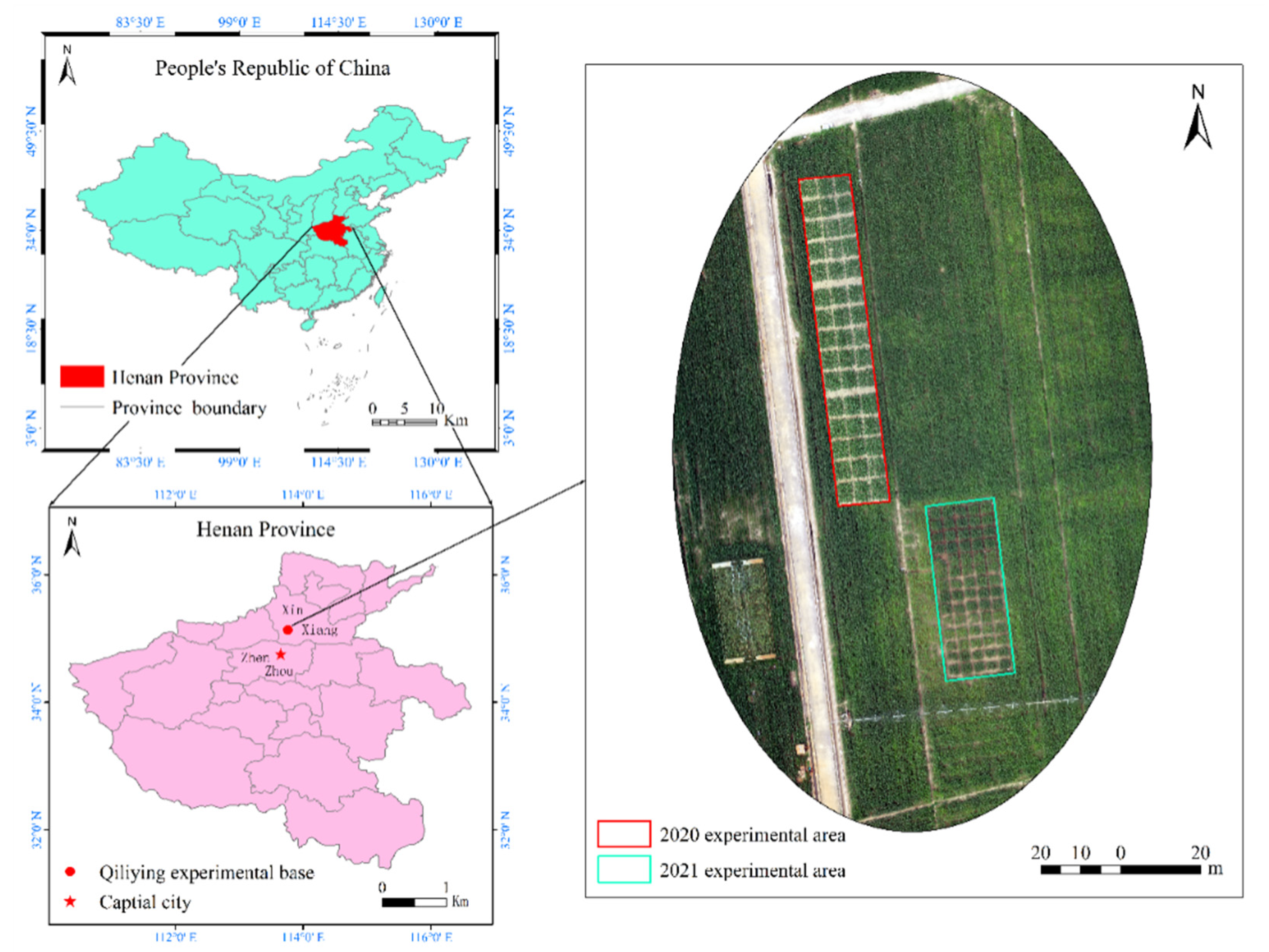
2.1. Overview of the Experimental Site

The study was conducted at Qiliying comprehensive experimental station (QCES) of the Chinese academy of agricultural sciences, Xinxiang city in Henan province of China (Figure 1). The station lies at 35°13′ North and 113°76′ East with an average altitude of 78 m above mean sea level. The average annual temperature of the experimental site is 14.1 °C and the mean relative humidity is approximately 68%. A minimum average temperature of 0.7 °C is recorded in January while a maximum average temperature of 27.1 °C is recorded in July. The site is characterized by a unimodal rainfall regime with an average annual rainfall of 548.3 mm. Normally, rains occur between July and September. The annual evaporation recorded is 1748.4 mm. Most of the agricultural activities are rainfed, with wheat and maize being the major food crops throughout the year. The major source of irrigation water is the groundwater. The study site is light loam soil. The surface soil’s bulk density within the study sites measured is 1.4 g/cm3. Adjacent plots were selected for the two-year experiment in order to ensure the consistency of soil nutrients when sowing in the same planting year.

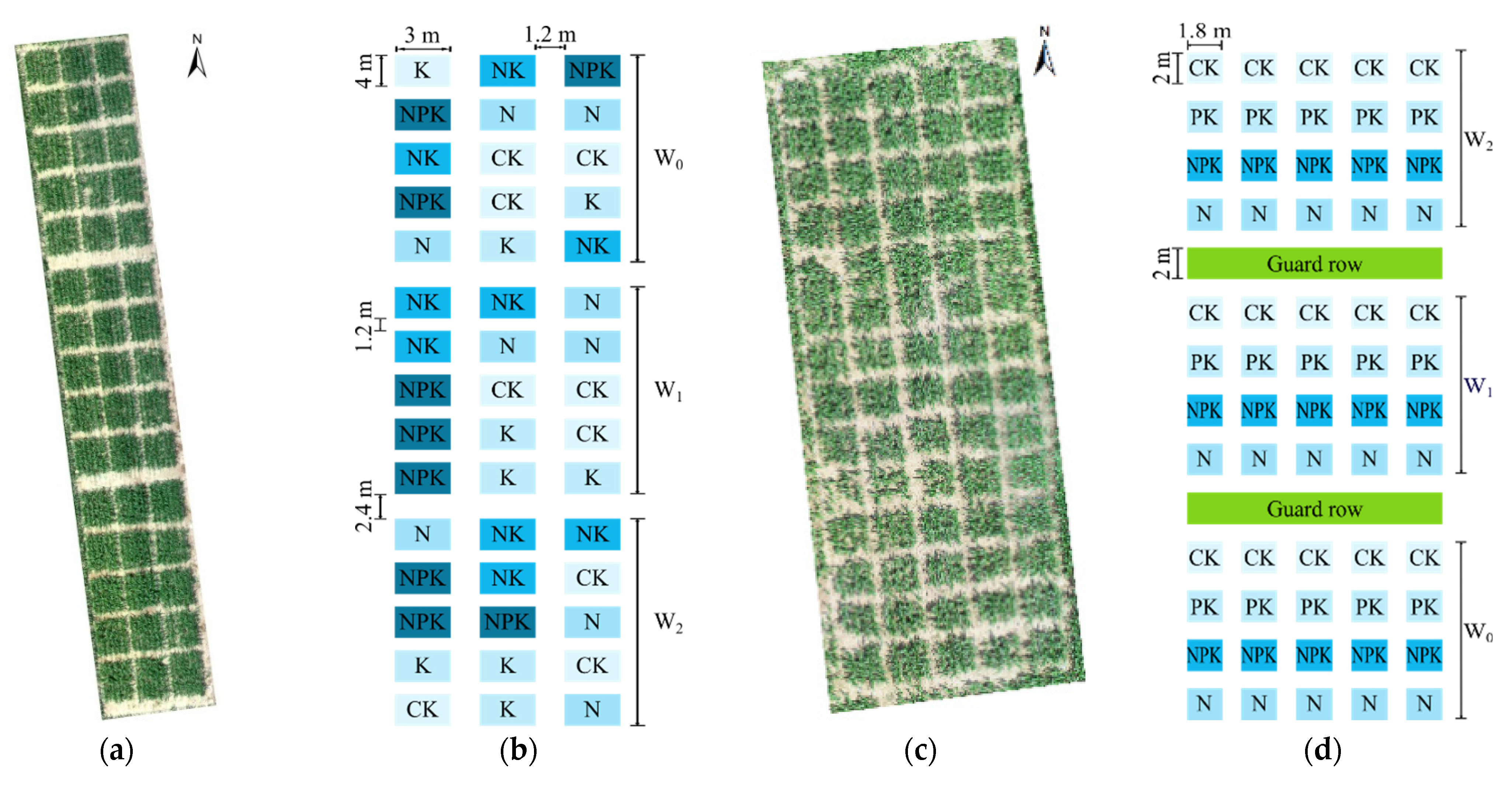
2.2. Experimental Design

Experimental fields were evaluated across two growing seasons, 2020 and 2021, for irrigation and fertilizer treatments (Figure 2). For this, two Maize cultivars “Taiyu 339” and “Nongda 108” were planted for two years on 20 June 2020 and 10 June 2021 with 0.6 m row spacing and 0.25 m plant spacing, and the row direction was North–South. The maize was headed on approximately 10 August and harvested on 27 September with a 96-day lifespan in 2020 and a 106-day lifespan in 2021.
In both years’ irrigation experiments, irrigation was carried out using the drip irrigation method with a total of three irrigation gradients. Irrigating quotas on each application were 0 mm (W0), 30 mm (W1) and 70 mm (W2), respectively. The irrigation volume was controlled by the water meter on the branch pipe. During the sowing period, the experimental field was irrigated with flood irrigation once, in order to ensure the emergence rate of maize. Afterwards, controlled irrigation treatments were carried out at the jointing stage, big trumpet stage and silking stage of summer maize.
In 2020, fertilizer treatments were conducted under each abovementioned irrigation treatment, using a completely randomized block design. Each irrigation treatment contained fifteen experiment plots of 4 × 3 m dimensions with 1.2 m spacing, with five fertilization treatments: CK, N, K, NK, NPK; where N, P, K are nitrogen (N, 250 kg hm−1), phosphate fertilizer (P2O5 30 kg hm−1) and potassium fertilizer (K2O 120 kg hm−1); CK is a non-nutritive fertilizer. Compound fertilizer (600 Kg hm−1) was basally applied to all plots, which accounted for 50% of the total application amount. Carbamide CO(NH2)2, superphosphate Ca(H2PO4)2·H2O, potassium chloride KCL were used as topdressing fertilizers. The topdressing time was at the big trumpet stage and silking stage; each application amount accounted for 25%. Five fertilizer treatments were repeated three times, as shown in Figure 2.
In 2021, the randomized block design was also used in the fertilization treatment experiment. However, each irrigation treatment contained twenty experiment plots (2 × 1.8 m) with 1.2 m spacing, with four fertilization treatments: CK, N, PK and NPK. Each fertilizer treatment was repeated five times. Fertilization application was divided into three times throughout the entire growth period, at the sowing stage, big trumpet stage and silking stage, while each application accounted for 33.3% of the total amount.

2.3. UAV Multispectral Images Acquisition and Process

UAV-based images were acquired using a RedEdge-MX (MicaSense, Inc., Seattle, WA, USA) sensor mounted on the DJI M210 (SZ DJI Technology Co., Shenzhen, China). The fields were georeferenced using UAV-mounted GPS. Then, the points were recorded to produce a flight route. The RedEdge-MX sensor had five multispectral bands (blue, green, red, red edge and near-infrared). The center wavelengths for the respective spectral band were 475 nm, 560 nm, 668 nm, 717 nm and 840 nm.
UAV flight missions were conducted under clear sky and low wind speed (<5 m s−1) conditions between 11:00 and 13:00 solar time, ensuring few shadows of features were collected. UAV acquired images of the field at a speed of 3 m s−1 and an altitude of 30 m above ground level. The 85% forward and 80% sideward overlap was set between images. A standard reluctance panel was used to calibrate the multispectral images.
Summer maize has a rapid growth from the jointing stage to silking stage and reached maximum LAI at the silking stage with no growth thereafter. Therefore, data collection was generally conducted from the jointing to silking stage as shown in Table 1.
UAV images were processed using the Pix4Dmaper 3.1.22 (Pix4D, S.A., Lausanne, Switzerland) to calibrate and stitch the acquired images. The software output included the experiment map, dense point cloud extraction and digital surface model (DSM). The point clouds were accurately georeferenced to the Earth reference system, World Geodetic System 84. The shape files were produced to clip each plot from the experimental map, then the average reflectivity of the plot in each band was respectively extracted to represent the actual reflectance of the plot. This part of the work was implemented in ArcGIS 10.5 (ESRI, RedLands, CA, USA). In the next step, ENVI 5.5 (Exelis Visual Information Solutions, Boulder, CO, USA) and IDL language were used to calculate the vegetation indices. The vegetation index can simply and effectively measure the growth of crops. It is widely used to estimate LAI [10]. In order to reduce the influence of external environmental factors, such as soil and atmosphere, 12 vegetation indices that perform well in this condition were selected according to previous studies [29]. The calculation formula of the 12 VIs is respectively shown in Table 2.

2.4. Ground Data Acquisition

The weather data was measured with 30 min intervals by the agricultural meteorological station installed on the flux tower near the experimental site. The parameters recorded include air temperature, relative humidity, wind speed, soil temperature and rainfall, etc. The ground truth LAI was measured by the SunScan (Delta-T Devices Ltd., Cambridge, UK) device. Each experiment plot was measured at one-third equal intervals along the planting direction, and the measurement direction was perpendicular to the planting direction; therefore, each experiment plot was completely measured three times, and the averaged LAI value of the plot was considered as the true LAI representative of the plot. The LAI measurement was performed after UAV image acquisition to ensure data synchronization.

2.5. Ensemble Learning Model Construction and Evaluation

The core idea of stacking in this study was to train the base model of the first layer, and then use the output of the first layer model as input to train the next-level model, to finally obtain the simulated value. In this study, only two layers of learners were set. At the same time, since each base model must be used as the input variable of the secondary learner, the selection of the primary model should follow some principles [39]. Firstly, the ensemble method combines the estimated values of a single model, and the performance of each primary model can affect the final ensemble result, so each primary model should have good estimation ability [40]. Secondly, there should be differences among the models.
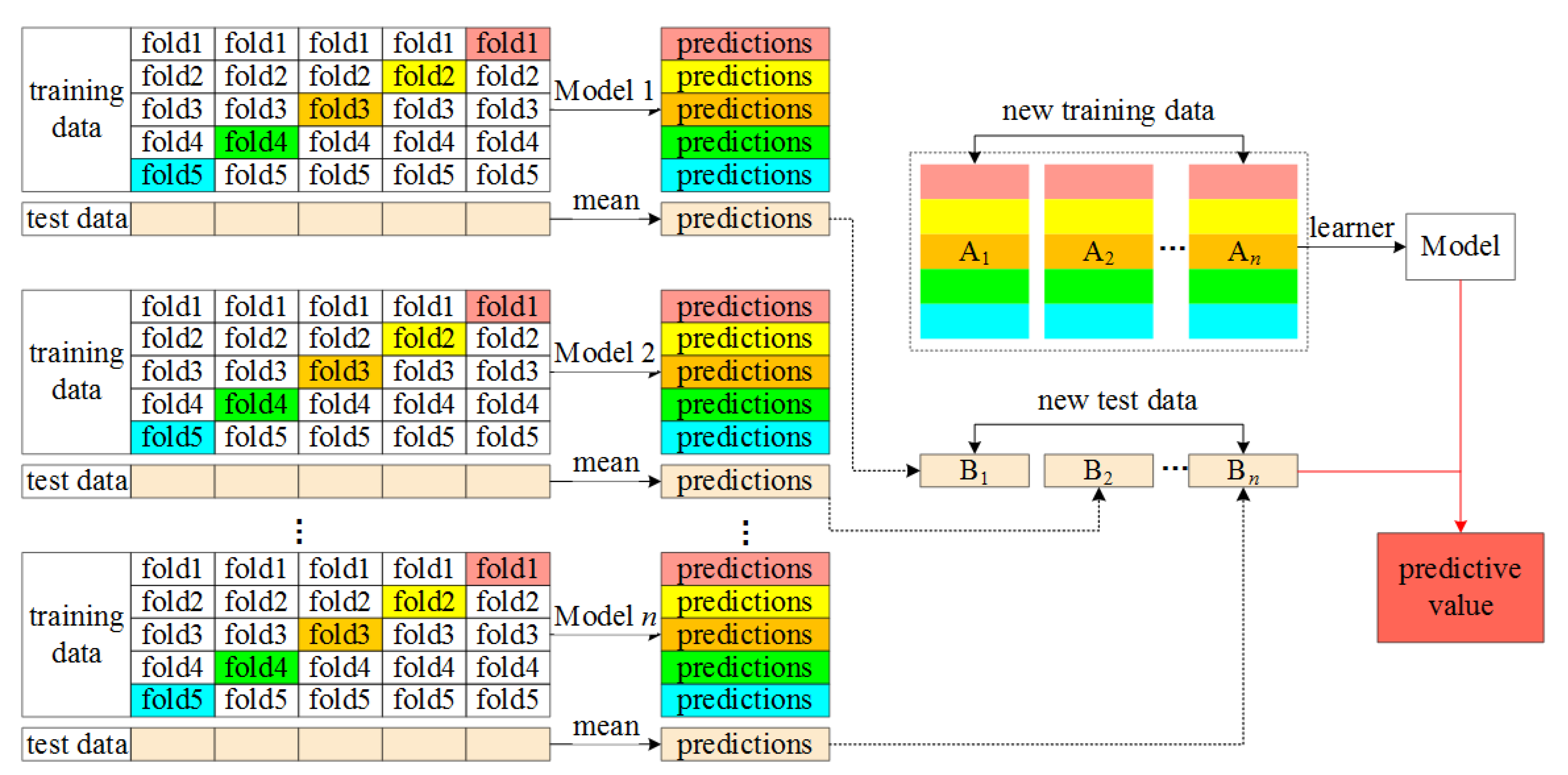
The basic principle of this algorithm is shown in Figure 3. Firstly, the data was divided into training set and test set, while the training set was divided into five parts: fold1, fold2, fold3, fold4 and fold5. Secondly, the primary learners (basic model) were selected, and the five-fold cross validation method was used for model training, and the trained basic model was used to predict the test set. Then, the predicted values of the training set were regarded as eigenvectors “A1, A2,…, An” to form a new training set; whereas, the predicted values of the test set were regarded as eigenvectors “B1, B2,…, Bn” to form a new test set. Finally, a predictive model was built using the secondary learner. In this study, primary learning models included Gaussian process regression (GPR), support vector regression (SVR), random forest (RF), least absolute shrinkage, selection operator (Lasso) and Cubist regression, while secondary learning models included RF and multiple linear regression (MLR). Model construction was performed using R 4.0.3. For more information, please refer to the literature [41,42].

2.5.1. Stepwise Regression

In order to obtain the high-performance model, the characteristic variables need to be screened prior. Stepwise regression is used to screen all parameters. Stepwise regression combines forward stepwise regression and backward stepwise regression. Only one variable is added each time, but in each step, the variable will be re-evaluated, and the variable with no or insignificant contribution to the current model can be removed. Independent variables can be added or removed again until an optimal model is obtained. Akaike information criterion (AIC) is used as the basis to judge whether the variable can survive [43]. The AIC formula is shown in Equation (1). Increasing the number of independent variables in the model can improve the goodness of fitting, but it may lead to over-fitting of the model. AIC encourages the goodness of data fitting and tries to avoid over-fitting. Therefore, the preferred model should be the one with the lowest AIC value. Using AIC to deal with statistical problems can be roughly divided into the following three steps: (1) constructing the statistical model; (2) the parameters are estimated by the maximum likelihood estimation method; (3) the model is selected by the minimization of AIC. The difference in AIC first depends on the likelihood function L. When there is no significant difference in L, the model with few parameters is considered to be a good model. Therefore, the model with better goodness of fit and few independent variables can be developed according to AIC.
AIC = - 2 ln L + 2 k
where k is the number of parameters; L is the likelihood function, which can be expressed as Equation (2):
L = n 2 ln 2 π n 2 ln SSE n n 2
where n is the sample size; SSE is the sum of squares error. It can be seen that L mainly depends on the sum of squares error. Therefore, AIC can also be expressed as Equation (3):
AIC = n   ln SSE n + 2 k

2.5.2. Gaussian Process Regression

Gaussian process regression (GPR) is a machine learning algorithm based on the Gaussian process (GP) for regression prediction of observed samples. The probability density function of the GP is shown in equation 4. It can be seen from the formula that the Gaussian distribution is determined by the mean vector and the covariance matrix. The process of GPR prediction can be roughly summarized into five steps: (1) determine the observed data points as the sampling points of the GP; (2) determine the mean function and covariance function; (3) obtain the function of the observed data according to the posterior probability expression; (4) use maximum likelihood estimation to solve hyperparameters; (5) get predicted values. The specific process can be followed in Rasmussen’s research [44].
p x 1 , x 2 , , x n = 1 2 π n 2 σ 1 σ 2 σ n exp 1 2 x 1 μ 1 2 σ 1 2 + x 2 μ 2 2 σ 2 2 + + x n μ n 2 σ n 2

2.5.3. Support Vector Regression

The support vector machine (SVM) is a classifier, but it can also be used for regression analysis. The application model of SVM regression is called support vector regression (SVR) [45]. The advantage of SVR is to determine the final decision function with a few support vectors. The complexity of its calculations depends on the support vector rather than the whole sample space, which can avoid the “disaster of dimension”. Similarly, the final result is determined by a few support vectors, which is not only convenient to pay attention to key samples, but also ensures that the SVM has good “robustness”. For nonlinear problems, the main idea of SVR is to transform the original problem into a linear problem in a high-dimensional space and perform a linear solution in the high-dimensional space. Then, the solution of the problem becomes maximizing the following objective function (Equation (5)) under the constraint condition (Equation (6)).
W α i , α i * = i = 1 n y i α i * α i ε i = 1 n α i + α i * 1 2 i = 1 n j = 1 n α i + α i * K x i , x j
i = 1 n α i + α i * = 0 0 α i , α i * C
where α i , α i * is Lagrange factor; W is objective function; ε and C are both positive constants; K x i , x j is kernel function. Finally, using the optimization algorithm to calculate equation 5 can be obtained by the nonlinear regression function (Equation (7)). In this formula, only a small part of α i * α i 0 , and their corresponding samples are called support vectors. The optimization algorithm can be expressed as Equation (8).
f x = α i * α i K x i , x j + b
min β   1 2 β T H β + γ T β
where β = α α * , H = X X T X X T X X T X X T , γ = ε + Y ε Y , X = x 1 x n , Y = y 1 y n . The constraint conditions of Equation (8) are β*(1, ∙∙∙, 1, −1, ∙∙∙, −1) = 0, and α i * , α i 0 and i = 1, ∙∙∙, n; n is sample size.

2.5.4. Cubist Regression

The Cubist model is an extension of the M5 model tree developed by Quinlan [46]. Cubist is a modeling analysis method based on specific rules, which is usually used in continuous value prediction problems. Firstly, the model tree is created through recursive processing and then simplified into a series of rules. These rules partition samples according to their spectra and a unique linear model is then applied to predict the target variable. The Cubist method can use the nearest neighbors in the sample to modify the model prediction results. The first step is to build a model tree. If there is a sample to be predicted, this method can find the closest one in the sample and finally get the predicted value. The independent variables in this method cannot only be used for modeling, but can also determine node branching. Using this algorithm in R, it is possible to automatically identify independent variables that can be used for branching and modeling. More details on Cubist and its implementation can be found in Viscarra Rossel and Webster and Minasny and McBratney [47,48].

2.5.5. Lasso Regression

Lasso regression is not only a model with good generalization and estimation ability, but also acts as a stable variable filter [49,50]. When the autocorrelation of variables is high, this kind of method can avoid excessive interpretation of the current sample and explore the law applicable to the whole population. This shift from explanation to prediction is helpful to enhance the theoretical significance and application value of research. The loss function of Lasso regression can be expressed as Equation (9). The first part of the formula is the loss function of ordinary least square (OLS), and the second part is the penalty function. λ (≥0) represents the tuning parameter, which is used to control the regression coefficient. The larger the value, the stronger the punishment. When λ = 0, it means that the regression model is not penalized, and the formula becomes the OLS loss function.
L Lasso β = | | Y X β | | 2 + λ W T β
where X is the matrix of predictive variables; Y is a vector of outcome variables; β is the regression coefficient vector; W is the vector with a value of ±1 (plus or minus sign corresponds to the corresponding value in the β vector).

2.5.6. Random Forest Regression

The random forest regression model consists of multiple decision trees, and there is no relationship between each decision tree in the forest. The final output of the model is jointly determined by each decision tree in the forest [51]. The randomness of random forest is reflected in two aspects: (1) A certain number of samples are randomly selected from the training set as the root node samples of each regression tree; (2) when establishing each regression tree, a certain number of candidate features are randomly selected, and the most suitable feature is selected as the split node.

2.5.7. Model Accuracy Evaluation

In this study, the coefficient of determination (R2), root mean square error (RMSE), residual prediction deviation (RPD) and the ratio of performance to interquartile distance (RPIQ) were used as the accuracy evaluation indexes. Among them, R2 can characterize the stability of the model (positive relationship) and RMSE is often used to characterize model accuracy (reverse relationship), while RPD is the ratio of sample standard deviation (SD) to RMSE (Equation (10)).
R P D = S D R M S E  
When 1.5 < RPD < 2.0, it is considered that the model can only roughly estimate the LAI; when 2.0 ≤ RPD < 3.0, the model has good prediction ability and is relatively reliable; when RPD ≥ 3.0, the model has excellent prediction ability and is reliable.
RPIQ considers both the prediction error and the change in observation data. It is a more objective and easier index to compare in model verification. The larger the RPIQ, the stronger the prediction ability of the model. Different from the residual prediction deviation, RPIQ has no assumption on the distribution of observed values [52]. Its formula is as shown in Equation (11):
R P I Q = I Q R M S E  
where IQ is the difference between the third and first quartiles.

3. Results

3.1. LAI under Different Water and Fertilizer Treatments

Before conducting analysis of variance (ANOVA), it is necessary to perform normal analysis on the data. If the data does not obey the normal distribution, the statistical conclusions obtained may be invalid. Thus, Figure 4 shows the normality test of experimental LAI data through Quantile-Quantile (Q-Q) image under the two treatments. It can be seen from the figure that the data was normally distributed across the stages.
Analysis of variance (ANOVA) results shows that the effect of irrigation and fertilization treatments on LAI. The F test and p-value in ANOVA results are important indicators to judge the significance of factors. The results in Table 3 and Table 4 indicate significantly effect of fertilizer and water stress on LAI.
Figure 5 shows the LAI development of summer maize in both years under different water and fertilizer treatments. Firstly, the LAI responded strongly to fertilizer treatment. The results, obtained from the two years of experiments, demonstrated that the average value of the maize LAI under NPK treatment is higher than that under CK treatment. Secondly, irrigation treatments also significantly influenced the LAI. With the increase in irrigation amount, the LAI gradually increased for each growing stage, especially in 2020. Thirdly, the combination of water and fertilizer further improved the maize LAI. In both years, under the W2 irrigation and NPK fertilization conditions, the average LAI at each stage were the highest. In addition, the highest average LAI value of each treatment was 4.422 in 2020 and was 2.820 in 2021. This big difference is due to the waterlogging inhibiting maize growth, resulting from heavy rainfall at big trumpet in 2021. Meanwhile, the waterlogging causes a decrease in the LAI after big trumpet in 2021. According to statistics, from 17–23 July to 2021, the cumulative rainfall in the experiment area was 512 mm, which was about to reach the average annual precipitation of 548.3 mm.

3.2. Correlation Analysis of Multispectral VIs and Ground LAI

Correlation between UAV-based vegetation indices (Vis) and the ground truth LAI were calculated at all growth stages using a simple linear regression model (Table 5). On the whole, the LAI showed significantly high (at p < 0.0001) correlations ranging from 0.573 to 0.890 with UAV-based VIs at each growth stage. Variation in the correlation values among the growth stages were due to the influence of spectral saturation, soil background and other factors, such as a single vegetation index, can have regional specificity and timeliness. The correlations were increased as the maize growth progresses. After the big trumpet stage, the correlation between the UAV-based Vis and the ground truth LAI were higher than at the jointing stage, due to the full stretch of leaves. From the jointing stage to the silking stage, the mean values of the coefficients of determination R2 for the LAI and UAV-based VIs were increased from 0.464 (In 2020) and 0.427 (In 2021) to 0.601 and 0.72, respectively. The main reason of increase is that the maize plants were short at the jointing stage, and the difference of ground coverage in the test area was low. Therefore, the probability of measurement errors was relatively high, resulting in a low correlation at the jointing stage.

3.3. Evaluation of Model Accuracy for LAI Prediction

Regression analysis has a strong dependence on the sample data. If the sample size is too small (≤60), the data sample distribution is insufficient, resulting in weak accuracy and robustness of the model for the single growth stage. Thus, data for all growth stages in same experiment were served as a new dataset to evaluate the robustness of the LAI estimation model. The new sample size was 180 in 2020 and 240 in 2021. In order to predict the relationship between ground truth LAI and UAV-based VIs in the new sample, univariate polynomial regression equation between LAI and UAV-based VIs was fitted. When the multi-growth stages were fused, the relationship between the LAI and VIs was not a simple first-order linear relationship. The fitting curves of the quadratic, cubic, and quartic polynomials performed well. Considering the simplicity of the model, quadratic polynomial was chosen to build the model. The univariate regression model and accuracy evaluation of the LAI and each of the VIs are shown in Table 6. It can be found that the ground truth LAI is significantly correlated with VIs, and the coefficient of determination R2 was greater than 0.87, the RMSE was lower than 0.38.
The number of parameters is another important factor affecting the performance of machine learning models. In the model hypothesis, some unconsidered factors are often regarded as random perturbation terms. The more explanatory variables mean the stronger relationship between parameters and random perturbation, which leads to the unbiased and inconsistent parameter estimation. Under-fitting and over-fitting should be avoided as far as possible for the regression model used for prediction. Therefore, filtering variables is an essential task when building a model. However, in our results, the correlation between the LAI and each VI was not significantly different. Therefore, the VIs need to be further screened by other methods.

3.4. Stepwise Selection of Feature Variables

The stepwise regression method based on the precise AIC criterion was used to screen the VIs. The stepwise regression analysis results are shown in Table 7. Compared with the previous univariate regression model, the accuracy of the multiple regression model has been improved. In the two years of results of stepwise regression equation, the performance of each VI was slightly different. For example, MSR did not perform well in the regression equation in 2020, while it contributed significantly to the model in 2021. Based on the performance of VIs in the two-year model, five Vis, i.e., GWDRVI, RESAVI, MSAVI2, NRI and NDRE, which have significant contributions for LAI estimation, were finally selected. In addition, NDVI is the most commonly used vegetation index. Considering the universality of the model, we artificially added NDVI to the five selected vegetation indices. Finally, there was a total of six independent variables used to build the ensemble learning model.

3.5. Performance Analysis of LAI Inversion Model

Based on the six selected VIs, GPR, SVR, Lasso, Cubist, MLR and RF regression algorithms were used to estimate the maize LAI. Table 8 shows the R2, RMSE, RPD and RPIQ values of the base model and secondary model for test set, to evaluate the estimation ability and stability of the model. The accuracy results of five primary learners for the test set showed that the SVR, Lasso and Cubist models were more robust in the two years than GPR and RF models, with higher R2, RPD, RPIQ and lower RMSE. The optimal evaluation parameters were produced by the SVR model with R2 = 0.965, RPD = 5.312, RPIQ = 8.213 and RMSE = 0.204 in 2020 and R2 = 0.897, RPD =3.135, RPIQ = 4.022 and RMSE = 0.221 in 2021. Figure 6 also shows more robust SVR, Lasso and Cubist models.
In order to integrate the estimation ability of five primary learners, two machine learning algorithms based on linear (MLR) and nonlinear (RF) models were selected as auxiliary learners. The results show that when MLR was used as the secondary learner, the model achieved the highest accuracy. The R2 values of the models are 0.967 and 0.897 for the two years, respectively. However, the accuracy in terms of R2 values did not improve significantly. Figure 6 shows the superior performance of the StMLR model. The violin shape of the StMLR model was better and more stable than other models. This result reflects the important role of the ensemble learning algorithm. Due to the differences of geographical crop location, growth environment and varieties, the model constructed by a single algorithm may not always get good estimation results. At this time, the integrated learning algorithm can synthesize the results of multiple base models to get the best output, ensuring the stability of the model. For example, when predicting the LAI of Maize in 2021, the RPD of GPR and RF base model (2.866, 2.871) was lower than 3.0, which was only moderately evaluated according to the standard. However, after learning through the MLR secondary learner, the RPD of the integrated model reached 3.142, which has excellent estimation ability and stability.
Figure 7 shows the distribution of the base model coefficients in the results of 400 iterations of the secondary model (MLR). The results show that among secondary learners, base models with higher accuracy were always given higher weights. This also reflects the working mechanism of the stacking algorithm. Instead of taking the output of the well-performing base model directly as the final output, the output result closest to the true value was obtained by combining the primary learners.
The best model of LAI achieved from the StMLR method was compared with corresponding observed values using scatterplots, as shown in Figure 8. It shows that the estimation effect of the model was excellent.

4. Discussion

The development of crop cultivation and management strategies for efficient use of resources to enhance crop stability and yield is very important. Therefore, continuous assessments of important traits such as LAI under different water and fertilizer conditions can help to understand their effect on crop growth and to develop different crop management strategies. In this study, we successfully evaluated the UAV-based multispectral phenotyping and stacking ensemble learning approach to estimate the LAI as an indicator for the assessment of water and fertilizer stress in summer maize. Previously, several studies have reported spectral information as a good predictor of phycological characteristics of the crops.
The relation between VIs and LAI is complex. In this study, the regression model with the lowest AIC value was selected by the stepwise regression method. Then the VI was selected according to the relative importance. Finally, five vegetation indexes with the best performance were selected to use as input for predictions. There is no doubt that more VIs with high correlation or with low correlation need to be compared before being used for LAI model generation. Meanwhile, other feature selection methods can be introduced to screen VIs more accurately, such as mRMR [53] and least angle regression (LARS) [54].
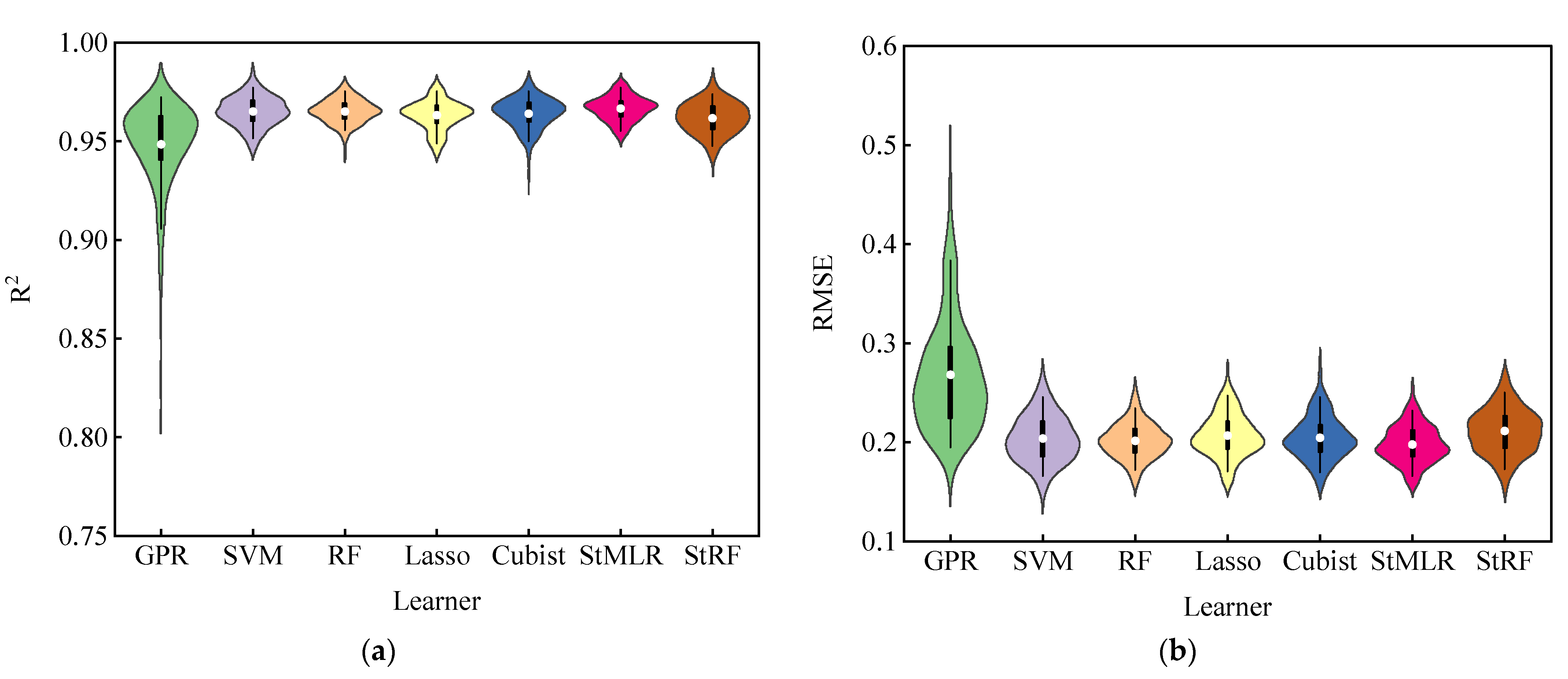
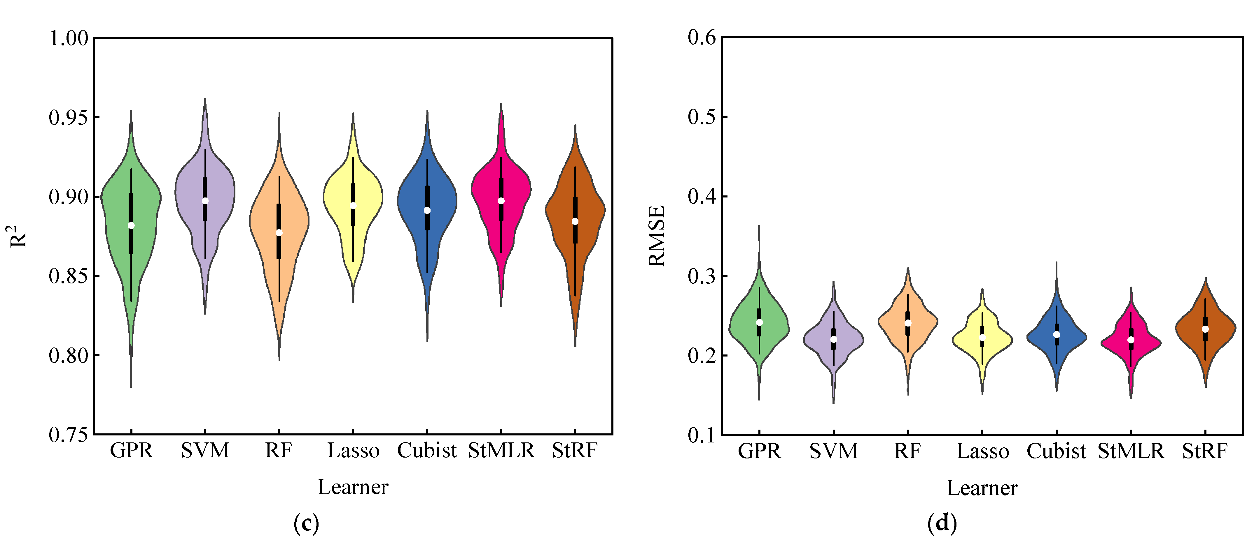
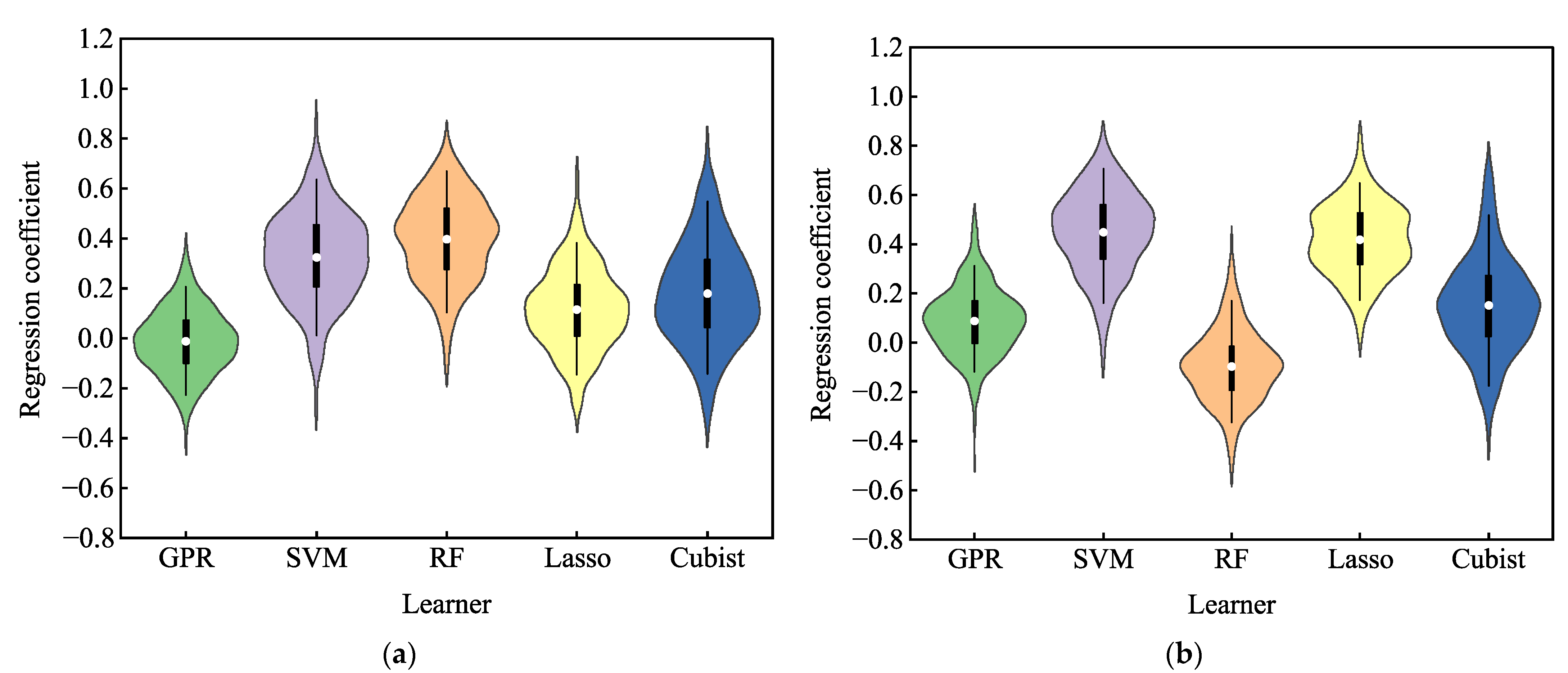
In this paper, five machine algorithms including GPR, SVM, RF, Lasso and Cubist were used as basic learners to build ensemble learning models using two years of data of maize LAI. The estimation ability of the five basic models was evaluated through four evaluation indicators. The results showed that among the models constructed by these five classical machine learning algorithms, the coefficient of determination (R2) between the output value and the real LAI was high, but the RPD of GPR and RF models were less than 3.0 when predicting maize LAI in 2021. These results indicated that the model constructed by using a single machine learning algorithm was unstable and there was a risk of error estimation [40]. Previously, Yuan et al. [55] found that the RF model was the most suitable for LAI estimation during the whole growth period. However, the RF as a basic model performed poorly in our results for the 2021 cropping season. The reasons for the inconsistent results from previous reports may be due to the use of different datasets and crops [56]. The RF basic model achieved better estimation results in the case of the 2020 dataset, which proves the correctness of the above analysis.
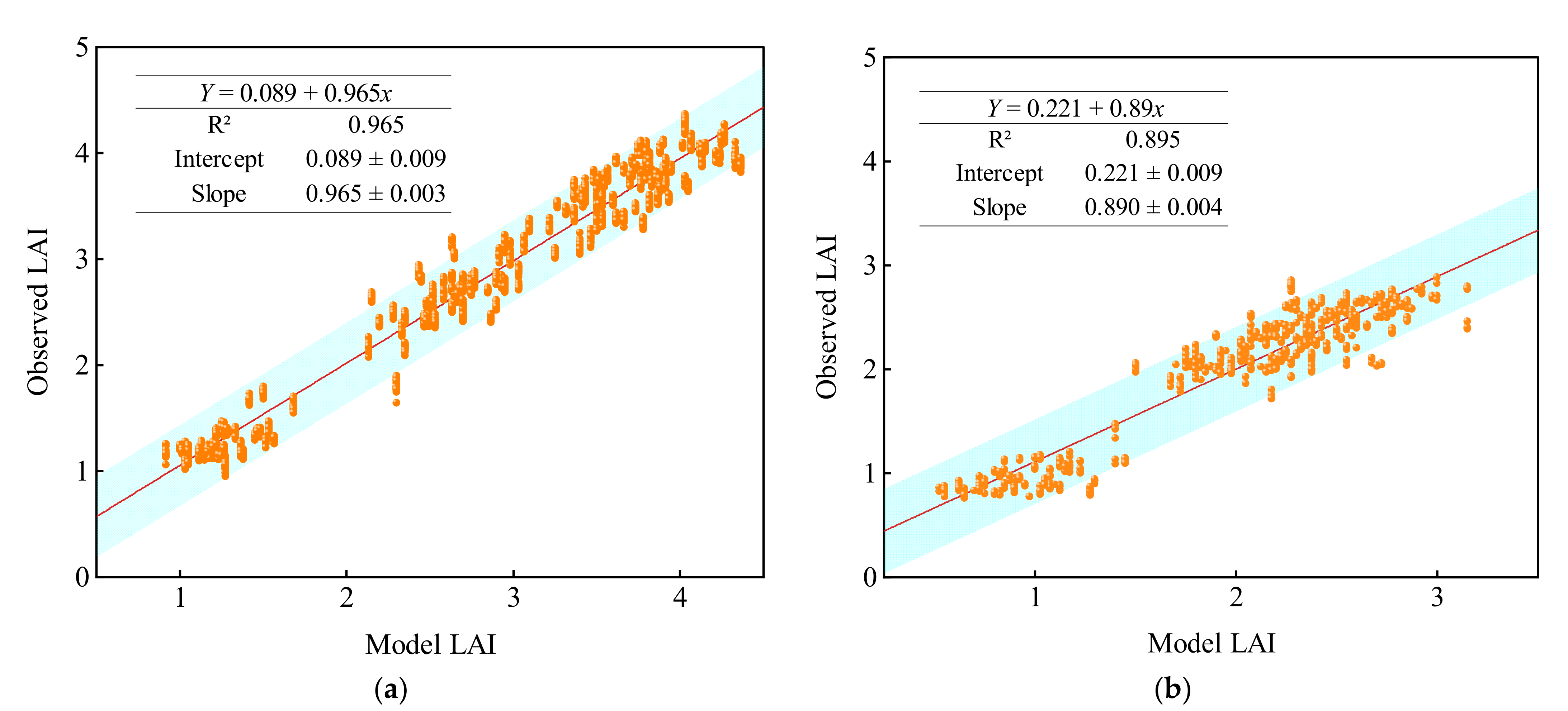
The performance of a single algorithm can be varied for different datasets, so it is difficult to optimize a single model-based estimation of traits under different modeling conditions. The ensemble learning algorithm can avoid the above phenomenon by stacking different base models. The stacking approach used in this study is an ensemble learning method, which has strong adaptability for different datasets. The anti-noise performance and fitting ability of the stacking algorithm has superiority over a single algorithm. The hypothesis space considered by different types of algorithms will also be different. If the real assumptions of some algorithms for the LAI of summer maize are not within the hypothesis space calculated by the currently selected model, then it is meaningless to use this algorithm for modeling. After integrating multiple regression algorithms through the stacking method, the corresponding hypothesis space will be expanded to a certain extent, thereby improving the universality of the model. In this study, the results state that the performance of the ensemble learning model was optimal in both years of data. Previously, some studies also demonstrated that the stacking method can improve the performance of the model in plant phenotype evaluation [57,58].
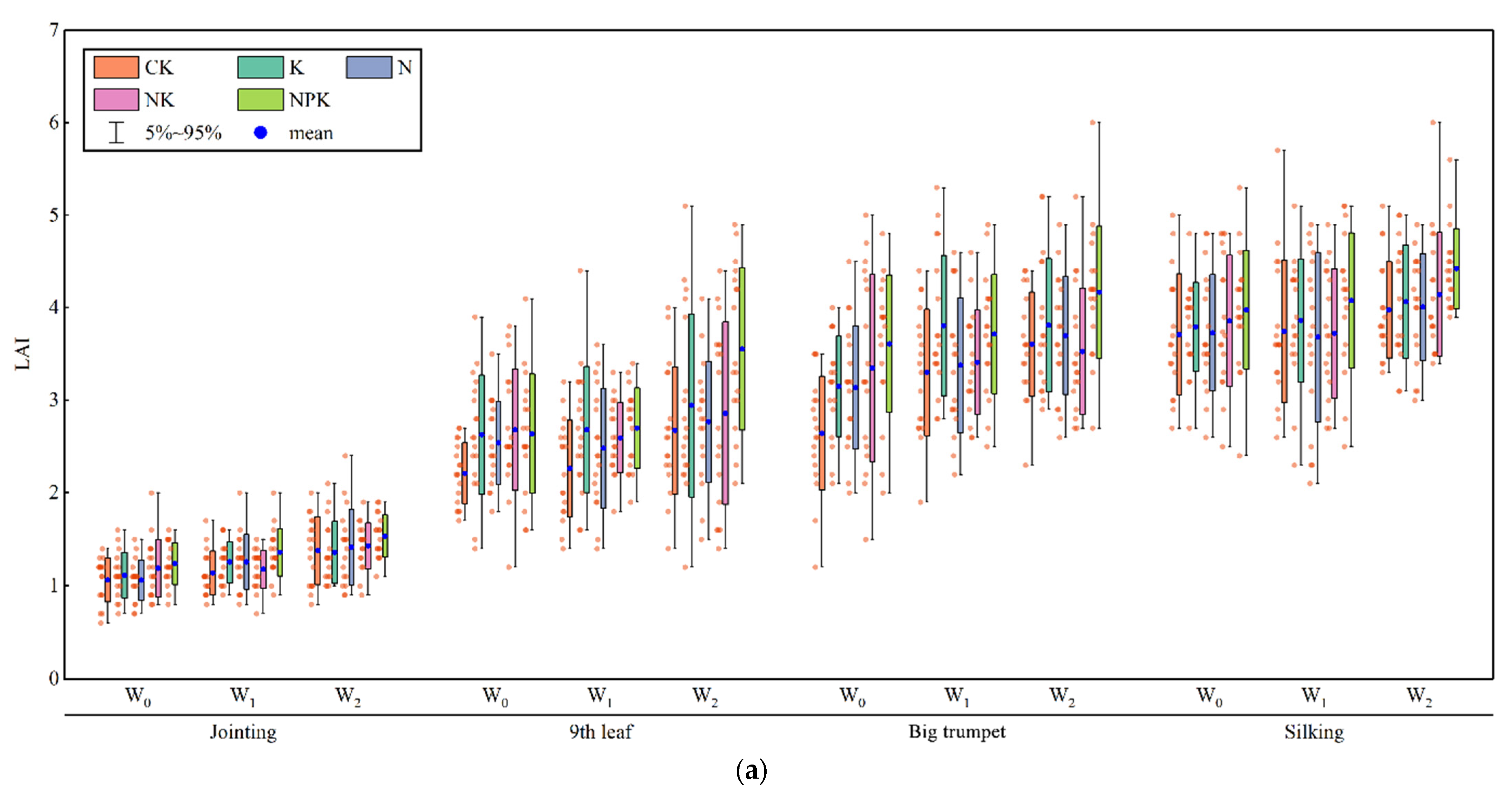
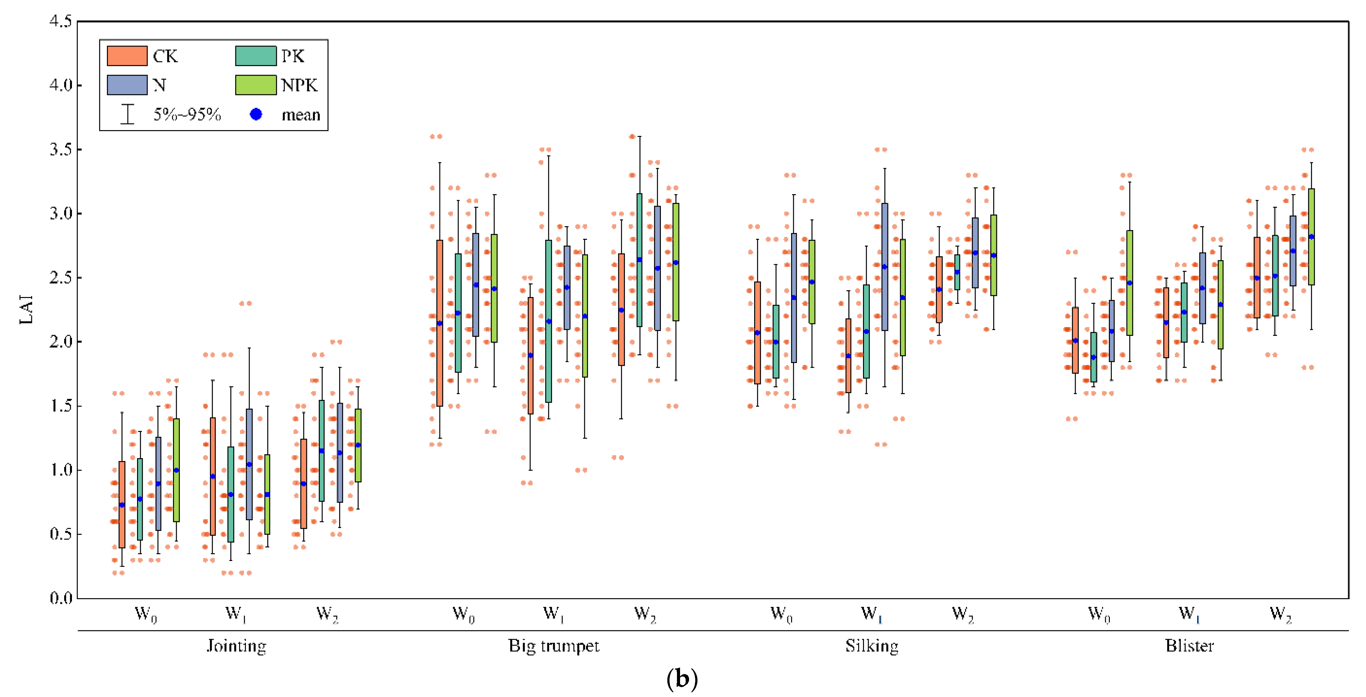
In this study, the irrigation method used for summer maize was drip irrigation and the amount of water per irrigation did not reach the field capacity. Therefore, there were different degrees of water stress under the three irrigation treatments W0 > W1 > W2. It was close to no deficit under W2 irrigation treatment conditions, which had little effect on the normal growth and development of summer maize. The water deficit was the most serious under the W0 irrigation treatment, which had a significant effect on the LAI over the whole growth period. At the same time, the LAI of the experimental plot with the most complete fertilizer ratio was better than that of the other fertilized plots, indicating that the LAI of summer maize can reflect the degree of fertilizer deficiency. More experiments with additional irrigation and fertilizer amount gradients should be set up to accurately diagnose the degree of irrigation and nutrient deficiency in each growth period of maize and realize intelligent and precise irrigation with integrated water and fertilizer.

5. Conclusions

This study discussed the changes in summer maize LAI under different water and fertilizer treatments and constructed a summer maize LAI estimation model using UAV-based phenotyping and machine learning ensemble algorithm. The main conclusions of this study are below:
(1)
We analyzed the relationship between different water and fertilizer treatments and LAI and found that LAI responded significantly to water and fertilizer stress in the two-year experiments. At the same time, the multispectral VIs were also significantly correlated with maize LAI at different growth stages. The Pearson correlation coefficient was not less than 0.639 and up to 0.89.
(2)
After the fusion of multiple growth periods, LAI and UAV-based VIs conformed to polynomial regression, and the correlation was significantly higher than that of a single growth period. The mean values of determination coefficient R2 between LAI and different vegetation indices reached 0.946 in 2020 and 0.887 in 2021.
(3)
The ensemble learning algorithm with MLR as the secondary learner outperformed from the single machine learning algorithm on the test set with R2 = 0.967, RMSE = 0.198 in 2020 and R2 = 0.897, RMSE = 0.220 in 2021. The RPD of the two-year model was greater than 3.0, indicating that the model was more stable.
These findings suggest that the LAI can characterize the effect of water and fertilizer stress in crops, while the ensemble learning algorithm can replace a single machine learning algorithm to build the LAI estimation model. This study provides some theoretical support for automated water and fertilizer management.

Author Contributions

Conceptualization, Q.C. and Z.C.; methodology, Q.C.; formal analysis, Q.C., H.X. and S.F.; data curation, H.X. and Z.L.; writing—original draft preparation, Q.C.; writing—review and editing, H.X., S.F., Z.L. and Z.C. All authors have read and agreed to the published version of the manuscript.

Funding

This research was funded by the Central Public-interest Scientific Institution Basal Research Fund (No. Y2021YJ07, FIRI2022-13 and FIRI2022-23).

Institutional Review Board Statement

Not applicable.

Informed Consent Statement

Not applicable.

Data Availability Statement

Not applicable.

Acknowledgments

The authors would like to thank the anonymous reviewers for their kind suggestions and constructive comments.

Conflicts of Interest

The authors declare no conflict of interest.

References

  1. Zhu, W.; Sun, Z.; Huang, Y.; Yang, T.; Li, J.; Zhu, K.; Zhang, J.; Yang, B.; Shao, C.; Peng, J.; et al. Optimization of Multi-Source UAV RS Agro-Monitoring Schemes Designed for Field-Scale Crop Phenotyping. Precis. Agric. 2021, 22, 1768–1802. [Google Scholar] [CrossRef]
  2. Gampe, D.; Zscheischler, J.; Reichstein, M.; O’Sullivan, M.; Smith, W.K.; Sitch, S.; Buermann, W. Increasing Impact of Warm Droughts on Northern Ecosystem Productivity over Recent Decades. Nat. Clim. Chang. 2021, 11, 772–779. [Google Scholar] [CrossRef]
  3. Victoria, G.; Jean-louis, D.; François, G. Review Article Water Deficit and Nitrogen Nutrition of Crops. A Review. Agron. Sustain. Dev. 2010, 30, 529–544. [Google Scholar]
  4. Aboelghar, M.; Arafat, S.; Abo Yousef, M.; El-Shirbeny, M.; Naeem, S.; Massoud, A.; Saleh, N. Using SPOT Data and Leaf Area Index for Rice Yield Estimation in Egyptian Nile Delta. Egypt. J. Remote Sens. Sp. Sci. 2011, 14, 81–89. [Google Scholar] [CrossRef] [Green Version]
  5. Irmak, S.; Mohammed, A.T.; Kukal, M.S. Maize Response to Coupled Irrigation and Nitrogen Fertilization under Center Pivot, Subsurface Drip and Surface (Furrow) Irrigation: Growth, Development and Productivity. Agric. Water Manag. 2022, 263, 107457. [Google Scholar] [CrossRef]
  6. Jiang, J.; Johansen, K.; Stanschewski, C.S.; Wellman, G.; Mousa, M.A.A.; Fiene, G.M.; Asiry, K.A.; Tester, M.; McCabe, M.F. Phenotyping a Diversity Panel of Quinoa Using UAV-Retrieved Leaf Area Index, SPAD-Based Chlorophyll and a Random Forest Approach. Precis. Agric. 2022, 23, 961–983. [Google Scholar] [CrossRef]
  7. Qiao, B.; He, X.; Liu, Y.; Zhang, H.; Zhang, L.; Liu, L.; Reineke, A.-J.; Liu, W.; Müller, J. Maize Characteristics Estimation and Classification by Spectral Data under Two Soil Phosphorus Levels. Remote Sens. 2022, 14, 493. [Google Scholar] [CrossRef]
  8. Homolová, L.; Malenovský, Z.; Clevers, J.G.P.W.; García-Santos, G.; Schaepman, M.E. Review of Optical-Based Remote Sensing for Plant Trait Mapping. Ecol. Complex. 2013, 15, 1–16. [Google Scholar] [CrossRef] [Green Version]
  9. Wang, X.; Zhang, R.; Song, W.; Han, L.; Liu, X.; Sun, X.; Luo, M.; Chen, K.; Zhang, Y.; Yang, H.; et al. Dynamic Plant Height QTL Revealed in Maize through Remote Sensing Phenotyping Using a High-Throughput Unmanned Aerial Vehicle (UAV). Sci. Rep. 2019, 9, 3458. [Google Scholar] [CrossRef] [Green Version]
  10. Xu, J.; Quackenbush, L.J.; Volk, T.A.; Im, J. Forest and Crop Leaf Area Index Estimation Using Remote Sensing: Research Trends and Future Directions. Remote Sens. 2020, 12, 2934. [Google Scholar] [CrossRef]
  11. Zhang, D.; Liu, J.; Ni, W.; Sun, G.; Zhang, Z.; Liu, Q.; Wang, Q. Estimation of Forest Leaf Area Index Using Height and Canopy Cover Information Extracted from Unmanned Aerial Vehicle Stereo Imagery. IEEE J. Sel. Top. Appl. Earth Obs. Remote Sens. 2019, 12, 471–481. [Google Scholar] [CrossRef]
  12. Cheng, Z.; Meng, J.; Shang, J.; Liu, J.; Huang, J.; Qiao, Y.; Qian, B.; Jing, Q.; Dong, T.; Yu, L. Generating Time-Series LAI Estimates of Maize Using Combined Methods Based on Multispectral UAV Observations and WOFOST Model. Sensors (Switzerland) 2020, 20, 6006. [Google Scholar] [CrossRef]
  13. Zhang, J.; Cheng, T.; Guo, W.; Xu, X.; Qiao, H.; Xie, Y.; Ma, X. Leaf Area Index Estimation Model for UAV Image Hyperspectral Data Based on Wavelength Variable Selection and Machine Learning Methods. Plant Methods 2021, 17, 49. [Google Scholar] [CrossRef] [PubMed]
  14. Li, Z.; Jin, X.; Wang, J.; Yang, G.; Nie, C.; Xu, X.; Feng, H. Estimating Winter Wheat (Triticum Aestivum) LAI and Leaf Chlorophyll Content from Canopy Reflectance Data by Integrating Agronomic Prior Knowledge with the PROSAIL Model. Int. J. Remote Sens. 2015, 36, 2634–2653. [Google Scholar] [CrossRef]
  15. Gong, Y.; Yang, K.; Lin, Z.; Fang, S.; Wu, X.; Zhu, R.; Peng, Y. Remote Estimation of Leaf Area Index (LAI) with Unmanned Aerial Vehicle (UAV) Imaging for Different Rice Cultivars throughout the Entire Growing Season. Plant Methods 2021, 17, 88. [Google Scholar] [CrossRef]
  16. Liu, S.; Jin, X.; Nie, C.; Wang, S.; Yu, X.; Cheng, M.; Shao, M.; Wang, Z.; Tuohuti, N.; Bai, Y.; et al. Estimating Leaf Area Index Using Unmanned Aerial Vehicle Data: Shallow vs. Deep Machine Learning Algorithms. Plant Physiol. 2021, 187, 1551–1576. [Google Scholar] [CrossRef]
  17. Chandrashekar, G.; Sahin, F. A Survey on Feature Selection Methods. Comput. Electr. Eng. 2014, 40, 16–28. [Google Scholar] [CrossRef]
  18. Rong, M.; Gong, D.; Gao, X. Feature Selection and Its Use in Big Data: Challenges, Methods, and Trends. IEEE Access 2019, 7, 19709–19725. [Google Scholar] [CrossRef]
  19. Cai, Y.; Guan, K.; Lobell, D.; Potgieter, A.B.; Wang, S.; Peng, J.; Xu, T.; Asseng, S.; Zhang, Y.; You, L.; et al. Integrating Satellite and Climate Data to Predict Wheat Yield in Australia Using Machine Learning Approaches. Agric. For. Meteorol. 2019, 274, 144–159. [Google Scholar] [CrossRef]
  20. Maimaitijiang, M.; Sagan, V.; Sidike, P.; Daloye, A.M.; Erkbol, H.; Fritschi, F.B. Crop Monitoring Using Satellite/UAV Data Fusion and Machine Learning. Remote Sens. 2020, 12, 1357. [Google Scholar] [CrossRef]
  21. Tian, Y.; Huang, H.; Zhou, G.; Zhang, Q.; Tao, J.; Zhang, Y.; Lin, J. Aboveground Mangrove Biomass Estimation in Beibu Gulf Using Machine Learning and UAV Remote Sensing. Sci. Total Environ. 2021, 781, 146816. [Google Scholar] [CrossRef]
  22. Wang, J.; Zhou, Q.; Shang, J.; Liu, C.; Zhuang, T.; Ding, J.; Xian, Y.; Zhao, L.; Wang, W.; Zhou, G.; et al. UAV-and Machine Learning-Based Retrieval of Wheat SPAD Values at the Overwintering Stage for Variety Screening. Remote Sens. 2021, 13, 5166. [Google Scholar] [CrossRef]
  23. Chatzimparmpas, A.; Martins, R.M.; Kucher, K.; Kerren, A. StackGenVis: Alignment of Data, Algorithms, and Models for Stacking Ensemble Learning Using Performance Metrics. IEEE Trans. Vis. Comput. Graph. 2021, 27, 1547–1557. [Google Scholar] [CrossRef]
  24. Li, Z.; Chen, Z.; Cheng, Q.; Duan, F.; Sui, R.; Huang, X.; Xu, H. UAV-Based Hyperspectral and Ensemble Machine Learning for Predicting Yield in Winter Wheat. Agronomy 2022, 12, 202. [Google Scholar] [CrossRef]
  25. Razavi-Termeh, S.V.; Sadeghi-Niaraki, A.; Choi, S.M. Spatial Modeling of Asthma-prone Areas Using Remote Sensing and Ensemble Machine Learning Algorithms. Remote Sens. 2021, 13, 3222. [Google Scholar] [CrossRef]
  26. Ustuner, M.; Sanli, F.B. Polarimetric Target Decompositions and Light Gradient Boosting Machine for Crop Classification: A Comparative Evaluation. ISPRS Int. J. Geo-Inf. 2019, 8. [Google Scholar] [CrossRef] [Green Version]
  27. Ge, H.; Ma, F.; Li, Z.; Tan, Z.; Du, C. Improved Accuracy of Phenological Detection in Rice Breeding by Using Ensemble Models of Machine Learning Based on Uav-rgb Imagery. Remote Sens. 2021, 13, 2678. [Google Scholar] [CrossRef]
  28. Ilniyaz, O.; Kurban, A.; Du, Q. Leaf Area Index Estimation of Pergola-Trained Vineyards in Arid Regions Based on UAV RGB and Multispectral Data Using Machine Learning Methods. Remote Sens. 2022, 14, 415. [Google Scholar] [CrossRef]
  29. Haboudane, D.; Miller, J.R.; Pattey, E.; Zarco-Tejada, P.J.; Strachan, I.B. Hyperspectral Vegetation Indices and Novel Algorithms for Predicting Green LAI of Crop Canopies: Modeling and Validation in the Context of Precision Agriculture. Remote Sens. Environ. 2004, 90, 337–352. [Google Scholar] [CrossRef]
  30. Xue, J.; Su, B. Significant Remote Sensing Vegetation Indices: A Review of Developments and Applications. J. Sensors 2017, 2017, 1353691. [Google Scholar] [CrossRef] [Green Version]
  31. Chen, J.M. Evaluation of Vegetation Indices and a Modified Simple Ratio for Boreal Applications. Can. J. Remote Sens. 1996, 22, 229–242. [Google Scholar] [CrossRef]
  32. Goel, N.S.; Qin, W. Influences of Canopy Architecture on Relationships between Various Vegetation Indices and LAI and FPAR: A Computer Simulation. Remote Sens. Rev. 1994, 10, 309–347. [Google Scholar] [CrossRef]
  33. Zha, H.; Miao, Y.; Wang, T.; Li, Y.; Zhang, J.; Sun, W.; Feng, Z.; Kusnierek, K. Improving Unmanned Aerial Vehicle Remote Sensing-Based Rice Nitrogen Nutrition Index Prediction with Machine Learning. Remote Sens. 2020, 12, 215. [Google Scholar] [CrossRef] [Green Version]
  34. Tucker, C.J. Red and Photographic Infrared Linear Combinations for Monitoring Vegetation. Remote Sens. Environ. 1979, 8, 127–150. [Google Scholar] [CrossRef] [Green Version]
  35. Sripada, R.P.; Heiniger, R.W.; White, J.G.; Weisz, R. Aerial Color Infrared Photography for Determining Late-Season Nitrogen Requirements in Corn. Agron. J. 2005, 97, 1443–1451. [Google Scholar] [CrossRef]
  36. Cao, Q.; Miao, Y.; Wang, H.; Huang, S.; Cheng, S.; Khosla, R.; Jiang, R. Non-Destructive Estimation of Rice Plant Nitrogen Status with Crop Circle Multispectral Active Canopy Sensor. F. Crop. Res. 2013, 154, 133–144. [Google Scholar] [CrossRef]
  37. Lu, J.; Miao, Y.; Shi, W.; Li, J.; Yuan, F. Evaluating Different Approaches to Non-Destructive Nitrogen Status Diagnosis of Rice Using Portable RapidSCAN Active Canopy Sensor. Sci. Rep. 2017, 7, 14073. [Google Scholar] [CrossRef]
  38. Jiang, Z. Interpretation of the Modified Soil-Adjusted Vegetation Index Isolines in Red-NIR Reflectance Space. J. Appl. Remote Sens. 2007, 1, 013503. [Google Scholar] [CrossRef] [Green Version]
  39. Frame, J.; Merrilees, D.W. The Effect of Tractor Wheel Passes on Herbage Production from Diploid and Tetraploid Ryegrass Swards. Grass Forage Sci. 1996, 51, 13–20. [Google Scholar] [CrossRef]
  40. Feng, L.; Zhang, Z.; Ma, Y.; Du, Q.; Williams, P.; Drewry, J.; Luck, B. Alfalfa Yield Prediction Using UAV-Based Hyperspectral Imagery and Ensemble Learning. Remote Sens. 2020, 12, 2028. [Google Scholar] [CrossRef]
  41. Kuter, S. Completing the Machine Learning Saga in Fractional Snow Cover Estimation from MODIS Terra Reflectance Data: Random Forests versus Support Vector Regression. Remote Sens. Environ. 2021, 255, 112294. [Google Scholar] [CrossRef]
  42. Shao, G.; Han, W.; Zhang, H.; Liu, S.; Wang, Y.; Zhang, L.; Cui, X. Mapping Maize Crop Coefficient Kc Using Random Forest Algorithm Based on Leaf Area Index and UAV-Based Multispectral Vegetation Indices. Agric. Water Manag. 2021, 252, 106906. [Google Scholar] [CrossRef]
  43. Akaike, H. A New Look at the Statistical Model Identification. IEEE Trans. Automat. Contr. 1974, 19, 716–723. [Google Scholar] [CrossRef]
  44. Rasmussen, C.E. Gaussian Processes in Machine Learning. In Advanced Lectures on Machine Learning; Springer: Berlin/Heidelberg, Germany, 2003; Volume 3176, pp. 63–71. [Google Scholar]
  45. Klopfenstein, Q.; Vaiter, S. Linear Support Vector Regression with Linear Constraints. Mach. Learn. 2021, 110, 1939–1974. [Google Scholar] [CrossRef]
  46. Quinlan, J.R. Improved Use of Continuous Attributes in C4.5. J. Artif. Intell. Res. 1996, 4, 77–90. [Google Scholar] [CrossRef] [Green Version]
  47. Houborg, R.; McCabe, M.F. A Hybrid Training Approach for Leaf Area Index Estimation via Cubist and Random Forests Machine-Learning. ISPRS J. Photogramm. Remote Sens. 2018, 135, 173–188. [Google Scholar] [CrossRef]
  48. Northup, B.K.; Daniel, J.A. Near Infrared Reflectance-Based Tools for Predicting Soil Chemical Properties of Oklahoma Grazinglands. Agron. J. 2012, 104, 1122–1129. [Google Scholar] [CrossRef]
  49. Zou, H. The Adaptive Lasso and Its Oracle Properties. J. Am. Stat. Assoc. 2006, 101, 1418–1429. [Google Scholar] [CrossRef] [Green Version]
  50. Zou, H.; Hastie, T. Regularization and Variable Selection via the Elastic Net. J. R. Stat. Soc. Ser. B Stat. Methodol. 2005, 67, 301–320. [Google Scholar] [CrossRef] [Green Version]
  51. Breiman, L. Random Forests. Mach. Learn. 2001, 45, 5–32. [Google Scholar] [CrossRef] [Green Version]
  52. Guo, L.; Zhang, H.; Shi, T.; Chen, Y.; Jiang, Q.; Linderman, M. Prediction of Soil Organic Carbon Stock by Laboratory Spectral Data and Airborne Hyperspectral Images. Geoderma 2019, 337, 32–41. [Google Scholar] [CrossRef]
  53. Peng, H.; Long, F.; Ding, C. Feature Selection Based on Mutual Information: Criteria of Max-Dependency, Max-Relevance, and Min-Redundancy. IEEE Trans. Pattern Anal. Mach. Intell. 2005, 27, 1226–1238. [Google Scholar] [CrossRef]
  54. Efron, B.; Hastie, T.; Johnstone, I.; Tibshirani, R. Least Angle Regression. Ann. Stat. 2004, 32, 440–444. [Google Scholar] [CrossRef] [Green Version]
  55. Yuan, H.; Yang, G.; Li, C.; Wang, Y.; Liu, J.; Yu, H.; Feng, H.; Xu, B.; Zhao, X.; Yang, X. Retrieving Soybean Leaf Area Index from Unmanned Aerial Vehicle Hyperspectral Remote Sensing: Analysis of RF, ANN, and SVM Regression Models. Remote Sens. 2017, 9, 309. [Google Scholar] [CrossRef] [Green Version]
  56. Herrmann, I.; Pimstein, A.; Karnieli, A.; Cohen, Y.; Alchanatis, V.; Bonfil, D.J. LAI Assessment of Wheat and Potato Crops by VENμS and Sentinel-2 Bands. Remote Sens. Environ. 2011, 115, 2141–2151. [Google Scholar] [CrossRef]
  57. Fei, S.; Hassan, M.A.; Ma, Y.; Shu, M.; Cheng, Q.; Li, Z.; Chen, Z.; Xiao, Y. Entropy Weight Ensemble Framework for Yield Prediction of Winter Wheat under Different Water Stress Treatments Using Unmanned Aerial Vehicle-Based Multispectral and Thermal Data. Front. Plant Sci. 2021, 12, 730181. [Google Scholar] [CrossRef] [PubMed]
  58. Sun, W.; Trevor, B. A Stacking Ensemble Learning Framework for Annual River Ice Breakup Dates. J. Hydrol. 2018, 561, 636–650. [Google Scholar] [CrossRef]
Figure 1. Geographic location of the study area.
Agriculture 12 01267 g001
Figure 2. Distribution of the experimental plots. (a) Overview of experimental field in 2020; (b) Fertilization and irrigation treatments in 2020; (c) Overview of experimental field in 2021; (d) Fertilization and irrigation treatments in 2021.
Agriculture 12 01267 g002
Figure 3. Schematic diagram of stacking algorithm workflow.
Agriculture 12 01267 g003
Figure 4. Q-Q results of experimental data. (a) Jointing, 2020; (b) 9th leaf, 2020; (c) Big trumpet, 2020; (d) Silking, 2020; (e) Jointing, 2021; (f) Big trumpet, 2021; (g) Silking, 2021; (h) Blister, 2021.
Agriculture 12 01267 g004
Figure 5. LAI under different water and fertilizer treatments in (a) 2020 and (b) 2021.
Agriculture 12 01267 g005aAgriculture 12 01267 g005b
Figure 6. Statistical distribution of the LAI estimation accuracies for all levels of learners during the testing phase. (a) Model R2 in 2020; (b) Model RMSE in 2020; (c) Model R2 in 2021; (d) Model RMSE in 2021.
Agriculture 12 01267 g006aAgriculture 12 01267 g006b
Figure 7. Base model coefficient distribution in secondary models (MLR) in (a) 2020 and (b) 2021.
Agriculture 12 01267 g007
Figure 8. Estimation results of maize LAI by secondary models (MLR) in (a) 2020 and (b) 2021.
Agriculture 12 01267 g008
Table 1. Data acquisition dates.
20202021
UAV Flight DateField Sampling DateGrowth PeriodUAV Flight DateField Sampling DateGrowth Period
July 13July 13jointingJuly 12July 12jointing
July 24July 249th leafJuly 30July 30big trumpet
July 30July 30big trumpetAugust 11August 11silking
August 10August 10silkingAugust 19August 19blister
Table 2. Details of multispectral vegetation index.
Vegetation IndexFormulaReference
Normalized Difference Vegetation Index (NDVI) ( ρ N I R ρ R ) / ( ρ N I R + ρ R ) (Xue and Su, [30])
Modified Simple Ratio (MSR) ρ N I R / ρ R 1 / ( ρ N I R / ρ R + 1 ) (Chen, [31])
Nonlinear Index (NLI) ρ N I R 2 ρ R / ρ N I R 2 + ρ R (Goel and Qin, [32])
Modified Double Difference Index (MDD) ( ρ N I R ρ R E ) ( ρ R E ρ G ) (Zha et al., [33])
Difference Vegetation Index (DVI) ρ N I R ρ R (Tucker, [34])
Green Ratio Vegetation Index (GRVI) ρ N I R / ρ G (Sripada et al., [35])
Green Wide Dynamic Range Vegetation Index (GWDRVI) 0.12 ρ N I R ρ G / 0.12 ρ N I R + ρ G (Cao et al., [36])
Normalized Red Index (NRI) ρ R / ( ρ N I R + ρ R E + ρ R ) (Lu et al., [37])
Modified Normalized Difference Index (MNDI) ( ρ N I R ρ R E ) / ( ρ N I R ρ G ) (Lu et al., [37])
Normalized Difference Red Edge (NDRE) ( ρ N I R ρ R E ) / ( ρ N I R + ρ R E ) (Zha et al., [33])
Red Edge Soil-Adjusted Vegetation Index (RESAVI) 1.5 ( ρ N I R ρ R E ) / ( ρ N I R + ρ R E + 0.5 ) (Cao et al., [36])
Modified Soil-adjusted Vegetation Index ( MSAVI 2 ) 0 . 5 2 ρ N I R + 1 - ( 2 ρ N I R + 1 ) 2 -   8 ρ N I R - ρ N I R (Jiang et al., [38])
Note: G, NIR, R, RE are the averaged reflectance among the waveband range to match multispectral data in the green, near infrared, red, and red edge wavelengths, respectively.
Table 3. ANOVA results between LAI and control variables in 2020.
Control VariableJointing9th LeafBig TrumpetSilking
Fp-ValueFp-ValueFp-ValueFp-Value
Fertilization3.4280.0199.7973.418 × 10−58.2961.248 × 10−44.6740.005
Irrigation25.2663.69 × 10−720.7132.233 × 10−620.5632.379 × 10−612.0591.434 × 10−4
Note: the F-crit of fertilization factor is 2.69 (α < 0.05) and that of irrigation factor is 3.32.
Table 4. ANOVA results between LAI and control variables in 2021.
Control VariableJointingBig TrumpetSilkingBlister
Fp-ValueFp-ValueFp-ValueFp-Value
Fertilization2.6320.0616.8256.360 × 10−411.3899.277 × 10−65.8920.002
Irrigation9.5083.324 × 10−410.1552.100 × 10−415.0448.466 × 10−624.6944.224 × 10−8
Note: the F-crit of fertilization factor is 2.84 (α < 0.05) and that of irrigation factor is 3.23.
Table 5. Correlation between UAV-based vegetation indices and ground truth LAI.
Vegetation Index20202021
Jointing9th LeafBig TrumpetSilkingJointingBig TrumpetSilkingBlister
NDVI0.693 ***0.763 ***0.824 ***0.779 ***0.683 ***0.658 ***0.645 ***0.845 ***
MSR0.700 ***0.782 ***0.830 ***0.795 ***0.677 ***0.656 ***0.670 ***0.867 ***
NLI0.708 ***0.76 ***0.818 ***0.801 ***0.631 ***0.640 ***0.677 ***0.858 ***
MDD0.702 ***0.713 ***0.758 ***0.815 ***0.658 ***0.629 ***0.788 ***0.890 ***
DVI0.709 ***0.666 ***0.750 ***0.798 ***0.573 ***0.577 ***0.697 ***0.794 ***
GRVI0.627 ***0.768 ***0.822 ***0.735 ***0.662 ***0.653 ***0.727 ***0.866 ***
GWDRVI0.625 ***0.760 ***0.819 ***0.729 ***0.665 ***0.654 ***0.731 ***0.860 ***
NRI−0.697 ***−0.765 ***−0.825 ***−0.784 ***−0.685 ***−0.654 ***−0.616 ***−0.824 ***
MNDI0.662 ***0.727 ***0.772 ***0.708 ***0.662 ***0.635 ***0.776 ***0.811 ***
NDRE0.653 ***0.746 ***0.802 ***0.741 ***0.663 ***0.645 ***0.763 ***0.835 ***
RESAVI0.687 ***0.725 ***0.777 ***0.807 ***0.647 ***0.635 ***0.783 ***0.884 ***
MSAVI20.714 ***0.735 ***0.797 ***0.813 ***0.639 ***0.616 ***0.701 ***0.854 ***
*** represents highly significant correlation at the level of p < 0.0001.
Table 6. Univariate polynomial regression model accuracy for UAV-based VIs.
Vegetation Index20202021
ModelR2RMSEModelR2RMSE
NDVIY = 3.1x2 + 13.5x + 2.830.958 ***0.215Y = 1.47x2 + 9.73x + 1.990.885 ***0.228
MSRY = −0.25x2 + 13.9x + 2.830.961 ***0.207Y = 0.24x2 + 9.9x + 1.990.897 ***0.216
NLIY = 1.59x2 + 13.7x + 2.830.952 ***0.230Y = 1.34x2 + 9.8x + 1.990.887 ***0.226
MDDY = −2.67x2 + 13.5x + 2.830.946 ***0.244Y = 0.268x2 + 9.9x + 1.990.893 ***0.219
DVIY = −3.25x2 + 12.8x + 2.830.873 ***0.373Y = 0.55x2 + 9.8x + 1.990.878 ***0.234
GRVIY = −0.06x2 + 13.8x + 2.830.958 ***0.214Y = −1.18x2 + 9.8x + 1.990.883 ***0.230
GWDRVIY = 1.45x2 + 13.8x + 2.830.957 ***0.217Y = −0.24x2 + 9.8x + 1.990.883 ***0.230
NRIY = 2.78x2 − 13.6x + 2.830.957 ***0.218Y = 1.37x2 − 9.7x + 1.990.883 ***0.230
MNDIY = 2.57x2 + 13.6x + 2.830.956 ***0.220Y = 1.13x2 + 9.8x + 1.990.885 ***0.227
NDREY = 1.89x2 + 13.7x + 2.830.962 ***0.204Y = 0.34x2 + 9.8x + 1.990.886 ***0.227
RESAVIY = −1.17x2 + 13.7x + 2.830.949 ***0.236Y = 0.08x2 + 9.9x + 1.990.891 ***0.222
MSAVI2Y = −1.67x2 + 13.5x + 2.830.926 ***0.285Y = 0.85x2 + 9.8x + 1.990.890 ***0.223
*** represents highly significant correlation at the level of p < 0.0001; Y represents summer maize LAI and x represents vegetation index.
Table 7. Independent variable screening results based on stepwise regression.
lm (LAI)20202021
CoefficientStd. Errorp-ValueAICR2CoefficientStd. Errorp-ValueAICR2
NDVI30.72615.369*−596.2500.969nanana−758.5500.911
MSRnanana2.6200.636***
NLInananananana
MDD65.75712.569***−14.72910.336na
DVI18.89013.344na−36.21425.000na
GRVInananananana
GWDRVI9.1362.442***−8.2292.267***
NRI164.34354.523**−141.26430.564***
MNDInananananana
NDRE70.95320.833***−140.93935.838***
RESAVI−192.20839.528***250.98161.370***
MSAVI246.16710.736***−79.59319.450***
Intercept−41.59016.902*41.0409.495***
*** represents highly significant correlation at the level of p < 0.0001; ** represents highly significant correlation at the level of p < 0.001; * represents significant correlation at the level of p < 0.01; na represents no correlation.
Table 8. Test set accuracy statistics of different models for LAI estimation (the accuracy parameters in this table are the average of 400 test results).
YearMetricsPrimary LearnersSecondary Learners
GPRSVRRFLASSOCubistStMLRStRF
2020R20.9490.9650.9650.9630.9640.9670.962
RMSE0.2680.2040.2020.2070.2050.1980.211
RPD4.1485.3125.3335.2115.2755.4355.115
RPIQ6.4218.2138.2358.0508.1498.3967.897
2021R20.8820.8970.8770.8940.8910.8970.884
RMSE0.2420.2210.2410.2230.2260.2200.233
RPD2.8663.1352.8713.0973.0553.1422.962
RPIQ3.6734.0223.6783.9733.9174.0293.798
Note: StMLR represents stacking regression using multivariate linear regression as a secondary learner; StRF represents stacking regression using random forest as a secondary learner.
Publisher’s Note: MDPI stays neutral with regard to jurisdictional claims in published maps and institutional affiliations.

