The Estimation of the Long-Term Agricultural Output with a Robust Machine Learning Prediction Model

Abstract

Recently, annual agricultural data have been highly volatile as a result of climate change and national economic trends. Therefore, such data might not be enough to develop good agricultural policies for stabilizing agricultural output. A good agricultural output prediction model to assist agricultural policymaking has thus become essential. However, the highly volatile data would affect the prediction model’s performance. For this reason, this study proposes a marriage in honey bees optimization/support vector regression (MBO/SVR) model to minimize the effects of highly volatile data (outliers) and enhance prediction accuracy. We verified the performance of the MBO/SVR model by using the annual total agricultural output collected from the official Agricultural Statistics Yearbook of the Council of Agriculture, Taiwan. Taiwan’s annual total agricultural output integrates agricultural, livestock and poultry, fishery, and forest products. The results indicated that the MBO/SVR model had a lower mean absolute percentage error (MAPE), root mean square percentage error (RMSPE), and relative root mean squared error (r-RMSE) than those of the models it was compared to. Furthermore, the MBO/SVR model predicted long-term agricultural output more accurately and achieved higher directional symmetry (DS) than the other models. Accordingly, the MBO/SVR model is a robust, high-prediction-accuracy model for predicting long-term agricultural output to assist agricultural policymaking.

1. Introduction

The food crisis has become a topic of concern with the changes in climate and in the international situation. Moreover, as the United Nations’ Food and Agriculture Organization (FAO) reports, many food indices (e.g., the global prices of wheat and rice) have substantially increased since 2001 [1]. For example, the FAO Food Price Index and the Cereal Price Index increased by approximately 200% in 2021. Furthermore, according to the FAO’s report, the average value of the FAO Food Price Index was 95.2 from 2016 to 2019 (Figure 1). It was stable during this time. However, during the period of COVID-19 and the Russian–Ukrainian war, from 2020 to 2022, the FAO Food Price Index faced a wave of peaks, increasing by approximately 150% between 2020 and April 2022. Therefore, the Food Price Index is vulnerable to climate and the international situation. Accordingly, developing new precision agriculture technologies, government policies, and even regional unions has become increasingly important in agriculture fields [2,3,4].

Recently, many countries have developed new or more suitable agricultural policies to avoid the effects of the food crisis [2,5,6,7,8]. Generally, most agricultural policies are developed from experience. However, annual agricultural output data have been highly volatile in many countries as a result of climate change and national economic trends. Therefore, traditional experience might not facilitate good decisions regarding agricultural policymaking to stabilize agricultural production.

Many estimated models with accurate performance are applied in agricultural fields to develop good agricultural policies. An excellent agricultural prediction model could be used to construct good agricultural business plans through sound agricultural policymaking [5,6]. Furthermore, a precise prediction model would enable more objective and scientific decisions by reducing the unnecessary external factors [5,6,7]. Consequently, how to enhance the prediction accuracy in the agricultural field has become an important research issue.

Traditionally, many researchers have used economic models to analyze the trends in agricultural fields [9]. For example, to explore the relationship between agricultural policy and the adjustment process for agricultural labor in Taiwan, Chang [9] used the migration model, which is a classical economic model of labor movement. As the results indicated, many policies could affect agricultural adjustments, such as incentives for production or obstruction of off-farm labor migration. The literature also indicates the importance of agricultural policy for the development of agriculture.

The statistical regression model is also widely applied in agricultural fields. Sun et al. [5] pointed out that predicting crop yield is critical for food trade and policymaking. They compared the performance of the multiple linear regression (MLR) model with that of the random forest (RF) model. The results indicated that the proposed model achieved better yield prediction two months in advance. The results of Sun et al.’s research are consistent with the aim of this study. An excellent agricultural prediction model can assist in sound agricultural policymaking. Furthermore, because most agricultural data are time-series data, statistical time-series models are also widely used. Darekar and Reddy [10] used the autoregressive integrated moving average (ARIMA) model to predict cotton prices in India. Assis et al. [11] successfully applied the generalized autoregressive conditional heteroscedastic (GARCH) model to predict cocoa bean prices.

Although many statistical models are applied in agricultural fields, this work is still a challenge because such statistical models should be based on linear assumptions [12,13]. Therefore, many researchers have also used data mining, machine learning, artificial intelligence, and hybrid models to predict agricultural data [14,15,16,17]. For example, Jheng et al. [14] collected climate and rice yield data from 1995 to 2015 in Taiwan to compare the performance of traditional support vector regression (SVR) models and hybrid SVR models for rice yield prediction. As the authors [14] considered that not all climate factors have the same importance in prediction models, they wanted to select the primary climate factors from the collected climate data for rice yield before building the prediction model. According to the results, the performance of the hybrid SVR model was better than the traditional SVR model in terms of the root mean square error (RMSE) and the correlation coefficient (CC). The hybrid SVR model brought better performance because it integrated a genetic algorithm (GA) to select the major factors of climate data and a bootstrap method to enhance the stability of the model.

Moreover, Liu et al. [15] used and compared four machine-learning models, including multilayer perceptron (MLP), support vector machine (SVM), Elman recurrent neural network (Elman RNN), and probabilistic neural network (PNN) models, to predict the occurrence of rice blast in short-term environment data and reduce the appreciable losses. The machine-learning models for rice blast prediction were constructed using environmental data with corresponding rice blast events in the area. As indicated by Liu et al. [8], warnings concerning rice blasts could be issued by the PNN model 10 days in advance with excellent prediction accuracy, greater than 90%.

Recently, long short-term memory (LSTM) models have also become famous as agricultural prediction models [18]. For example, Gu et al. [12] considered that an accurate agricultural prediction model would reduce the risk of price fluctuations. They proposed a dual-input attention-based LSTM model to predict the monthly prices of cabbage and radish. According to the results, Gu’s model achieved a 1.41% to 5.5% lower mean absolute percentage error (MAPE) than the models it was compared to. Tian et al. [19] and Haider et al. [20] both believe that an accurate and timely yield prediction model is essential for regional food security. Hence, they used the LSTM model to propose a prediction model for wheat yield. The analysis results showed that the performance of the LSTM model was significantly better than the back propagation neural network (BPNN) model in terms of R², mean absolute error (MAE), and root mean square error (RMSE).

Although many models have been successfully applied in agricultural fields, some problems still exist; for example, (a) agricultural output data might not satisfy statistical assumptions [12,13,21,22] because annual agricultural output data are highly volatile; and (b) prediction models have to be frequently retrained to satisfy different conditions and enhance the prediction performance [23,24]. This study proposes a robust machine-learning model for long-term agricultural output prediction to avoid these problems. The proposed model (the MBO/SVR model) can minimize the effect of highly volatile data (outliers) and enhance prediction accuracy by integrating two main models: the support vector regression (SVR) model and the marriage in honey bees optimization (MBO) algorithm. Although the SVR model is a robust prediction model [14,25,26,27], the parameter settings usually affect its prediction accuracy. For this reason, the MBO algorithm was integrated in this study to select suitable parameter settings for the SVR model because the MBO algorithm is a well-known optimization algorithm [28,29,30].

The contributions of this study are as follows: (a) as the MBO/SVR model is a hybrid machine-learning prediction model, it is not able to consider whether statistical assumptions are satisfied or not; (b) the MBO/SVR model can detect outliers automatically and reduce the effects of the training model; and (c) the MBO/SVR model can successfully predict accurate agricultural output, especially long-term predictions, without retraining the training model.

2. Materials and Methods

2.1. Dataset

The data collected from the Agricultural Statistics Yearbook Annual Report of the Council of Agriculture, Executive Yuan of Taiwan [31], for the annual total agricultural output was used in this study. Taiwan’s annual total agricultural output integrates agricultural, livestock and poultry, fishery, and forest products. The trend of the dataset is shown in Figure 2. The average annual agricultural output from 1998 to 2020 was 430.66 billion. Figure 2 also clearly shows two directly observable problems in the data. Firstly, the annual total agricultural output was drastically reduced in 2008 because of a typhoon causing severe flooding in Taiwan. Secondly, the annual total agricultural output was clearly enhanced after 2010 because of the development of organic agriculture and manufactured food [31]. These two situations could affect the training model’s prediction performance, especially for long-term predictions. Therefore, these data are suitable to validate whether the model is robust for long-term agricultural output prediction. This study’s training and test datasets included the annual total agricultural output data from 1998 to 2008 and from 2009 to 2020, respectively.

2.2. Marriage in Honey Bees Optimization Algorithm

Since honey bees are the most well-known social insects, they exhibit many features that make them seem like models for intelligent behavior [32]. Therefore, the reproductive behavior of honey bees was used to propose an optimization algorithm in 2001 [32,33,34,35]. The algorithm is called the marriage in honey bees optimization (MBO) algorithm and it has been successfully applied for many optimization issues [33,34,35]. Generally, a typical honey bee colony consists of the queen, drones, workers, and brood. The queen is the leading reproductive individual among the honey bees. Drones propagate one of their mother’s gametes and function to enable the female to act genetically as a male. Workers are specialized in brood care and in laying eggs. Broods arise either from fertilized or unfertilized eggs [32]. The queen takes off on a mating flight and then the drones follow her. Moreover, the speed and energy of the queen affect the mating flight. The queen’s speed affects the probability of success in mating with a large drone swarm, and the queen’s energy affects the end of fertilization [35]. After fertilization, the queen returns to the nest. Then, broods are generated and improved by the workers’ crossovers and mutations [34].

During the mating flight, the probability of a drone mating with the queen can be represented by Equation (1):

$$P(Q,D)=e^{\frac{-difference}{speed}},$$

(1)

where P (Q, D) denotes the probability of adding the sperm of drone D to the spermatheca of queen Q (i.e., the probability of successful mating); difference denotes the absolute difference between the fitness of drone D and queen Q; and speed denotes the speed of queen Q. Moreover, the mating flight is also affected by the flying time of the queen and the energy of the queen, as shown by the following equations:

$$speed(t+1)=\alpha \times speed(t),$$

(2)

$$energy(t+1)=energy(t)-step.$$

(3)

In Equation (2), α is a factor between 0 and 1. Generally, α is set to be 0.9. The step in Equation (3) denotes the degree of energy reduction after each transition. The detailed procedure for the MBO algorithm can be found in the literature [32,33,34,35].

2.3. Support Vector Regression

Drucker et al. [25] extended the support vector machine (SVM) model to solve nonlinear prediction problems in 1996. The extended SVM model is also called the SVR model. The SVR model has been successfully applied in agricultural research [13,14,26,27,36,37,38]. The algorithm of the SVR model can be summarized as follows. First, x_i and y_i are assumed to be the input (independent) variables and the corresponding target (dependent) variables, respectively, of a dataset (x_i, y_i) (i = 1, 2, …, l; $x_i\in R^d$; $y_i\in R$). Second, the function f(x) that exhibits a deviation ε from the actual y_i for all training datasets is as flat as possible [26,39]. Subsequently, the function $f(x)=wx+b$ is assumed, where $w\in X, b\in R$. The function f(x) can then be solved using the following equations:

$$\min \{\frac{1}{2}{\parallel w\parallel }^2+C{{\displaystyle \sum }}_{i=1}^l\left({\xi }_i+{\xi }_i^{*}\right)\} \mathrm{s}.\mathrm{t}.\{\begin{array}{c}{y}_i-w{x}_i-b\le \epsilon \\ w{x}_i+b-y_i\le \epsilon \\ {\xi }_i,{\xi }_i^{*}\ge 0\end{array},$$

(4)

$${\left|\xi \right|}_{\epsilon }=\{\begin{array}{c}\left|\xi \right|-\epsilon , if \left|\xi \right|>\epsilon \\ 0\hspace{1em}, if \left|\xi \right|\le \epsilon \end{array}.$$

(5)

In Equations (4) and (5), C determines the tradeoff between the flatness of function f(x) and the value up to which deviations more significant than ε are tolerated; ${\xi }_i$ and ${\xi }_i^{*}$ are positive slack variables; and ${\left|\xi \right|}_{\epsilon }$ is the ε-insensitive loss function [14,26]. The detailed procedure for the SVR model can be found in the literature [25,36,40]. The SVR model has three main kernel functions: the Gaussian radial basis function (RBF), the polynomial function, and the sigmoid function. Consequently, searching for a fitted kernel function and parameter setting is essential before using the SVR model. The RBF kernel function can perform better than other functions [41]. Thus, this study used the RBF kernel function to construct the SVR model as the primary kernel function. Note that the RBF kernel function includes two parameters (Cost and Gamma).

2.4. The MBO/SVR Model

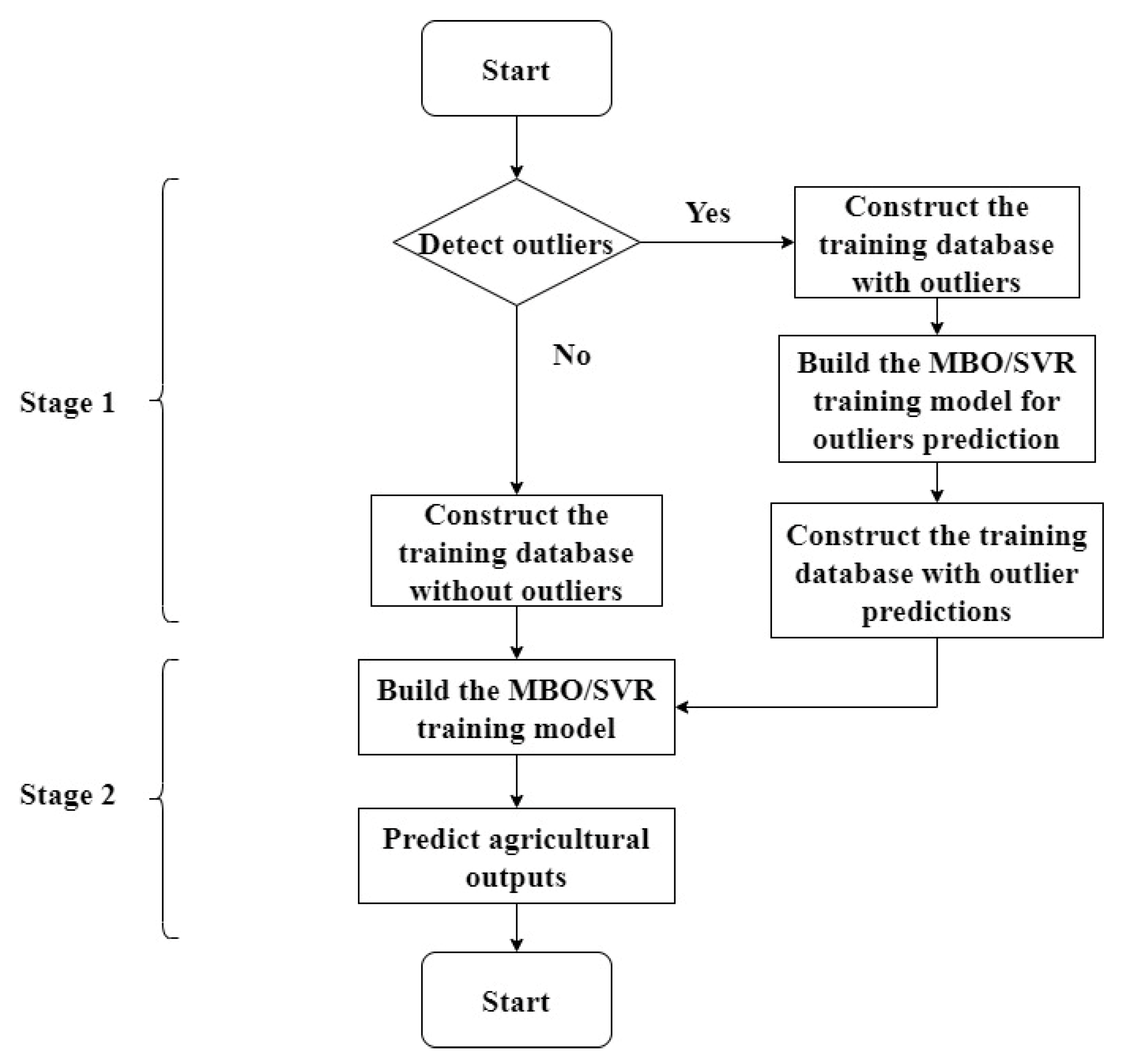
The MBO/SVR model comprises two main stages. Stage 1 is the data pre-processing stage for the training model, and Stage 2 is the prediction stage for agricultural output data prediction. Figure 3 shows the flowchart of the MOB/SVR model. The detailed algorithm of the MBO/SVR model can be introduced as follows.

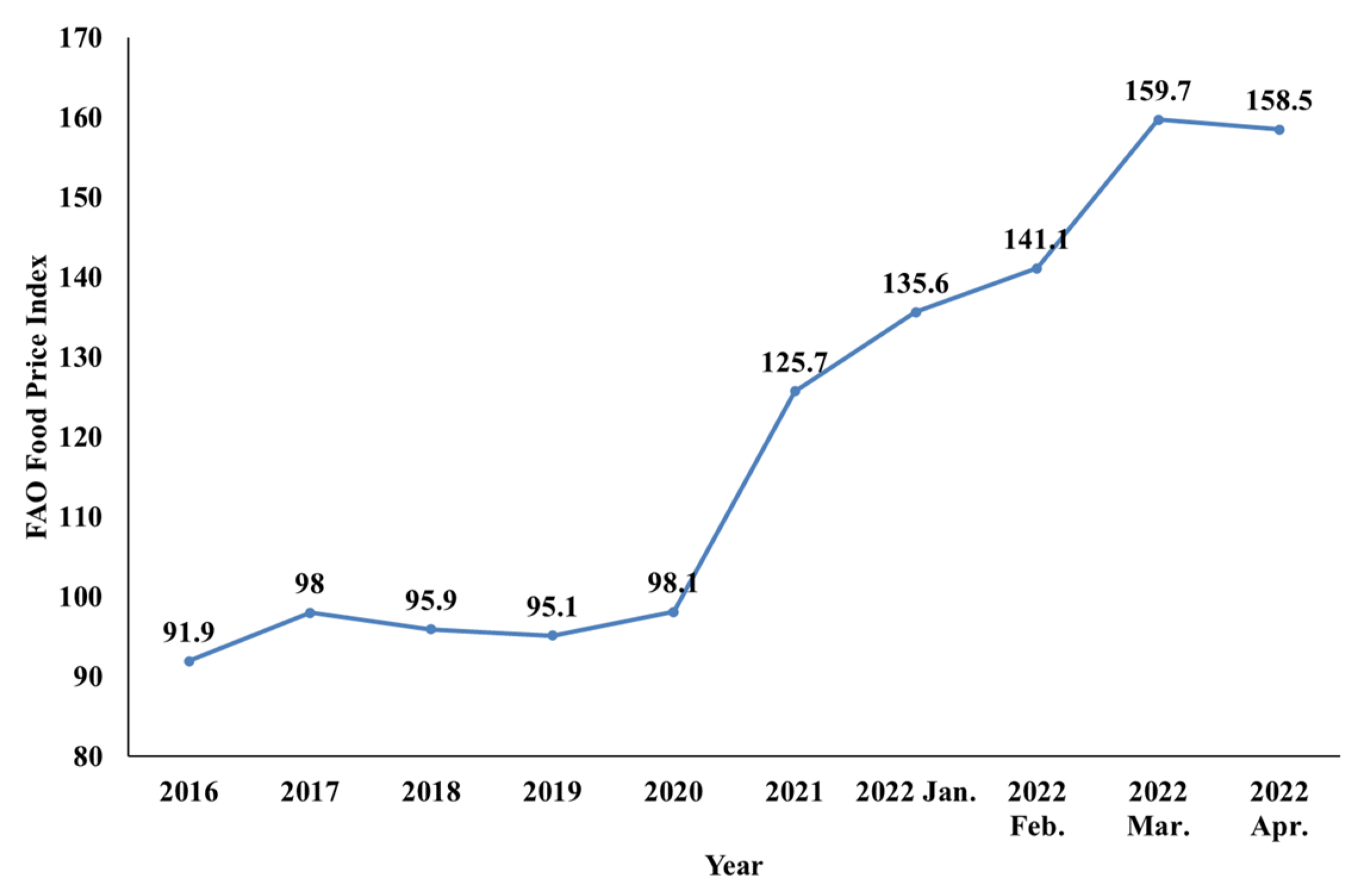
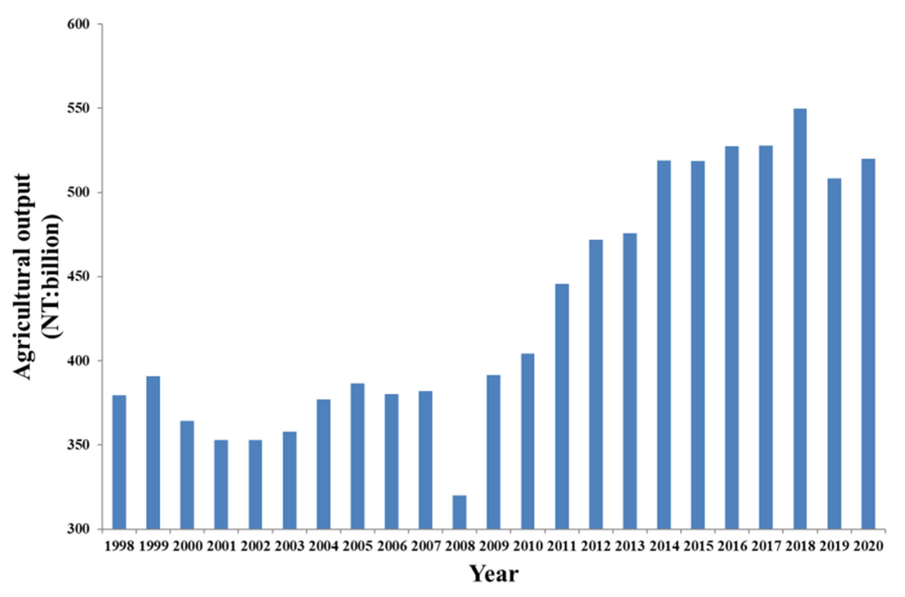
• Stage 1

As described in Section 2.1, the annual total agricultural output data have been highly volatile in recent years. Therefore, predictions must detect and smooth outlier data [42]. Accordingly, the main goal of Stage 1 is detecting outlier data and reducing their effects when building the prediction model. There are two major steps in Stage 1.

Step 1: Detect outliers

First, we standardize the data based on Equation (6), where x_i denotes the ith datum; $\overline{x}$ and SD denote the mean and the standard deviation of the dataset, respectively; and z_i denotes the z-score of the ith datum of the training dataset. This study used a critical value for the outlier of ±2; i.e., when the ith z-score is greater than 2 or less than −2, the ith datum is an outlier. Subsequently, when there are no outliers in the training dataset, go to Step 2 to construct the training database without outliers; otherwise, go to Step 2.1 to construct the training database with outliers.

$$z_i=\frac{x_i-\overline{x}}{SD}.$$

(6)

Step 2: Construct the training database without outliers

When there are no outliers in the dataset, the training database can be constructed without outliers the MBO/SVR training model can be built in Step 3. Data volatility affects the training model’s performance regardless of whether outliers are detected. Accordingly, the actual data must be transformed based on Equation (7) before constructing the training database. In Equation (7), T_t denotes the tth transformed datum, and A_t and A_t−1 are the actual tth and (t − 1)th data, respectively.

$$T_t=(A_t-A_{t-1})/A_{t-1},where t>1.$$

(7)

We can provide a simple example to describe the process of constructing the training database. Suppose a dataset includes ten years’ annual total agricultural output data;

Table 1. An example of actual and transformed data.

	Year1	Year2	Year3	Year4	…	Year9	Year10
Actual data	A1	A2	A3	A4	…	A9	A10
Transformed data		T2	T3	T4	…	T9	T10

shows the actual and transformed data according to Equation (7). The training database can be constructed as shown in

Table 2. An example of a training database without outliers.

Training ID	Input Variable (X)	Output Variable (Y)
1	T2	T3
2	T3	T4
3	T4	T5
4	T5	T6
5	T6	T7
6	T7	T8
7	T8	T9
8	T9	T10

. In Table 2, each training ID denotes a sample, and the input variable (X) and output variable (Y) are fed into the MBO/SVR model to build the training model. When constructing the training database, go to Step 3 to build the MBO/SVR training model.

Step 2.1: Construct the training database with outliers

As described in Step 2, the actual annual total agricultural output data must be transformed using Equation (7) to reduce the effect of data volatility whether outliers are detected or not. Therefore, when outliers are detected, Table 1 must still be constructed. As the agricultural output data are presented in a time-series dataset, prediction of future values should be based on previously observed values [40,41,43,44]. Accordingly, parts of the data should be removed to construct the training database for the training model. For example, suppose the Year₃ data in Table 1 is detected as outlier data. Then, T₃ and T₄ will be removed because they were caused by Year₃ data. Therefore, the data with training IDs 1 to 3 in Table 2 are also released.

Table 3. An example of a training database with outliers.

Training ID	Input Variable (X)	Output Variable (Y)
4	T5	T6
5	T6	T7
6	T7	T8
7	T8	T9
8	T9	T10

shows the constructed training database with outliers.

Step 2.2: Build the MBO/SVR training model for outlier prediction

Step 2.2 involves building the MBO/SVR training model for outlier prediction using the training database with outliers. As the central concept of the MBO/SVR model is searching for the best and most suitable parameter setting in the SVR model by using the MBO algorithm to enhance the performance, the procedures of the MBO/SVR model for outlier prediction include two steps, as described in Step 2.2.1 and Step 2.2.2.

Step 2.2.1: Set the initial queen of the MBO

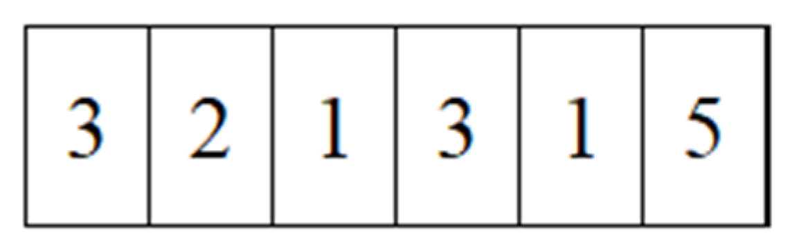
The queen of the MBO refers to a candidate parameter setting in the MBO/SVR model. A queen is coded as an integer sequence with six spermathecae. The first three spermathecae indicate a candidate solution for the Cost parameter of the SVR model; the remainders are candidate solutions for the Gamma parameter of the SVR model. Figure 4 shows an example of a queen. As the Cost parameter is set between 0 and 10, the first three spermathecae (321) in Figure 4 indicate that the Cost parameter is set to 3.21. Similarly, because the Gamma parameter is set between 0 and 1, the remaining spermatheca (315) in Figure 4 indicate that the Gamma parameter is set to 0.315. Subsequently, the parameter settings build the training MBO/SVR model. The fitness function of the MBO/SVR model is defined by Equations (8) and (9). In Equations (8) and (9), $\widehat{T_t}$ and $\widehat{A_t}$ denote the t^th predicted transformed agricultural output datum and the t^th predicted agricultural output datum, respectively; A_t denotes the t^th actual agricultural output data; and n denotes the number of predictions.

$$\widehat{A_t}=\widehat{T_t}{\times A}_{t-1}{+A}_{t-1}.$$

(8)

$$fitness function=\left(\frac{1}{n}{{\displaystyle \sum }}_{t=1}^n\frac{\left|A_t-{\widehat{A}}_t\right|}{A_t}\right).$$

(9)

Step 2.2.2: Complete the mating flight of the MBO

To search for the optimization solution, the MBO algorithm generates the next generation of broods through a mating flight. After completing the mating flight of the MBO algorithm, many broods will have been generated. We then calculate the fitness values of the broods. When a brood’s fitness value is better than the queen’s fitness value, the queen will be replaced with the brood.

There are two termination conditions in the MBO/SVR model: (a) when the last 50 generations’ fitness values are the same, the best queen is selected as the best parameter setting in the MBO/SVR model; (b) when the number of generations is greater than 500, the best queen is selected as the best parameter setting in the MBO/SVR model.

Step 2.3: Build the MBO/SVR training model for outlier prediction

When terminating the algorithm, the best queen is selected as the best parameter setting in the MBO/SVR model. Subsequently, the input variables (X) and output variables (Y) in the training database with outliers are fed into the MBO/SVR model to build the training model for outlier prediction. As the example in Step 2.1 shows, the Year₃ in Table 1 is detected as outlier data. T₂ is fed into the training MBO/SVR model to predict the output value ${\widehat{T}}_3$ and to replace T₃ with ${\widehat{T}}_3$. Subsequently, ${\widehat{A}}_3$ and ${\widehat{T}}_4$ can be calculated by ${\widehat{T}}_3$ according to Equations (7) and (8).

Step 2.4: Construct the training database with outlier predictions

After Step 2.3, we use the outlier predictions to construct the training database with outlier predictions according to the same approach as in Step 2.

Table 4. An example of a training database with outlier predictions.

Training ID	Input Variable (X)	Output Variable (Y)
1	T2	${\widehat{T}}_3$
2	${\widehat{T}}_3$	${\widehat{T}}_4$
3	${\widehat{T}}_4$	T5
4	T5	T6
5	T6	T7
6	T7	T8
7	T8	T9
8	T9	T10

shows the results for the training database with outlier predictions according to the example in Step 2.1.

• Stage 2

Step 3: Build the MBO/SVR training model

After constructing the training database, we then use it to build the MBO/SVR training model. The procedure for building the MBO/SVR training model is the same as in Step 2.2. The MBO/SVR training model also needs to search for the best and most suitable parameter setting in the SVR model with the MBO algorithm.

Step 4: Predict agricultural outputs

Once the MBO/SVR training model has been built, we predict the agricultural outputs by feeding the test data into the MBO/SVR model. The procedure for prediction is the same as in Step 2.3.

2.5. Performance Measures

Three performance measures were used to verify prediction accuracy: the mean absolute percentage error (MAPE), the root mean square percentage error (RMSPE), and the relative root mean squared error (r-RMSE). Ahlburg [45] indicates that the MAPE and the RMSPE can help in comparing various prediction models, and they have been widely used for measuring prediction accuracy [21,44]. The MAPE and RMSPE are defined in Equations (10) and (11), where t denotes the tth data point (t = 1, 2, 3, …, and n), n represents the number of predicted values, and A_t and ${\widehat{A}}_t$ denote the tth actual and the tth predicted value, respectively.

$$MAPE=\left(\frac{1}{n}{{\displaystyle \sum }}_{t=1}^n\frac{\left|A_t-{\widehat{A}}_t\right|}{A_t}\right)\times 100,$$

(10)

$$RMSPE=\sqrt{\frac{1}{n}{{\displaystyle \sum }}_{t=1}^n{\left(\frac{A_t-{\widehat{A}}_t}{A_t}\right)}^2}\times 100.$$

(11)

Furthermore, the r-RMSE is also widely applied in many fields [16,46,47] because it can be used to compare the performances of different models. The calculations for the r-RMSE are defined in Equation (12), where $\overline{A}$ denotes the average of the actual data. A lower MAPE, RMSPE, or r-RMSE value indicates that a model has a more accurate prediction performance.

$$r-RMSE=\frac{1}{\overline{A}}\times \sqrt{\frac{1}{n}\times {{\displaystyle \sum }}_{t=1}^n{(A_t-{\widehat{A}}_t)}^2}\times 100.$$

(12)

As well as using MAPE, RMSPE, and r-RMSE to verify the prediction accuracy of the models, this study also used directional symmetry (DS) to measure the coincidence in the prediction direction trends between the predicted and the actual values [48]. The DS is defined by Equation (13):

$$\mathrm{DS}=\frac{1}{n-1}{{\displaystyle \sum }}_{t=2}^n{d}_t\times 100\%, \mathrm{where} d_t=\{\begin{array}{cc}1,& \mathrm{if} \left(A_t-A_{t-1}\right)\times \left({\widehat{A}}_t-{\widehat{A}}_{t-1}\right)>0\\ 0,& \mathrm{otherwise}\end{array}.$$

(13)

2.6. Performance Testing

Traditionally performance measures are used to evaluate prediction models’ accuracy. However, the traditional prediction evaluation criteria have limitations in their applications to some cases [49]. Moreover, most research has only used the results of performance measures to compare which model is better without statistical testing.

The Diebold–Mariano test was first proposed in 1995 [50]. The Diebold–Mariano test is used to test the prediction performance of different models [44,49]. The procedure for the Diebold–Mariano test is described in the following.

Suppose $y_t$ and ${\widehat{y}}_{i,t}$ denote the tth actual time-series data point and the tth predicted time-series data point of the ith competing prediction model, respectively. Subsequently, $e_{i,t}$ (i = 1, 2, 3,…, m) denotes the tth prediction error of the ith competing prediction model, where m denotes the number of competing models. The tth prediction error $e_{i,t}$ is defined by Equation (14):

$$e_{i,t}=y_t-{\widehat{y}}_{i,t}, where i=1,2,3,...,m$$

(14)

The accuracy of each prediction model can be measured according to the loss function, as shown in Equation (15):

$$L\left(y_t,{\widehat{y}}_{i,t}\right)=L\left(e_{i,t}\right).$$

(15)

Generally, the most widely used loss functions are the squared-error and absolute-error functions. Their equations are shown in Equations (16) and (17), respectively:

$$L\left(y_t,{\widehat{y}}_{i,t}\right)=L\left(e_{i,t}\right)={{\displaystyle \sum }}_{t=1}^T{(e_{i,t})}^2,$$

(16)

$$L\left(y_t,{\widehat{y}}_{i,t}\right)=L\left(e_{i,t}\right)={{\displaystyle \sum }}_{t=1}^T{\left|e_{i,t}\right|}^2.$$

(17)

Finally, the hypothesis of the Diebold–Mariano test can be used to test the accuracy of prediction models. The hypothesis is given as follows:

$$H_0:E\left[L\left(e_{1,t}\right)\right]=E\left[L\left(e_{2,t}\right)\right] \mathrm{vs}. H_1:E\left[L\left(e_{1,t}\right)\right]\ne E\left[L\left(e_{2,t}\right)\right]$$

3. Results

3.1. Comparison Models

Four prediction models, including the linear regression model (LM), the GA-based improved GM(1,1) (GAIGM(1, 1)) model, the artificial neural network (ANN) model, and the long short-term memory (LSTM) model, were evaluated and their performances to that of the MBO/SVR model. The LM and the ANN model are well-known models in statistics and artificial intelligence, respectively. The GAIGM(1, 1) model was proposed to enhance the performance of the improved GM(1,1) model for agricultural output prediction [21]. The LSTM model has been a popular deep-learning model in recent years.

The LM is implemented with R language in this study, and the GAIGM(1, 1) model parameters were set according to the literature [21]. Therefore, this study estimated the GAIGM(1, 1) model parameters as a = −0.006727 and b = 358.1945; the ANN model was implemented with the default parameter setting from the “RSNNS” package of the R language; the LSTM model was implemented with the default parameter setting from the “keras” package of the Python language.

3.2. Experimental Results

In this study, the parameters of the MBO algorithm were set as in

Table 5. Parameters of the MBO algorithm.

Parameters	Settings
Number of workers	10
Number of broods	10
Initial energy of queen	100
Initial speed of queen	100

. We first performed outlier detection in Step 1 of the MBO/SVR model. As the z-score of the actual data in 2008 was less than −2, the data were regarded as outlier data. In accordance with the MBO/SVR model’s algorithm, the data from 2008 had to be removed and the predicted data used to construct the training database. Subsequently, the MBO/SVR model predicted the data value in 2008 as 387.9. Therefore, this value (387.9) was used to replace the data in 2008 to build the MBO/SVR model.

Table 6. Comparison of the models’ performances.

	LM	GAIGM(1, 1)	ANN	LSTM	MBO/SVR
Training MAPE(%)	4.31	4.35	3.85	4.28	3.72 *
MAPE(%)	18.96	18.15	22.81	19.82	3.77 *
RMAE(%)	19.68	19.67	24.28	20.60	4.90 *
r-RMSE(%)	20.60	20.80	25.61	21.58	4.85 *
DS(%)	52.38	61.90	47.62	52.38	65.00 *

* denotes the best value among all models.

shows the experiment results. The MAPE was used for the training models’ performance comparison because the MBO/SVR model uses the MAPE as the fitness function. The other performance measures in Table 6 were used to compare the performance with the test dataset. According to Table 6, the training MAPE ranged from 3.72 to 4.35. The training performances of the models were similar according to the training MAPE. However, the training performance of the ANN and the MBO/SVR models should be better than the other models because only their training MAPEs were less than 4. For the test dataset, the MAPE ranged from 3.77 to 22.81; the RMAE ranged from 4.90 to 24.28; and the r-RMSE ranged from 4.85 to 25.61. Furthermore, only the MBO/SVR and GAIGM(1, 1) models’ DS values were greater than 60%. According to the results, the models’ performances were similar in terms of MAPE, RMAE, r-RMSE, and DS, whether they were statistical, machine-learning, or artificial-intelligence models. Only the MBO/SVR model demonstrated a robust performance, and it also had the best performance.

4. Discussion

In accordance with a definition from the literature [51], the MBO/SVR model was the only model with highly accurate predictive power because only this model had a MAPE was lower than 10%. Hence, the MBO/SVR model demonstrated the optimal performance according to the MAPE, RMSPE, r-RMSE, and DS results, as shown in Table 6. The MAPE, RMSPE, and r-RMSE for the MBO/SVR model were approximately 75% lower than the other models. However, the results still had to be verified with statistical testing. Therefore, this study used the Diebold–Mariano test to provide statistical verification. The results for the Diebold–Mariano test are shown in

Table 7. The Diebold–Mariano test for the models.

	LM	GAIGM(1, 1)	ANN	LSTM
LM
GAIGM(1, 1)	−1.66 (p-value = 0.12)
ANN	−3.82 (p-value < 0.01 *)	−3.97 (p-value < 0.01 *)
LSTM	−4.04 (p-value < 0.01 *)	−1.83 (p-value = 0.09)	3.77 (p-value < 0.01 *)
MBO/SVR	3.82 (p-value < 0.01 *)	3.67 (p-value < 0.01 *)	3.88 (p-value < 0.01 *)	3.87 (p-value < 0.01 *)

Note: the numbers in the table are the statistics from the Diebold–Mariano test; * denotes significance at α = 0.05.

. Obviously, the MBO/SVR model was significantly better than the other models; the LM and GAIGM(1, 1) model were insignificantly different, but the LM was significantly better than the LSTM and ANN models. The LSTM model was significantly better than the ANN model. Accordingly, based on the results of the Diebold–Mariano test and the DS, the rank for the performances for the agricultural output data was as shown in the following:

MBO/SVR > GAIGM(1, 1) > LSTM ≥ LM > ANN.

Although the Diebold–Mariano test could test the models’ performances differently, the models’ prediction trends also had to be confirmed. Figure 5 and Table S1 show the actual agricultural output data and the prediction results from the models. For the training dataset, the trends for the prediction results for all models were close to the actual training data. However, the MBO/SVR model prediction trend was the only one consistent with the test dataset. The other models could not predict the volatility of the agricultural output. Accordingly, the MBO/SVR is a robust long-term agricultural output prediction model.

The model performance results from this study are similar to those from the literature [5,14,52,53,54]: (a) the performance of the SVR-based model was better than the traditional linear model (i.e., linear regression model), and (b) the models must frequently be retrained to enhance the prediction performance when the range of the test dataset exceeds the training dataset, especially if the dataset is a data stream or time series. Therefore, the MBO/SVR model can be successfully and suitably applied to agricultural output prediction issues because it demonstrates the best performance, especially for predicting long-term agricultural output without retraining the prediction model. Furthermore, compared to results from studies [21] using similar agricultural output data, the MBO/SVR model is more effective in avoiding the influence of outliers in agricultural output as it uses the robustness model for long-term agricultural output prediction.

5. Conclusions

5.1. Research Contributions

Implementing an effective agricultural output prediction model is essential in agricultural policymaking and could potentially solve food crises. This study proposed the MBO/SVR model to solve two major problems relating to agricultural output data. Moreover, the performance of the MBO/SVR model was compared with the performances of four models by using the agricultural output data from 1998 to 2020 from Taiwan. The experimental results for the MAPE, RMSPE, r-RMSE, and DS indicated that the prediction performance of the MBO/SVR model was more favorable than that of the other models. The MAPE, RMSPE, and r-RMSE of the MBO/SVR model were approximately 75% lower than for the other models. Furthermore, by using the Diebold–Mariano test, the performance of the MBO/SVR model was found to be significantly better than the other models at α = 0.05. Additionally, only the MBO/SVR model achieved a DS value of 60%; i.e., the MBO/SVR model could predict coincidences in the prediction direction trends between the predicted and the actual values. Moreover, only the MBO/SVR model had a prediction trend that was consistent with the actual agricultural output data for the test dataset, especially for the prediction of the long-term agricultural output.

According to the results, the MBO/SVR model can directly apply agricultural output data to avoid statistical assumptions and reduce the frequency of model retraining. Furthermore, the MBO/SVR model offers two advantages: (a) it can automatically locate outlier data and minimize the effects of outlier data for the training model, and (b) it is a robust model for predicting long-term agricultural output without retraining the model because it can satisfy different conditions. Accordingly, the MBO/SVR model is suitable for agricultural output prediction. Therefore, the MBO/SVR model should also be used to assist governments in developing good agricultural policies.

5.2. Research Limitations and Future Research

In this study, the annual total agricultural output from 1998 to 2020 was collected from the Agricultural Statistics Yearbook Annual Report of the Council of Agriculture, Executive Yuan of Taiwan. As the dataset only includes 23 years, this might have affected and limited the performances of the machine-learning or AI models. Therefore, we provide the following suggestions for future research: (a) the data collection period should be extended because it might affect the training models’ prediction performances; (b) the MBO/SVR model should be integrated with precision agriculture technologies [3,4], such as the Internet of Things (IoT), because this would help in obtaining various real-time data; and (c) by integrating precision agriculture technologies, the MBO/SVR model could be made to include more variables, such as climate data, since many external factors can affect agricultural data.

References

1. FAO. FAO Food Price Index. Available online: https://www.fao.org/worldfoodsituation/foodpricesindex/en/ (accessed on 1 July 2022).
2. European Council Council of the European Union. Food Security and Affordability. Available online: https://www.consilium.europa.eu/en/policies/food-security-and-affordability/ (accessed on 1 July 2022).
3. Scuderi, A.; La Via, G.; Timpanaro, G.; Sturiale, L. The Digital Applications of “Agriculture 4.0”: Strategic Opportunity for the Development of the Italian Citrus Chain. Agriculture 2022, 12, 400. [Google Scholar] [CrossRef]
4. Cheng, Z.; Lu, Z. Regression-Based Correction and I-PSO-Based Optimization of HMCVT’s Speed Regulating Characteristics for Agricultural Machinery. Agriculture 2022, 12, 580. [Google Scholar] [CrossRef]
5. Sun, Y.; Zhang, S.; Tao, F.; Aboelenein, R.; Amer, A. Improving Winter Wheat Yield Forecasting Based on Multi-Source Data and Machine Learning. Agriculture 2022, 12, 571. [Google Scholar] [CrossRef]
6. Priyadarshini, P.; Abhilash, P.C. Agri-food systems in India: Concerns and policy recommendations for building resilience in post COVID-19 pandemic times. Glob. Food Secur. 2021, 29, 100537. [Google Scholar] [CrossRef]
7. Marengo, J.A.; Galdos, M.V.; Challinor, A.; Cunha, A.P.; Marin, F.R.; Vianna, M.d.S.; Alvala, R.C.S.; Alves, L.M.; Moraes, O.L.; Bender, F. Drought in Northeast Brazil: A review of agricultural and policy adaptation options for food security. Clim. Resil. Sustain. 2022, 1, e17. [Google Scholar] [CrossRef]
8. Pang, J.; Li, X.; Li, X.; Yang, T.; Li, Y.; Chen, X. Analysis of Regional Differences and Factors Influencing the Intensity of Agricultural Water in China. Agriculture 2022, 12, 546. [Google Scholar] [CrossRef]
9. Chang, T.Y. The influence of agricultural policies on agriculture structure adjustment in Taiwan. China Agric. Econ. Rev. 2011, 3, 67–79. [Google Scholar] [CrossRef]
10. Darekar, A.; Reddy, A.A. Cotton price forecasting in major producing states. Econ. Aff. 2017, 62, 373–378. [Google Scholar] [CrossRef]
11. Assis, K.; Amran, A.; Remali, Y. Forecasting cocoa bean prices using univariate time series models. Res. World 2010, 1, 71. [Google Scholar]
12. Gu, Y.H.; Jin, D.; Yin, H.; Zheng, R.; Piao, X.; Yoo, S.J. Forecasting Agricultural Commodity Prices Using Dual Input Attention LSTM. Agriculture 2022, 12, 256. [Google Scholar] [CrossRef]
13. Lee, C.-P.; Shieh, G.-J.; Yiu, T.-J.; Kuo, B.-J. The strategy to simulate the cross-pollination rate for the co-existence of genetically modified (GM) and non-GM crops by using FPSOSVR. Chemom. Intell. Lab. Syst. 2013, 122, 50–57. [Google Scholar] [CrossRef]
14. Jheng, T.; Li, T.; Lee, C. Using Hybrid Support Vector Regression to Predict Agricultural Output. In Proceedings of the 27th Wireless and Optical Communication Conference (WOCC), Hualien, Taiwan, 30 April–1 May 2018; pp. 1–3. [Google Scholar]
15. Liu, L.-W.; Hsieh, S.-H.; Lin, S.-J.; Wang, Y.-M.; Lin, W.-S. Rice Blast (Magnaporthe oryzae) Occurrence Prediction and the Key Factor Sensitivity Analysis by Machine Learning. Agronomy 2021, 11, 771. [Google Scholar] [CrossRef]
16. Liu, L.-W.; Lu, C.-T.; Wang, Y.-M.; Lin, K.-H.; Ma, X.; Lin, W.-S. Rice (Oryza sativa L.) Growth Modeling Based on Growth Degree Day (GDD) and Artificial Intelligence Algorithms. Agriculture 2022, 12, 59. [Google Scholar] [CrossRef]
17. Castro, C.A.d.O.; Resende, R.T.; Kuki, K.N.; Carneiro, V.Q.; Marcatti, G.E.; Cruz, C.D.; Motoike, S.Y. High-performance prediction of macauba fruit biomass for agricultural and industrial purposes using Artificial Neural Networks. Ind. Crops Prod. 2017, 108, 806–813. [Google Scholar] [CrossRef]
18. Shen, Y.; Mercatoris, B.; Cao, Z.; Kwan, P.; Guo, L.; Yao, H.; Cheng, Q. Improving Wheat Yield Prediction Accuracy Using LSTM-RF Framework Based on UAV Thermal Infrared and Multispectral Imagery. Agriculture 2022, 12, 892. [Google Scholar] [CrossRef]
19. Tian, H.; Wang, P.; Tansey, K.; Zhang, J.; Zhang, S.; Li, H. An LSTM neural network for improving wheat yield estimates by integrating remote sensing data and meteorological data in the Guanzhong Plain, PR China. Agric. For. Meteorol. 2021, 310, 108629. [Google Scholar] [CrossRef]
20. Haider, S.A.; Naqvi, S.R.; Akram, T.; Umar, G.A.; Shahzad, A.; Sial, M.R.; Khaliq, S.; Kamran, M. LSTM Neural Network Based Forecasting Model for Wheat Production in Pakistan. Agronomy 2019, 9, 72. [Google Scholar] [CrossRef] [Green Version]
21. Ou, S.-L. Forecasting agricultural output with an improved grey forecasting model based on the genetic algorithm. Comput. Electron. Agric. 2012, 85, 33–39. [Google Scholar] [CrossRef]
22. Rajula, H.S.R.; Verlato, G.; Manchia, M.; Antonucci, N.; Fanos, V. Comparison of Conventional Statistical Methods with Machine Learning in Medicine: Diagnosis, Drug Development, and Treatment. Medicina 2020, 56, 455. [Google Scholar] [CrossRef]
23. Chen, X.-Z.; Chang, C.-M.; Yu, C.-W.; Chen, Y.-L. A Real-Time Vehicle Detection System under Various Bad Weather Conditions Based on a Deep Learning Model without Retraining. Sensors 2020, 20, 5731. [Google Scholar] [CrossRef]
24. Klabjan, D.; Zhu, X. Neural Network Retraining for Model Serving. arXiv 2020, arXiv:2004.14203. [Google Scholar]
25. Drucker, H.; Burges, C.J.C.; Kaufman, L.; Smola, A.; Vapnik, V. Support Vector Regression Machines. In Proceedings of the 9th International Conference on Neural Information Processing Systems, Denver, CO, USA, 3–5 December 1996; pp. 155–161. [Google Scholar]
26. Lee, C.-P. Reduced the Risk in Agriculture Management for Government Using Support Vector Regression with Dynamic Optimization Parameters. Lex Localis 2017, 15, 243–261. [Google Scholar] [CrossRef]
27. Tian, Y.; Xu, Y.-P.; Wang, G. Agricultural drought prediction using climate indices based on Support Vector Regression in Xiangjiang River basin. Sci. Total Environ. 2018, 622–623, 710–720. [Google Scholar] [CrossRef] [PubMed]
28. Alotaibi, M. Hybrid metaheuristic technique for optimal container resource allocation in cloud. Comput. Commun. 2022, 191, 477–485. [Google Scholar] [CrossRef]
29. Li, L.; Vyth, J. Effects of Different Worker Heuristics in Marriage in Honey Bees Optimization: As Applied to the Graph Coloring Problem. Bachelor’s Thesis, KTH Royal Institute of Technology, Stockholm, Sweden, June 2018. [Google Scholar]
30. Prabhakar, S.K.; Lee, S. Transformation Based Tri-Level Feature Selection Approach Using Wavelets and Swarm Computing for Prostate Cancer Classification. IEEE Access 2020, 8, 127462–127476. [Google Scholar] [CrossRef]
31. COA. Agricultural Statistics Yearbook. Available online: https://agrstat.coa.gov.tw/sdweb/public/book/Book.aspx (accessed on 1 July 2022).
32. Abbass, H.A. MBO: Marriage in Honey Bees Optimization—A Haplometrosis Polygynous Swarming Approach. In Proceedings of the 2001 Congress on Evolutionary Computation (IEEE Cat. No.01TH8546), Seoul, Korea, 27–30 May 2001; Volume 201, pp. 207–214. [Google Scholar]
33. Curkovic, P.; Jerbic, B. Honey-Bees Optimization Algorithm Applied to Path Planning Problem. Int. J. Simul. Model. 2007, 6, 154–164. [Google Scholar] [CrossRef]
34. Celik, Y.; Ulker, E. An Improved Marriage in Honey Bees Optimization Algorithm for Single Objective Unconstrained Optimization. Sci. World J. 2013, 2013, 370172. [Google Scholar] [CrossRef]
35. Celik, Y.; Ülker, E. A marriage in honey bee Ooptimisation approach to the asymmetric Travelling salesman problem. Int. J. Innov. Comput. Inf. Control. 2012, 8, 4123–4132. [Google Scholar]
36. Fung, K.F.; Huang, Y.F.; Koo, C.H.; Mirzaei, M. Improved SVR machine learning models for agricultural drought prediction at downstream of Langat River Basin, Malaysia. J. Water Clim. Change 2019, 11, 1383–1398. [Google Scholar] [CrossRef]
37. Ceylan, Z. Assessment of agricultural energy consumption of Turkey by MLR and Bayesian optimized SVR and GPR models. J. Forecast. 2020, 39, 944–956. [Google Scholar] [CrossRef]
38. Shengwei, W.; Yanni, L.; Jiayu, Z.; Jiajia, L. Agricultural price Fluctuation Model Based on SVR. In Proceedings of the 2017 9th International Conference on Modelling, Identification and Control (ICMIC), Kunming, China, 10–12 July 2017; pp. 545–550. [Google Scholar]
39. Niu, P.; Zhang, W. Model of turbine optimal initial pressure under off-design operation based on SVR and GA. Neurocomputing 2012, 78, 64–71. [Google Scholar] [CrossRef]
40. Huang, C.-H.; Yang, F.-H.; Lee, C.-P. The strategy of investment in the stock market using modified support vector regression model. Sci. Iran. 2018, 25, 1629–1640. [Google Scholar] [CrossRef] [Green Version]
41. Liu, J.; Hu, Y.X. Support Vector Regression with Kernel Mahalanobis Measure for Financial Forecast. Intell. Syst. Ref. Libr. 2013, 47, 215–227. [Google Scholar] [CrossRef]
42. Kordos, M.; Rusiecki, A. Reducing noise impact on MLP training. Soft Comput. 2016, 20, 49–65. [Google Scholar] [CrossRef] [Green Version]
43. Lee, C.-P.; Lin, W.-C.; Yang, C.-C. A strategy for forecasting option price using fuzzy time series and least square support vector regression with a bootstrap model. Sci. Iran. 2014, 21, 815–825. [Google Scholar]
44. Yang, C.-C.; Leu, Y.; Lee, C.-P. A Dynamic Weighted Distancedbased Fuzzy Time Series Neural Network with Bootstrap Model for Option Price Forecasting. Rom. J. Econ. Forecast. 2014, 2014, 115–129. [Google Scholar]
45. Ahlburg, D.A. How Accurate are the U.S. Bureau of the Census Projections of Total Live Births? J. Forecast. 1982, 1, 365–374. [Google Scholar] [CrossRef]
46. Cao, L.; Liu, H.; Fu, X.; Zhang, Z.; Shen, X.; Ruan, H. Comparison of UAV LiDAR and Digital Aerial Photogrammetry Point Clouds for Estimating Forest Structural Attributes in Subtropical Planted Forests. Forests 2019, 10, 145. [Google Scholar] [CrossRef] [Green Version]
47. Liu, L.-W.; Wang, Y.-M. Modelling Reservoir Turbidity Using Landsat 8 Satellite Imagery by Gene Expression Programming. Water 2019, 11, 1479. [Google Scholar] [CrossRef] [Green Version]
48. Leu, Y.; Lee, C.-P.; Jou, Y.-Z. A distance-based fuzzy time series model for exchange rates forecasting. Expert Syst. Appl. 2009, 36, 8107–8114. [Google Scholar] [CrossRef]
49. Chen, H.; Wan, Q.; Wang, Y. Refined Diebold-Mariano Test Methods for the Evaluation of Wind Power Forecasting Models. Energies 2014, 7, 4185–4198. [Google Scholar] [CrossRef] [Green Version]
50. Diebold, F.X.; Mariano, R.S. Comparing Predictive Accuracy. J. Bus. Econ. Stat. 1995, 13, 253–263. [Google Scholar] [CrossRef] [Green Version]
51. DeLurgio, S.A. Forecasting Principles and Applications, 1st ed.; Irwin/McGraw-Hill: New York, NY, USA, 1998. [Google Scholar]
52. Aworka, R.; Cedric, L.S.; Adoni, W.Y.H.; Zoueu, J.T.; Mutombo, F.K.; Kimpolo, C.L.M.; Nahhal, T.; Krichen, M. Agricultural decision system based on advanced machine learning models for yield prediction: Case of East African countries. Smart Agric. Technol. 2022, 2, 100048. [Google Scholar] [CrossRef]
53. Parviz, L. Assessing accuracy of barley yield forecasting with integration of climate variables and support vector regression. Ann. Univ. Mariae Curie-Sklodowska Sect. C Biol. 2019, 73, 19–30. [Google Scholar] [CrossRef]
54. Ksieniewicz, P.; Woźniak, M.; Cyganek, B.; Kasprzak, A.; Walkowiak, K. Data stream classification using active learned neural networks. Neurocomputing 2019, 353, 74–82. [Google Scholar] [CrossRef]
Figure 1. FAO Food Price Index from 2016 to 2022 April.
Agriculture 12 01075 g001
Figure 2. The annual total agricultural output from 1998 to 2020 in Taiwan.
Agriculture 12 01075 g002
Figure 3. The flowchart of the MBO/SVR model.
Agriculture 12 01075 g003
Figure 4. An example of the phenotype of a queen.
Agriculture 12 01075 g004
Figure 5. The prediction results of the models.
Agriculture 12 01075 g005