Assessing Machine Learning-Based Prediction under Different Agricultural Practices for Digital Mapping of Soil Organic Carbon and Available Phosphorus

Abstract

Predicting soil chemical properties such as soil organic carbon (SOC) and available phosphorus (Ava-P) content is critical in areas where different land uses exist. The distribution of SOC and Ava-P is influenced by both natural and anthropogenic factors. This study aimed at (1) predicting SOC and Ava-P in a piedmont plain of Northeast Iran using the Random Forests (RF) and Cubist mathematical models and hybrid models (Regression Kriging), (2) comparing the models’ results, and (3) identifying the key variables that influence the spatial dynamics of soil SOC and Ava-P under different agricultural practices. The machine learning models were trained with 201 composite surface soil samples and 24 ancillary data, including climate (C), organism (O), topography- relief (R), parent material (P) and key soil features (S) according to the SCORPAN digital soil mapping framework, which can predictively represent soil formation factors spatially. Clay, one of the most critical soil properties with a well-known relationship to SOC, was the most important predictor of SOC, followed by open-access multispectral satellite images-based vegetation and soil indices. Ava-P had a similar set of effective variables. Hybrid approaches did not improve model accuracy significantly, but they did reduce map uncertainty. In the validation set, Ava-P was calculated using the RF algorithm with a normalized root mean square (NRMSE) of 96.8, while SOC was calculated using the Cubist algorithm with an NRMSE of 94.2. These values did not change when using the hybrid technique for Ava-P; however, they changed just by 1% for SOC. The management of SOC content and the supply of Ava-P in agricultural activities can be guided by SOC and Ava-P digital distribution maps. Produced digital maps in which the soil scientist plays an active role can be used to identify areas where concentrations are high and need to be protected, where uncertainty is high and sampling is required for further monitoring.

1. Introduction

The spatial prediction of soil properties plays an essential role in agricultural production and sustainable land management [1,2,3,4]. The spatial variability of soil properties is influenced by soil formation factors such as climate, time, parent material, topography, and vegetation as defined by Jenny [5] but also is mainly influenced by anthropogenic activities [6,7,8]. The agricultural productivity of soils in arid and semi-arid regions may vary significantly over short distances under the influence of human factors. Within the framework of digital soil mapping, soil scientists are working on the most accurate spatial mapping of soil properties in areas where human influences are presently a pressure factor [9,10].

Digital soil mapping offers some advantages over the traditional mapping methods; usually having a coarse spatial resolution, mapping units are vector-based and lacking in accuracy information [2,11]. Thanks to today’s technological advances, the production of digital soil maps can be realized by spatially representing the soil formation factors with digital data and by revealing the relations between the quantitative and qualitative values of the soil properties obtained in the field and laboratory, with machine learning algorithms [12]. The soil maps produced with this methodology can overcome the limitations of traditional soil mapping by including the concepts of uncertainty and error and offering convenience such as reproducibility [2].

Soil organic carbon (SOC) represents an essential parameter affecting other soil properties [13,14,15,16]. Especially in agricultural areas, SOC can be added to the soil through organic fertilization [17]. Indeed, SOC is widely accepted as a critical indicator of soil fertility because of its impact on multiple indicators and its response to above-ground processes (management factors), including land management [18]. Available soil phosphorus (Ava-P) is usually determined by routine soil analyses.

There is no complete clarity in selecting a prediction algorithm based on the relationships between environmental variables representing soil formation factors and soil properties. In this regard, each algorithm can create a different pattern map of the relevant soil properties in a study area according to the mathematical and statistical basis on which it is based [19]. In general, studies are carried out comparatively in different fields of research [2]. In the spatial modeling of these two soil properties, different machine learning algorithms have been studied within the framework of digital soil mapping, but their effectiveness continues to be discussed [20,21,22,23,24,25,26,27,28].

Among the various algorithms used in digital soil mapping, machine learning algorithms such as random forest (RF) that can capture non-linear relationships or Cubist, which is one of the most advanced versions of the rule-based approach, can be used at different scales (local, regional or continental) in mapping Ava-P [29,30,31] and the distribution of SOC [2,32]. Additionally, hybrid approaches such as regression kriging (RK) are used to map these two parameters [33,34]. As a result of machine learning algorithms, which are data-driven modeling approaches, and hybrid approaches that include the spatial relationships of model residuals, the output maps are a two-dimensional soil spatial distribution map in continuous data type. In the soil science assessment, the produced maps can be used to develop best management practices on a regional scale for SOC and Ava-P management.

Shahbazi et al. [31], in a study area of the northwest of Iran under intensive agricultural activities, reported that the model produced from the single-date Landsat 8 OLI satellite imagery and digital elevation modeling of SOC and Ava-P using environmental variables with suitable spatially RF algorithm was more effective than the digital maps produced by Cubist. Fathololoumi et al. [35] reported that the uncertainty in estimation and mapping was reduced when environmental variables produced from time-series Landsat satellite images were used in a similar area. Multiple public and private sector sensors launched in recent years can provide temporal, spatial, and spectral information about the detectability of soil information at the Earth’s surface [36]. Sentinel-2 [37] and Landsat series [38], as well as synthetic aperture radar (SAR) data [39,40], which have open access facilities, are commonly used in digital soil mapping science, as a digital surrogate covariate of soil formation factors, organism, and primary material factors, on a regional and continental scale [12,32,41,42,43]. Accordingly, Zeraatpisheh et al. [27] reported that when environmental variables obtained from time-series satellite images were used in modeling SOC with different environmental variable sets in an alluvial agricultural area in the south of Iran, it did not significantly affect the model accuracy but significantly improved the mapping uncertainty.

Silvero et al. [43], in their study in São Paulo State in the southeast of Brazil, using the environmental variables obtained from Landsat and Sentinel satellites, which are accessible as an open-source database, reported the highest accuracy in the spatial estimation of SOC when the variables produced from Landsat and Sentinel 2 satellites were used together. Žízala et al. [3] tested several multispectral sensors, including Landsat and Sentinel-2, to evaluate the effect of spatial and spectral resolution on SOC mapping. Their results showed that Sentinel-2 is better than Landsat-8 at predicting SOC. Similarly, Rosero-Vlasova et al. [44] also reported that Sentinel-2 performed better than Landsat-8 in estimating SOC in Spain. Castaldi et al. [45] reported that the spatial resolution and the spectral characteristics of Sentinel 2 are sufficient to identify SOC variability at both the field scale and the regional scale when investigating the ability of Sentinel 2 images to estimate the SOC content of topsoil in cultivated areas based on RF models. Žižala et al. [3] also estimated SOC obtained from Sentinel-2-, Landsat-8-, and Planetscope satellite-derived environmental variables, which showed very similar prediction accuracies in South Moravia (Czechia). Kaya and Başayiğit [46] reported that SOC could be mapped with satisfactory accuracy using ESA’s open-source accessible products in cultivated lands. The use of more than one available accessible satellite dataset in the study area of interest contributes to the comparability of the results.

At the end of the modeling process in the hybrid methodology, significant results can be obtained if the residual values of each observation from the model in the training set on which the model was established are spatially related [47,48]. In this regard, in applying machine learning algorithms in which the training set is randomly divided, preliminary information about the spatial autocorrelation of the model residues of the observations in the training set can be obtained [47]. Here, some parameters of the semi-variogram model of the model residuals can be examined [49], as well as the Global Moran Index, which can reveal the spatial relationships of the residuals [50]. The knowledge obtained at the end of this process may facilitate our decision on the appropriateness of using hybrid methodologies such as RK in a study area. The spatial soil properties maps obtained in both the data-based modeling approach and the hybrid modeling technique can be helpful as a result of the evaluation of soil scientists with expertise in the specific field [51]. Thus, the maps produced through modeling can be compared considering land use. This qualitative assessment allows the soil scientist to assess the map’s effectiveness obtained at the end of the modeling process. Wang et al. [25] compared partial least square regression (PLSR), artificial neural network (ANN), and support vector regression (SVR) algorithms to predict soil organic matter (SOM) using the data of the Sentinel 2 satellite. Their study qualitatively compared the SOM maps produced as a result of the model, considering two different land uses and reported that the results of ANN performed relatively well in predicting SOM in the study area, especially in the area covered with vegetation.

The science of numerical soil mapping is in advanced development in Iran, where the study is located [52]. Specifically, the aims of this study are: (i) to reveal the effectiveness of the environmental variable set that can digitally represent four of the soil formation factors (parent material, topography, organism and climate) in the spatial modeling of SOC and Ava-P. (ii) To evaluate the efficiency of digital maps produced by random forest and cubist algorithms in a piedmont plain of Northeast Iran. (iii) To propose a methodology to determine the spatial autocorrelation degree of model residuals on a randomly divided training set during the modeling process, that can provide preliminary information for further studies. (iv) To qualitatively and quantitatively evaluate the performance of the obtained Ava-P and SOC digital maps under two different land uses common in the study area.

2. Materials and Methods

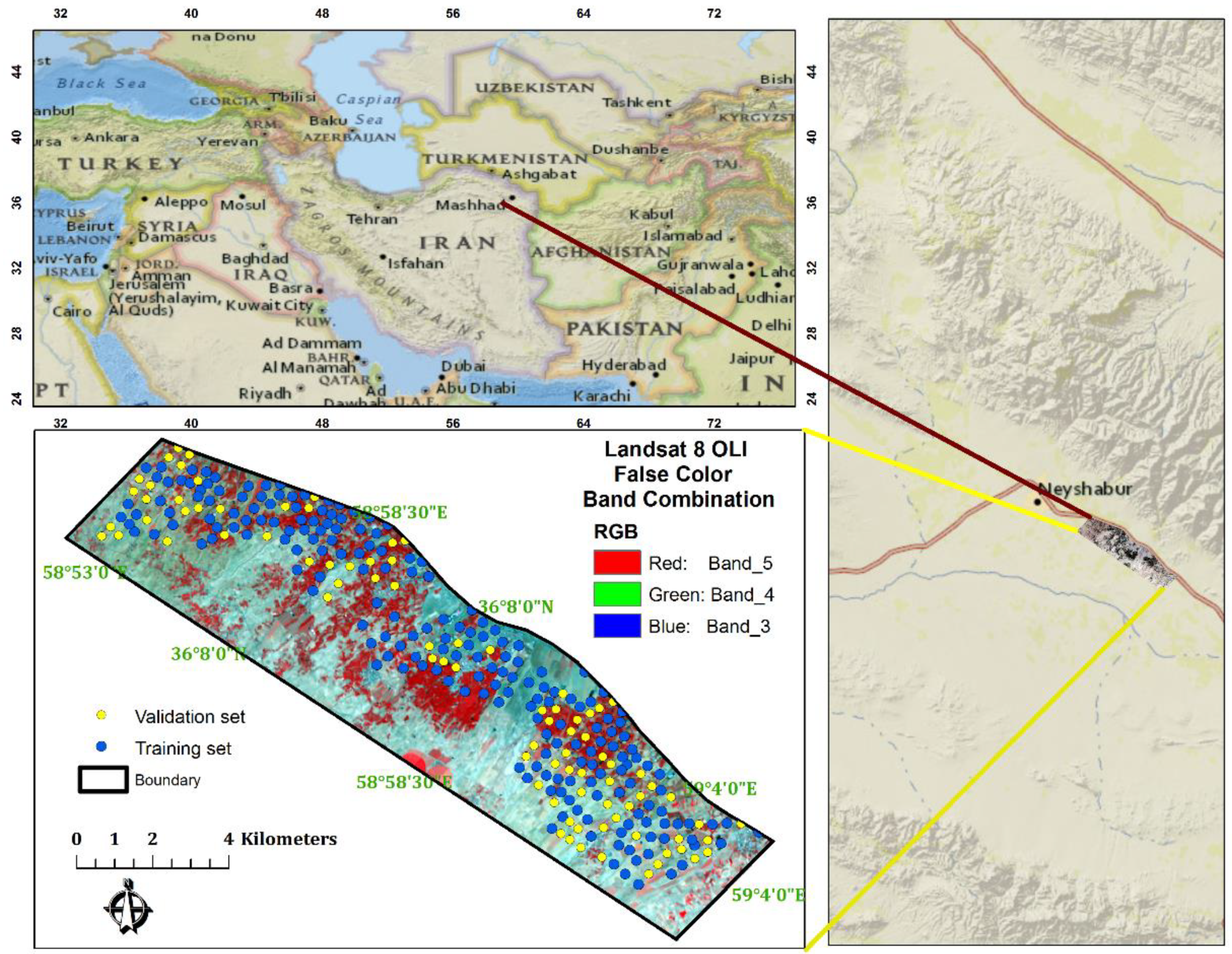
2.1. Study Area

The study area (~100 km²) is located within the Neyshabur plain of the Khorasan-e-Razavi province, Northeast Iran (Figure 1). It is bounded by latitudes 36°02′ N and 36°08′ N, and longitudes 58°53′ E and 59°04′ E. The climate is semi-arid, with a mean annual air temperature of 14.5 °C and mean annual precipitation of 233.7 mm. The Neyshabur plain stretches from NW to SE direction and Aridisols and Entisols are the major soil types [53,54].

2.2. Soil Sampling and Analysis

Based on a grid-stratified sampling scheme, a total of 288 locations for the collection of soil samples (0–20 cm depth, by soil auger) were considered, and triplicate composite samples were collected for each point. Sample coordinates were acquired with a portable global positioning system (GPS) (handheld Garmin eTrex^®H GPS) device. Soil samples were air-dried, pulverized, and sieved through 2 mm mesh. The Walkley–Black wet oxidation method [55] was used to determine SOC content (%). Soil available P (ppm or mg kg⁻¹) was determined using the Olsen method with a spectrophotometer [56].

2.3. Covariates Used for DSM

In this study, topographic variables were derived from the digital elevation model (DEM) that can represent topography; soil and vegetation-based indices were generated from remote sensing data obtained from Landsat 8 OLI and Sentinel 2A MSI to represent organisms and parent material [57]; climate variables were obtained from “WorldClim” data set [58], and, based on some soil properties in the study area, four different sources of environmental covariates were used that could digitally represent soil formation factors. The digital soil mapping approach is based on the SCORPAN concept (soil, climate, organisms, topography, parent material, and spatial location) [59]. The covariate production process was performed using the ArcGIS 10.8 [60].

2.3.1. Remote Sensing-Based Indices

Landsat 8 OLI sensor, Collection 2 Level 2 Science Product, 160 path, 35 Row, Collection 2 level, satellite images from 4 different periods (2018–2021) were used. The specialized software of Land Surface Reflectance Code (LaSRC) was used to produce the Landsat 8 Surface Reflectance (SR) Science Products [61]. Additionally, Collection 2 Landsat Level-2 surface reflectance needs to be multiplied by a scale factor before using (SR = 0.0000275). In addition to Landsat-8, Sentinel-2 data have been used. Sentinel 2A MSI sensor, Level 2A Bottom of Atmosphere, R020 orbit number; defining the “Track”, T40SFF ID of the area, that has been visualized defining the “Granule”, and satellite images from 3 different years were used throughout recently years [37]. The spectral bands of the used sensors are given in

Table 1. Corresponding Landsat-8 and Sentinel-2 bands and characteristics.

Landsat-8 OLI			Sentinel-2A
Bands	Pixel Size (m)	Wavelength (µm)	Bands	Pixel Size (m)	Wavelength (nm)
B1-Coastal	30	0.435–0.451	B1-Coastal	60	443.9
B2-Blue	30	0.452–0.512	B2-Blue	10	496.6
B3-Green	30	0.533–0.590	B3-Green	10	560.0
B4-Red	30	0.636–0.673	B4-Red	10	664.5
B5-NIR *	30	0.851–0.879	B5-Vegetation Red Edge	20	703.9
B6-SWIR * 1	30	1.566–1.651	B6-Vegetation Red Edge	20	740.2
B7-SWIR * 2	30	2.107–2.294	B7-Vegetation Red Edge	20	782.5
B8-Pan	15	0.500–0.680	B8-NIR *	10	835.1
			B8A-Narrow NIR *	20	864.8
B9-Cirrus	30	1.36–1.38	B9-Water Vapor	60	945.0
B10-TIRS * 1	100	10.60–11.19	B10-SWIR *-Cirrus	60	1360.0
B11-TIRS * 2	100	11.50–12.51	B11-SWIR*	20	1613.7
			B12-SWIR*	20	2202.4

* Abbreviations: NIR: Near Infrared; SWIR: Short-Wave Infrared; TIRS: Thermal Infrared Sensor.

. Product information of satellite images used in the study is given in Supplementary Materials Table S1.

2.3.2. Topographic Derivatives

Generally, the effect of topography as defined by elevation, slope, and landscape location on SOC and soil Ava-P variation is well-recognized [30,62,63,64]. The topographic features of the study area were derived for a DEM (https://search.asf.alaska.edu/, accessed on 5 September 2021) [65]. Following Hengl and Reuter [66], terrain attributes of elevation (m), profile curvature, slope (%), flow accumulation, planform curvature, stream power index, and topographic wetness index were derived from the DEM and used as predictive-independent variables in the modeling (Table 2, Supplementary Materials Figure S1).

2.3.3. Climate Based Covariates

Climatic conditions, i.e., temperature and precipitation and their seasonal distributions, are critical drivers of SOC storage globally and at regional scales that affect both C input to soil and SOC decomposition [67]. In this context, the variables reported in Table 2 from the “WorldClim 2” dataset, a globally accessible open climate dataset, even in a small area, were used in our study [58] (Table 2, Supplementary Materials Figure S1).

2.3.4. Soil-Based Covariates

The amounts of SOC and soil Ava-P that we are aiming to predict tend to be related to the physical and chemical properties of the existing soil [17,67]. Generally, there is evidence of a global dependence of SOC storage capacity on fine fraction content, but this relationship is strongly dependent on climatic conditions, land use, clay type, and fine fraction size limits [67]. In our case, organic carbon additions may occur depending on the management practices in the agricultural piedmont plain, where irrigated farming activities are also carried out due to the arid climate. Thus, SOC may be affected from the soil texture. Raster maps produced with ordinary kriging (OK), which is the most basic geostatistics approach for clay, sand, and pH, were used as environmental variables (Table 2; Supplementary Materials Figure S1).

Table 2. Covariates used in this study.

Auxiliary Variables	Environmental Covariates
Digital Elevation Model (DEM)	Elevation (m)
	Slope (%)
	Profile curvature
	Planform curvature
	Topographic wetness index (TWI)
	Flow Accumulation
	Stream Power Index (SPI)
Remote Sensing Data (Both Landsat 8 OLI and Sentinel 2A MSI) (RS)	Topsoil grain size index [68]
	Saturation index [69]
	Normalized clay index [12]
	Normalized difference vegetation index (NDVI) [70]
	Green Normalized Difference Vegetation Index [GNDVI) [71]
Climatic Variables (CL)	BIO-1-Mean Annual Temperature (MAT) (°C)
	BIO-12-Annual Precipitation (mm)
	BIO-15-Precipitation Seasonality (CV)
	Total Solar Radiation (kJ m−2 year−1)
Soil Attributes (S)	Clay map produced with Ordinary Kriging (%)
	Sand map produced with Ordinary Kriging (%)
	pH map produced with Ordinary Kriging

Table 2. Covariates used in this study.

Auxiliary Variables	Environmental Covariates
Digital Elevation Model (DEM)	Elevation (m)
	Slope (%)
	Profile curvature
	Planform curvature
	Topographic wetness index (TWI)
	Flow Accumulation
	Stream Power Index (SPI)
Remote Sensing Data (Both Landsat 8 OLI and Sentinel 2A MSI) (RS)	Topsoil grain size index [68]
	Saturation index [69]
	Normalized clay index [12]
	Normalized difference vegetation index (NDVI) [70]
	Green Normalized Difference Vegetation Index [GNDVI) [71]
Climatic Variables (CL)	BIO-1-Mean Annual Temperature (MAT) (°C)
	BIO-12-Annual Precipitation (mm)
	BIO-15-Precipitation Seasonality (CV)
	Total Solar Radiation (kJ m−2 year−1)
Soil Attributes (S)	Clay map produced with Ordinary Kriging (%)
	Sand map produced with Ordinary Kriging (%)
	pH map produced with Ordinary Kriging

2.3.5. Selection of Environmental Covariates

In the study, environmental variables are given to represent soil formation factors digitally (Table 2; Supplementary Materials Figure S1). All covariates used in this study were aligned to the same grid cell resolution and extent. Here, a 30 m grid was used, and the alignment of grids was performed using nearest neighbor resampling where needed. The coordinate reference system used in this study was WGS 1984 UTM zone 40N (EPSG:32640). Twenty-four environmental variables were merged into singe dataset. From the stack layer, environmental variable values of 288 soil sampling locations were extracted. These operations were performed using the R “raster” package [72]. Variable selection with recursive feature elimination [73] was applied before the spatial predictive model was established for SOC and Ava-P on the 24 variables. The appropriate number of predictors for each soil feature and the final list of selected estimators are determined [23].

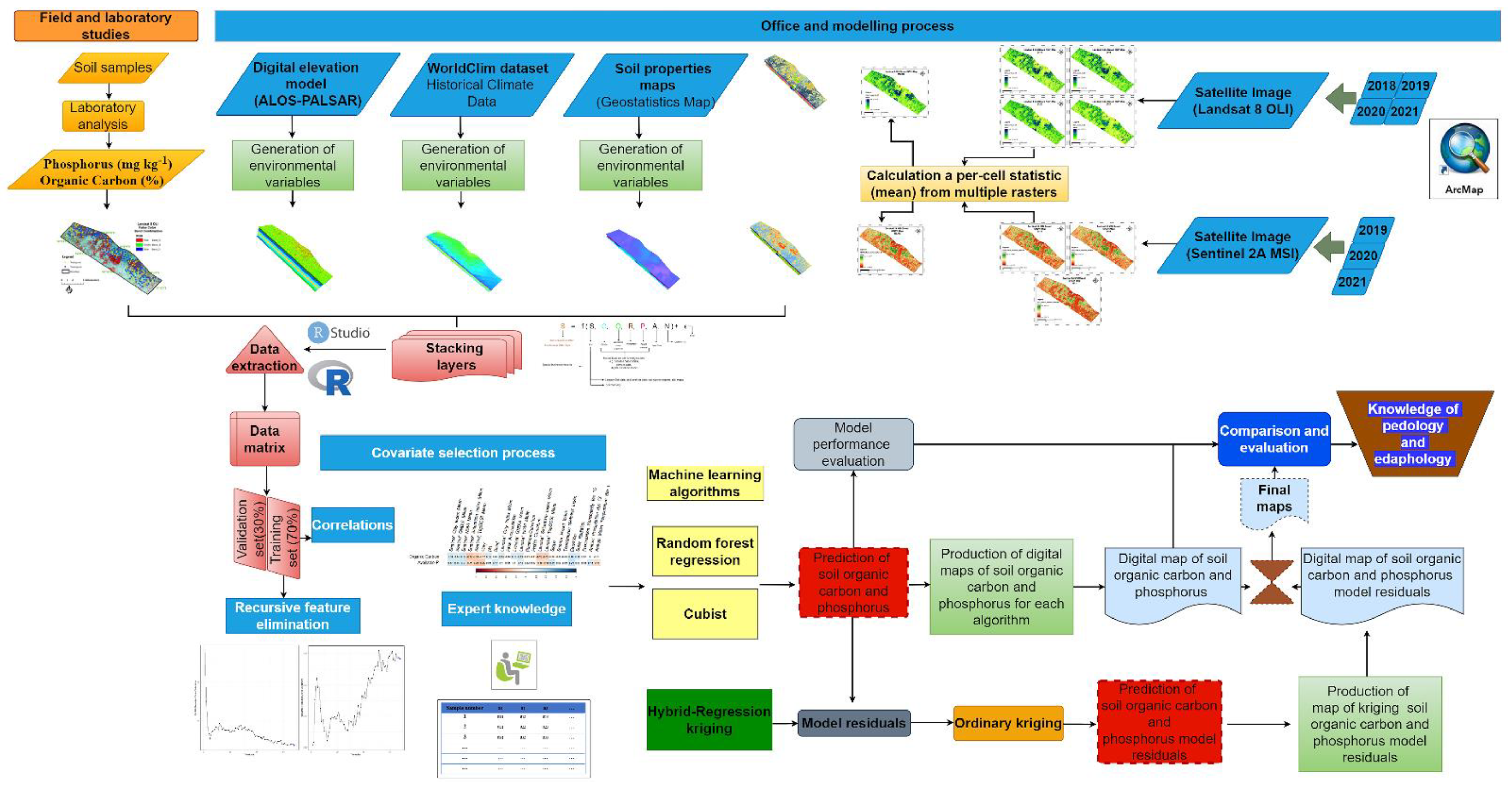
2.4. Modeling Process

Figure 2 presents the flowchart explaining the whole process. First, the “randomForest” [74], and the “cubist” [75] packages of the R software [76] were used to predict the SOC and Ava-P by regression model procedures. The sampled dataset was split into 70% for training (n = 201) and 30% for validation (n = 87), where the random sampling was fixed. In the parameter tuning process, the “mtry” parameter of the random forest model and the “committees” and “neighbors” parameter for regression were initially determined based on the repeated k fold cross-validation (n:5, repeated:3) [26].

2.5. Spatial Prediction of Soil Organic Carbon and Available Phosphorus Using Machine Learning Algorithms

The SOC and Ava-P content were modeled by Cubist, random forest, and regression kriging (hybrid model), which are explained in the following sections.

2.5.1. Cubist Algorithm

Cubist, also known as the piecewise linear decision tree approach, is based on the M5 algorithm [77,78,79]. In the Cubist model, sections are defined by a list of rules organized in a hierarchy. Cubist is a rule-based algorithm that has recently become increasingly used in the framework of digital soil mapping [1,24,29,80,81,82]. The approach used to grow trees in Cubist is similar to that used in classical regression tree models, such as classification and regression trees (CART). However, unlike CART, terminal tree leaves contain linear regression models instead of discrete class labels [83]. In Cubist, regression trees are reduced to a set of understandable rules where each rule is based on some condition, so that different linear models can capture local linearity in the predictive feature space. We performed Cubist modeling of SOC and Ava-P using the “Cubist” package in the R environment [75]. The cubist creates a clear model and provides the relative importance of estimators for interpretation [80].

2.5.2. Random Forest Algorithm

The random forest algorithm—developed by Breiman [84]—has been used very often as a regression method for estimating soil properties in digital soil mapping studies [85]. The approach of combining several random decision trees and their estimates with averages is preferred in digital soil mapping, because it is versatile enough to be applied to large-scale studies and provides information on the importance of the variables [42]. The detection of out-of-bag (OOB) errors for assessing the variable importance was conducted using 36.8% of the training dataset. The random forest algorithm requires 3 parameters: (i) mtry, the number of variables to be selected randomly at a node split having a default value of one-third of the total number of variables for regression, (ii) the number of trees parameter “ntree” with a default value of 500, and (iii) the size of the terminal node parameter “nodesize”, with a standard value of 5 for regression [86]. For each model, the importance of the environmental variables was determined using the “importance” function of the “randomForest” package [74], obtaining importance values for regression. The importance of each variable is the change in the OOB error when it is removed from the set of the environmental variables, noting that the larger the increase in the OOB error the higher the importance of the variable. The software computes two important measures of %IncMSE (increase in mean standard error) and IncNodePurity. %IncMSE is calculated for each tree with and without the relevant predictors. The mean value of the difference between the with and without cases for all the trees is then normalized to the standard deviation of the differences. In the published literature, the percentage increase in mean square error (%IncMSE) is the most used [87]. Top ranks in the variable importance graph indicate important common variables. To interpret the relative importance, the percentage increase in mean square error is between 0 to 100 [87,88,89].

2.5.3. Spatial Prediction of Soil Organic Carbon and Available Phosphorus with Hybrid Methods

Regression kriging (RK) is a hybrid spatial method that optimizes the prediction of soil properties at unsampled locations [90]. In the hybrid (RF–regression kriging and Cubist–regression kriging) approach of this study, the explanatory variation was estimated by RF and Cubist algorithms, and the process was carried out by summing the regression value of soil organic carbon and phosphorus and the kriging values of model residuals in non-sampled locations. By adding residual kriging to the maps created by the models, maps of soil organic carbon and available phosphorus content estimated by Cubist–kriging and random forest–kriging were produced, and model performance evaluation criteria were calculated in the validation datasets. In general terms, the mathematical equation specific to the study can be expressed as [33]:

$$Z_{RK-RF,Cubist}=Z_{RF,Cubist}\left(OC,P\right)+Z_{Ordinary Kriging}\left(OC,P\right)$$

(1)

where Z_{RK-RF, Cubist} is the soil organic carbon and available phosphorus value predicted by RK–(RF and Cubist), Z_RF, _Cubist (OC, P) is the soil organic carbon, and available phosphorus value by random forest (RF) and Cubist, and Z_{Ordinary Kriging} (OC, P) is the kriged residuals of random forest and Cubist models.

The first part of the equation is called the deterministic component, and the second part is called the stochastic. This distinction is important because it allows for decoupled interpretation of the two components and the use of different regression techniques [90] or different statistical methods (random forest, cubist, etc.) allows it to be implemented together.

2.6. Model Accuracy of Regression-Based Algorithms

The following criteria were used when evaluating the prediction performance in training and validation datasets for random forest, cubist, and hybrid model.

Root Mean Square Error

$$RMSE=\sqrt{\frac{{\sum }_{i=1}^n{\left(\mathrm{O}i-\mathrm{P}i\right)}^2}{n}}$$

(2)

Normalized root mean square error (NRMSE) as an absolute value between predicted and observed values using different types of normalization methods [91].

$$NRMSE=100\times \left(\frac{RMSE}{Normconstant}\right)$$

(3)

NRMSE values were determined with the “nrmse” function in the “hydroGOF” package in the R Core Environment program. The “Normconstant” criterion in this function is the standard deviation of the observations by default [92].

Mean absolute percentage error (MAPE), the average deviation of the predicted value from the observed value in percent [93].

$$MAPE=\frac{1}{n}{{\displaystyle \sum }}_{i=1}^n\frac{\left|\mathrm{O}i-\mathrm{P}i\right|}{\mathrm{O}i}$$

(4)

where Oi and Pi are the observed and predicted values, and n is the sample size.

Lin’s concordance correlation coefficient (LCCC) [94] measures the strength of the agreement between the observed and predicted values given as:

$$LCCC=\frac{2{\rho \sigma }_{obs}{\sigma }_{pred}}{{\sigma }^2{}_{obs}+{\sigma }^2{}_{pred}+{\left({\mu }_{obs}-{\mu }_{pred}\right)}^2}$$

(5)

where μobs and σobs are the mean and variance of the observed SOC and Ava-P value, μpred and σpred the corresponding values of the predicted values, and ρ is the correlation coefficient between the observed and predicted SOC and Ava-P value.

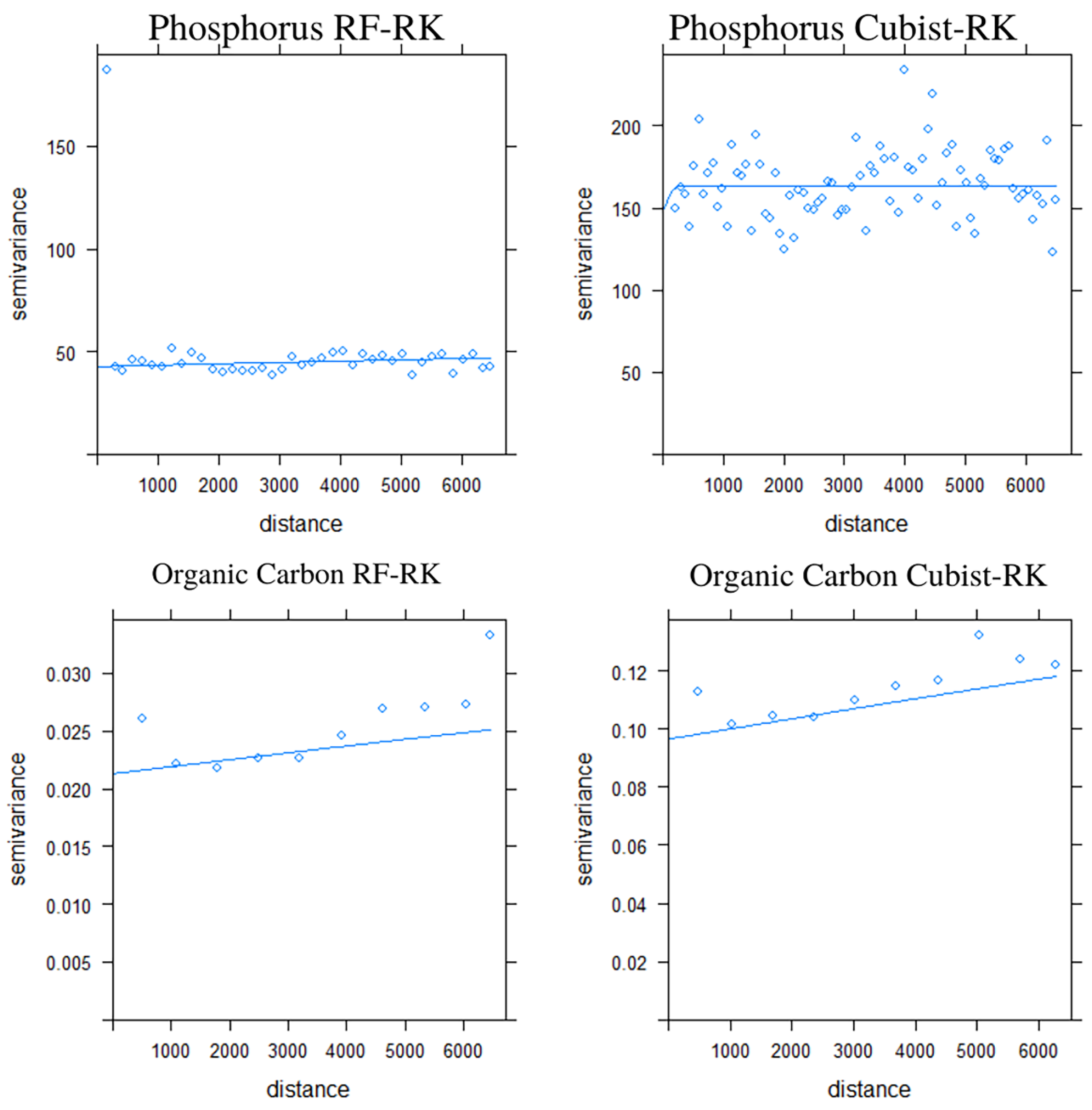
2.7. Analysis of Spatial Autocorrelation of Model Residuals

The residuals are considered errors and represent the component of a model that cannot be explained by the deterministic component [47]. Ideally, the residuals of a linear model should be independently and normally distributed. In Supplementary Materials Figure S4, each model residuals distributions results [76] were calculated using the “hist”, “qqnorm”, and “qqline” functions in the R Core Environment. Because normality is not a prerequisite for geostatistical analysis, model residuals were processed and analyzed without transformation [95]. Nugget, sill, and range values were obtained by using ArcGIS 10.8-Geostatistical Wizard-Ordinary Kriging tool for the model residuals of the samples with coordinates in the training set. Using these values, the semi variogram model and graphics were produced through the “gstat” [96,97] package in the R Core Environment program. The spatial variation structure, the Semi variogram, is determined using the following equation:

$$\gamma \left(h\right)=\frac{1}{2n\left(h\right)}{\displaystyle \sum }_{n=1}^n{[Z(X_i)-Z\left(X_i+h\right)]}^2$$

(6)

where n is the number of pairs of the sample separated by the distance h and Z_(Xi) the value of sampled point in ith point (i = 1, 2, 3, …, n).

To estimate model residuals at unsampled points,

$$Z\left(\mu \right)={\displaystyle \sum }_{i=1}^n{\lambda }_{i}Z({\mu }_i)$$

(7)

where Z_(μ) is the predicted value of unsampled point; Z_(μi) is the ith point measured value; λ_i is the ith point by undefined weight for the estimated value; n is the number of sampled values.

Moran’s Index is the traditional method for measuring autocorrelation, similar to Pearson’s correlation statistics for independent samples [98]. In both Moran’s Index and Pearson’s correlation, statistics range from +1.0 to −1, where +1 is a strong positive spatial autocorrelation, 0 a random pattern, and −1.0 a strong negative autocorrelation [99]. ArcGIS 10.8–Arctoolbox–Spatial Statistics toolbox–Analyzing Patterns was applied to the residuals of each model using the tool and Moran’s Index was calculated [60]. In addition, the relevant program outputs are given in Supplementary Materials Figure S2.

Moran’s Index (MI) is defined as:

$$MI=\left[\frac{n}{{\sum }_{i=1}^n{\sum }_{j=1}^n{w}_{ij}}\right]\left[\frac{{\sum }_{i=1}^n{\sum }_{j=1}^n{w}_{ij}\left(x_i-\overline{x}\right)\left(x_j-\overline{x}\right)}{{\sum }_{i=1}^n{\left(x_i-\overline{x}\right)}^2}\right]$$

(8)

where n is the number of points, x the variables of interest, $\overline{x}$ the mean of x, and W_ij the spatial weight describing the neighbor or distance between the ith and jth point.

3. Results and Discussion

3.1. Results of Descriptive Statistics

Descriptive statistics of soil properties are shown in

Table 3. Descriptive statistics of soil properties in the soil data set.

	Dataset	Count	Mean	SD *	CV *	Minimum	Median	Maximum	Skewness	Kurtosis
Available Phosphorus (mg kg−1)—Ava-P	Training	201	19.33	16.58	85.74	2.40	11.60	70.40	1.28	0.68
	Validation	87	17.36	15.36	88.47	2.40	10.40	70.40	1.60	2.08
Soil Organic Carbon (%)—SOC	Training	201	0.73	0.33	45.83	0.17	0.67	2.23	1.95	5.06
	Validation	87	0.73	0.31	42.96	0.25	0.67	1.83	1.38	2.14

* Abbreviations: SD: Standard deviation, CV: Coefficient of variation (%).

. The observed Ava-P content ranged from 2.40 to 70.40 mg kg⁻¹ with a mean of 19.33 mg kg⁻¹ and a CV of 85.74% in the training set; ranged from 2.40 to 70.40 mg kg⁻¹ with a mean of 17.36 mg kg⁻¹ and a CV of 88.47% in the validation data set. The observed SOC content ranged from 0.17 to 2.23% with a mean of 0.73% and a CV of 45.83% in the training data set; ranged from 0.25 to 1.83% with a mean of 0.73% and a CV of 42.96% in the validation data set. In the study area, both Ava-P and SOC presented a positively skewed distribution due to the heterogeneous land use in the area. The coefficient of variation is greater than 36% in both data sets for phosphorus and soil organic carbon. Based on the CVs classification proposed by Wilding [100], SOC and Ava-P content have a high variability in the study area. The training and validation set of both soil properties are represented by good and comparable data distribution, given the similarities in the coefficients of variation (Table 3). Positive skewness implies that the majority of SOC and Ava-P values are clustered near the left tail of the distribution, with fewer values greater than the mean (Table 3; Supplement Material Figure S3), which may have an impact on the ML models’ performance. In this case, our data splitting procedure is appropriate to the modeling process [64]. Shahbazi et al. [31] reported that the spatial variability of phosphorus and organic carbon is high in a semi-arid area of Iran where agricultural production is intense and there are different land uses.

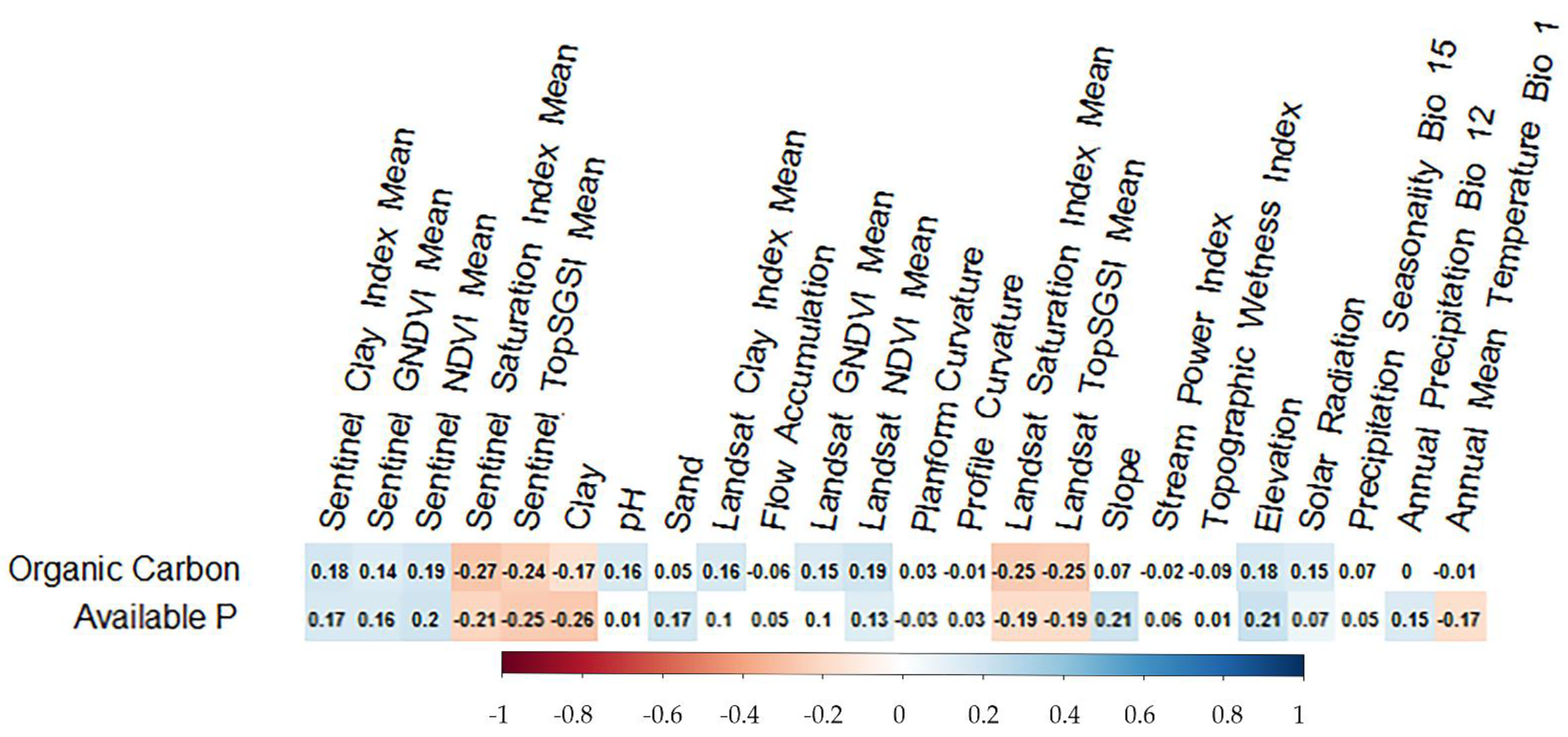
3.2. Selection of Covariates and Correlation Results

As a result of the methodology followed in Section 2.3.5, predictors are ranked in relative order from most important to least important (Figure 3). In addition, Pearson correlation values between environmental variables and target soil properties were also considered [2]. In addition, expert knowledge [101] was added to the process of creating the environmental variable set, and the final predictive environmental variable set, the random forest algorithm, and those below 40% of the relative importance of the environmental covariates were removed from the models. [102,103]. Finally, the models were trained by the rest of the environmental covariates. The variables used in the final model for the two target soil properties and the attribute information in the training validation set are given in the Supplement Material Table S2.

In our study area, significant statistical Pearson correlation values were found between soil organic carbon and available phosphorus and Clay, Sand, and pH (Figure 4). Although there was a negative correlation between SOC and Clay specific of our region, clay has a role to protect organic matter, and SOC can increase linearly with clay content on a regional and global scale [67,104]. The negative correlation between clay and SOC in our study area (Figure 4) can be explained by the fact that where SOC decomposition and storage are limited by other factors (e.g., annual precipitation), clay may not be that important for SOC stabilization [1]. Available P (Ava-P) correlated positively with elevation (r = 0.21) and Sentinel NDVI (r = 0.20), but negatively with clay (r = −0.26) and Landsat TopSGSI (r = −0.19) and Sentinel TopSGSI (r = −0.25). Conversely, Ava-P showed negative correlations with Landsat Saturation Index and Sentinel Saturation Index and positive correlations with Sentinel GNDVI and Landsat NDVI; correlation coefficients ranged from −0.19 to 0.16 (Figure 4). On the other hand, soil organic carbon (SOC) correlated positively with elevation and negatively with Landsat Saturation Index, Sentinel Saturation Index, Landsat TopSGSI, and Sentinel TopSGSI. Generally, soil chemical properties are expected to show the strongest correlation with remote sensing data [23,105]. TWI and SPI did not show any significant correlation with soil properties in the study area. Solar radiation, one of the climate variables, showed a positive relationship with SOC. Ava-P showed a weak positive correlation with annual precipitation and a weak negative correlation with annual mean temperature. SOC did not show any correlation with rainfall and temperature in the study area, which may be related to the coarser spatial resolution of climate variables compared to the other environmental variables used. In addition, regional agricultural activities in the study area (e.g., irrigation) might have masked the effect of climate [67].

3.3. Performance of Regression Based Algorithms

Table 4. Comparisons of the accuracy of cubist and random forest models for calibration and validation dataset, additionally accuracy of hybrid models for the validation dataset.

Variable	Model	Training				Validation				Hybrid Model-Validation
		LCCC	RMSE	NRMSE	MAPE	LCCC	RMSE	NRMSE	MAPE	LCCC	RMSE	NRMSE	MAPE
Ava-P	Cubist	0.52	13.02	78.6	69.6	0.13	15.94	103.9	105.5	0.13	15.95	103.9	124.1
	RF	0.88	6.63	40.0	46.8	0.26	14.86	96.8	126.3	0.27	14.81	96.5	123.8
SOC	Cubist	0.06	0.33	99.4	30.8	0.16	0.30	94.2	30.4	0.21	0.28	91.5	32.01
	RF	0.84	0.15	45.2	15.4	0.19	0.30	94.5	33.6	0.20	0.30	94.8	33.68

Abbreviations: RF: Random Forest, Ava-P: Available Phosphorus, SOC: Soil Organic Carbon, NRMSE: Normalized root mean square error, RMSE: Root Mean Square Error, MAPE: Mean Absolute Percentage Error, LCCC: Lin’s Concordance Correlation Coefficient.

shows the values of the model performance criteria for the training and validation data set for Ava-P and SOC estimates. SOC showed the highest LCCC (0.19) in the random forest algorithm in the validation data set, while both models had the same RMSE (0.30%) for SOC. For validation data set, Ava-P had the highest LCCC (0.26) in the random forest algorithm, whereas the lowest RMSE (14.86 mg kg⁻¹) was obtained with the random forest algorithm. For the training dataset, the SOC showed the highest LCCC (0.84) in the random forest algorithm; however, the lowest RMSE (0.15%) for the SOC was obtained with the random forest model. Again, in the training dataset, Ava-P had the highest LCCC (0.88) in the random forest algorithm, and the lowest RMSE value was obtained again in the random forest algorithm.

The results showed that different algorithms have different SOC and Ava-P prediction capabilities at unsampled locations. Additionally, the difference in prediction accuracy for different algorithms may be related to the various mathematical functions of each algorithm [27]. Zeraatpisheh et al. [27] using different environmental variable sets, obtained LCCC values between 0.39 and 0.54 and RMSE values between 0.25 and 0.35 for RF and Cubist models, respectively, in their estimation of organic carbon in the southeast of Iran. When our results (Table 4) are considered, model performance criteria are close to each other with the results obtained in the relevant region, an alluvial area where agricultural activities are carried out and where different land uses are located, under similar climatic conditions. Shahbazi et al. [31], in a similar study area in the northwest of Iran, obtained an LCCC value of 0.71 in the training set with the Cubist algorithm and an LCCC value of 0.24 in the validation set. The literature results demonstrate that similar model results are obtained in arid and semi-arid environmental conditions of Iran. According to Maleki et al. [106], using the random forest algorithm, the value of RMSE was 0.36% in the surface samples in the estimation of soil organic carbon; considering that the dataset distribution of organic carbon [106] is very similar to our study, it can be stated that the lower RMSE values obtained in our study are due to the different environmental variables we added. The use of climate variables, which was available as open source in our study area, is probably limited by a relatively coarse spatial resolution compared to other environmental variables; thus, climate contributed relatively less to model results.

When the spatial maps of the obtained pure machine learning algorithms are examined, the algorithm-specific differences can be seen spatially. Accordingly, considering Table 4, the hybrid modeling process could not significantly improve the model performance. This situation has been widely studied in-depth and it has been determined that the spatial relationships of the model residuals for both algorithms and both soil properties are quite weak as a result of the random division of the training set in the modeling process. Ma et al. [1] reported that as a result of the integration of the model residuals of the Cubist algorithm with regression kriging in the northeast of China, the model performances improved, which was due to the spatial autocorrelation between the residuals. Pouladi et al. [24] compared RF and Cubist algorithms and hybrid approaches of these two algorithms for the estimation of soil organic carbon using remote sensing and topographic variables in their study, in an area with high organic matter content in the central regions of Denmark, which has relatively different climatic conditions compared with our study area. In their study, RMSE values of 4.20% and 3.99% were obtained for RF and Cubist for SOC, respectively. In the hybrid technique of both algorithms, 3.35% RMSE for RF-Kriging and 2.99% RMSE for Cubist–kriging were obtained. It has been reported that the improvement of model results requires a high-density sampling, which allows for spatial autocorrelation among model residuals. Guo et al. [21] compared the random forest and random forest–regression kriging methods for estimating soil organic matter in southern China and reported that if the spatial structure of the model residues is established, the random forest regression kriging approach can perform well in estimating and mapping soil organic matter. Sönmez et al. [107] used climate, topography, soil physical properties, parent material, geology, vegetation, and land use type information as environmental variables to estimate soil organic carbon content within the scope of establishing Türkiye’s national spatial soil organic carbon information system. They used the linear regression–regression kriging method and obtained a RMSE equal to 0.42%. Considering the similarity of the national study and environmental variables, the results obtained with the hybrid modeling technique were found close to the literature.

NRMSE values, which are based on the relationship between the RMSE values obtained in both approaches and the standard deviation of the observations, produced results similar to the RMSE and LCCC in the training and validation sets. The MAPE values, which allow us to judge the general acceptance of the obtained models, showed a value of about 30% as a result of modeling SOC with all methods. In this regard, these values indicate that estimates have a logical framework [92].

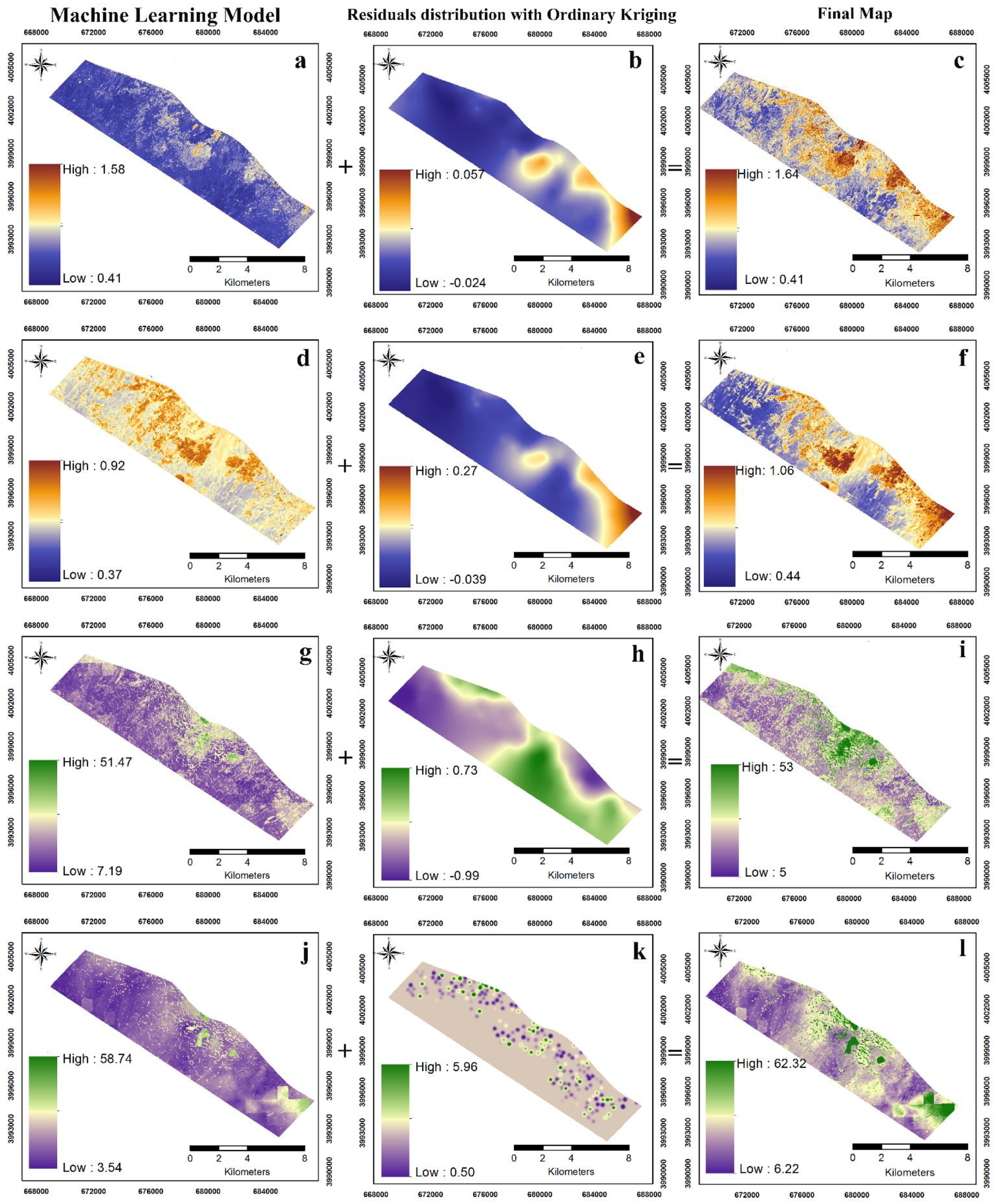
3.4. Spatial Prediction of Soil Organic Carbon and Available Phosphorus

3.4.1. Model Residuals of Soil Organic Carbon and Available Phosphorus

The degree of spatial correlation was determined by calculating the nugget/sill ratio of the semi variograms. A low nugget/sill ratio (i.e., lower than 25%) indicates a strong spatial correlation, a high ratio (i.e., higher than 75%) indicates a weak spatial correlation, and a median ratio (i.e., between 25% and 75%) means a moderate spatial dependency [108]. Fitted semi variogram parameters and Global Moran Index values of the calculated model residuals are given in

Table 5. Semi variogram model properties of model residuals for phosphorus and organic carbon using random forest and cubist models.

Variable	Model	Model	Nugget	Sill	Nugget/Sill Ratio	Effective Range (m)	Class of Spatial Structure	Moran’s Index
Residual Ava—P	Cubist-RK	Spherical	130.44	168.61	77.36	694	Weak	0.0380
	RF-RK	Exponential	40.75	46.34	87.93	1826	Weak	0.0325
Residual SOC	Cubist-RK	Spherical.	0.097	0.12	80.83	6208	Weak	0.043
	RF-RK	Spherical.	0.021	0.03	66.66	6589	Moderate	−0.022

Abbreviations: RF-RK: random forest combined with kriging, RK: Regression kriging, Ava-P: Available Phosphorus, SOC: Soil Organic Carbon.

. In Supplementary Materials Figure S2, reports of the Global Moran Index calculated with the ArcGIS 10.8–Spatial Statistics–Analyzing Pattern–Spatial Autocorrelation (Moran’s I) tool are given. The Global Moran’s Index values used as a spatial autocorrelation measure were also very close to 0 (Table 5). These values indicate that there is no autocorrelation among the residues and that there is a high degree of spatial randomness. Semi variogram parameters can be examined as well as Moran’s Index values can be used to determine the autocorrelation of model residuals before hybrid modeling [21].

Figure S4 in Supplementary Materials shows the histograms of the calculated model residuals (i.e., the observed SOC and Ava-P minus the deterministic model estimates). The data contain negative and positive values. No transformation was made to avoid compromising interpretability. For Ava-P resulting from both the RF and Cubist algorithms, the residual histogram shows a normal distribution that is suitable for the required normality assumption. For SOC, this assumption was not seen as appropriate due to the outliers in the model residues obtained as a result of the RF and Cubist algorithms [109].

In addition, we plotted the omnidirectional variograms of the residuals and the fitted semi variogram models in Figure 5. When the obtained semi variogram graphics are examined, it is evident that the model residuals do not show spatial correlation as reported in Figure 3d in [47]. All variograms models of the residuals had large nugget/sill ratios (Table 5) that is the most common result of digital soil mapping analyses when dealing with sparse soil observation sets [47,109,110]. These results are not rare in digital soil mapping. Szatmári and Pásztor [110] conducted the random forest–kriging process with spatially unrelated residues in the modeling process of soil organic carbon in their study across Hungary and obtained lower RMSE values compared to the compared models. Vaysse and Lagacherie [110] (Figure 3; second graph) found that the nugget/sill ratios of model residuals obtained as a result of random forest algorithm in the process of spatial modeling of soil organic carbon in the south of France were quite high, and reported that this resulted in underestimating the uncertainty in the forecasting process. Finally, these residuals were used for ordinary kriging [47], and the results were added to the RF and Cubist predictions (Figure 6).

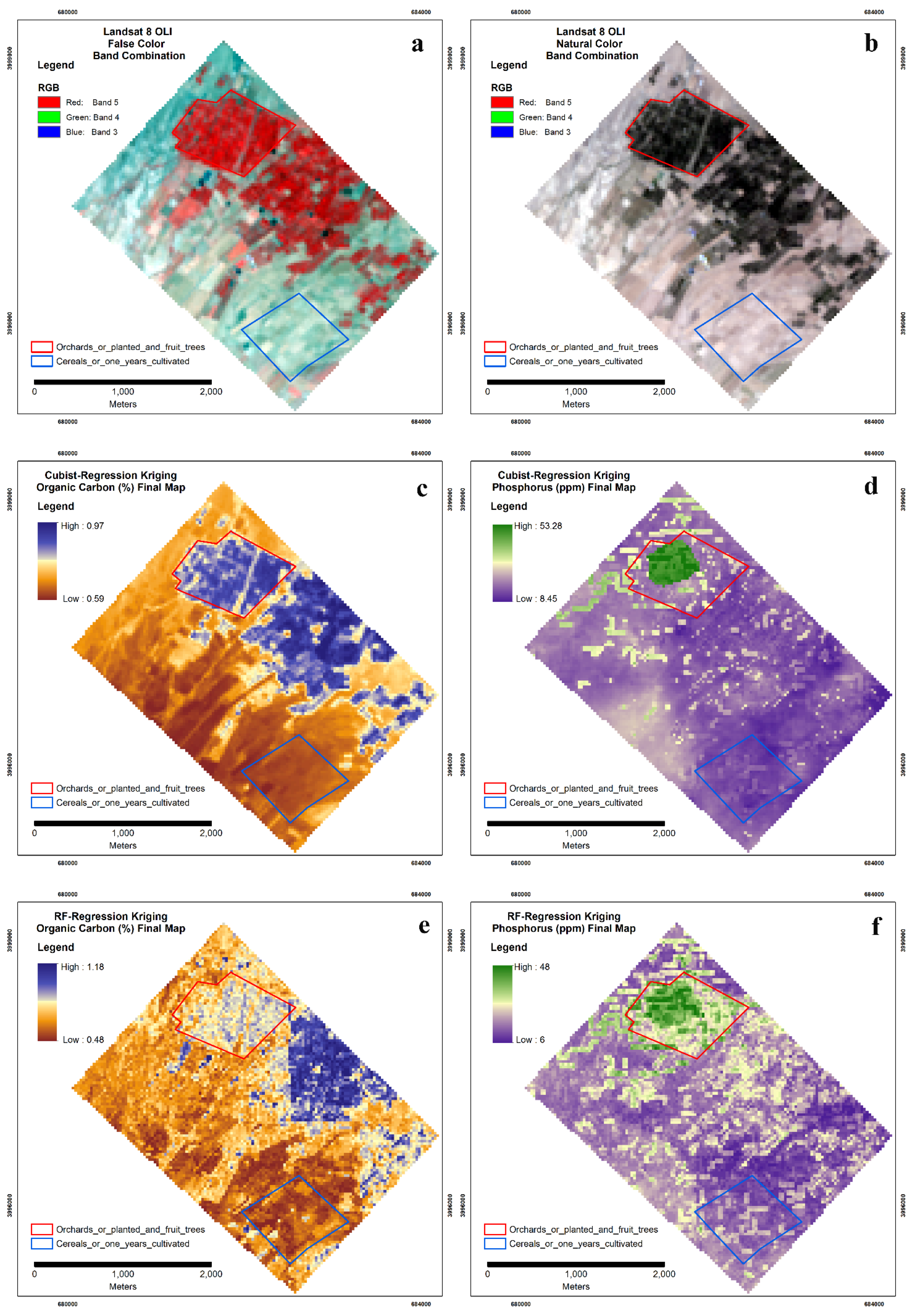
3.4.2. Spatial Prediction and Mapping

We estimated and mapped the spatial distribution of organic carbon and available phosphorus using hybrid techniques alongside RF and Cubist algorithms. Although the SOC varies greatly throughout the study area, a geographic orientational increase or decrease is not seen in digital maps produced by pure machine learning algorithms (Figure 6a,d). SOC was relatively low in the northwest of the study area, where low altitude and dry farmland under barley and wheat were present. However, in the middle regions of the study area, where orchards or fruits trees were found as a result of careful photo interpretation via Google earth, SOC was estimated relatively high by both algorithms. This is mainly due to land use type changes. Permanent vegetation farmland has a higher SOC than land with annual crops that are bare during some periods of the year and subject to more intensive tillage processes. Mayes et al. [111], examining the effects of land use on surface SOC in the Konya Basin, one of Türkiye’s important agricultural regions and where arid climatic conditions prevail, reported significant differences in SOC between annual crops and orchards. The increase in SOC in orchards may be due to agricultural practices such as manure management (fertilizer application), surface litter accumulation, tree canopy, and higher soil moisture, which enhance carbon sequestration [112]. Thus, SOC may tend to accumulate higher than on land where other annual crops are grown. Minor differences were found between CubistRK and RFRK in SOC spatial prediction maps in the study area (Figure 6c,f). As a result of the RK estimation of both models, the maximum SOC value increased in the study area. Generally, the extreme values of SOC may be underestimated in SOC estimations made with machine learning algorithms. Even though machine learning techniques are not sensitive to normal distributions compared to linear methods or kriging methods, the problem of sensitivity and extrapolation to the input data may persist, probably due to poor estimation of outliers and smoothing as they are insufficiently represented in the data [47]. As a result of both RF and Cubist algorithms, model residuals appear similar across the study area (Figure 6b,e). However, the difference between the residual values from the model is high. This may be due to the mathematical approaches based on the predictions of two different algorithms [27]. Considering the minimum and maximum values of both the training set and the validation set of the SOC (Table 3), it can be stated that the RF-RK SOC map is more effective for practical purposes. Although Ava-P varies greatly throughout the study area, it is highly predicted in the southeast and east of the study area (Figure 6c,g). The range for RF is 7.19–51.47 mg kg⁻¹, and for Cubist, the range is 3.54–58.74 mg kg⁻¹. Land management practices can further affect the phosphorus content of soil surfaces. It is important to note that fertilizer management and the addition of organic fertilizers containing phosphorus are the most important factors in increasing available phosphorus [112]. In the digital Ava-P maps produced as a result of both machine learning algorithms, high phosphorus contents were estimated in the small areas in the middle regions of the study area (Figure 6c,g). This situation may be caused by excessive phosphorus fertilization, which contributes significantly to the vegetative development of fruit trees. This is a result that is compatible with the realities of the field. The predicted maps of phosphorus content are also heavily influenced by processes such as land use and plant nutrition management [113]; thus, there are other important environmental factors such as fertilizer applications and land use [29,114,115,116,117].

The fact that the index average variables obtained from the Landsat and Sentinel satellites for different years, which we added to the environmental variable data set, provide preliminary information about the land use, helped us to understand this difference. As a result of the Cubist algorithm, it can be seen that the climate variable, which is especially effective in the forecast map of phosphorus, produces maps with a fixed pixel resolution (1 km × 1 km) of the environmental variable, depending on the mathematical basis of the algorithm (Figure 6j,l). This is because the Cubist algorithm establishes a linear equation for pixels that meet certain conditions and estimates the phosphorus as a result of this equation. Partial linearity in the modeling process caused the cubist algorithm to produce more unacceptable spatial digital maps. The maps obtained at the end of the hybrid modeling process showed that the available phosphorus was high in the orchard’s distribution throughout the study area compared to the rest of the study area (Figure 6i,l). In this study, we spatially discovered that the spatial distribution of Ava-P is affected by agricultural practices; thus, incorporating data on crop rotations in annual croplands into the modeling process can help improve Ava-P estimates to supports agricultural management.

Figure 6. Map of predicted soil organic carbon and soil available phosphorus (First column: (a) RF-SOC, (d) Cubist-SOC, (g) RF-Ava-P, (j) Cubist-Ava-P, purely machine learning used in produced maps; second column: (b) RF-SOC residuals, (e) Cubist-SOC, (h) RF-Ava-P residuals, (k) Cubist-Ava-P residuals, model residual maps produced using ordinary kriging; third column: (c) RFRK-SOC, (f) CubistRK-SOC, (i) RFRK-Ava-P, (l) CubistRK-Ava-P, Final maps). Abbreviations: RF: Random forest, SOC: Soil organic carbon, Ava-P: Available phosphorus, RFRK: random forest combined with kriging, CubistRK: Cubist combined with kriging.

Figure 6. Map of predicted soil organic carbon and soil available phosphorus (First column: (a) RF-SOC, (d) Cubist-SOC, (g) RF-Ava-P, (j) Cubist-Ava-P, purely machine learning used in produced maps; second column: (b) RF-SOC residuals, (e) Cubist-SOC, (h) RF-Ava-P residuals, (k) Cubist-Ava-P residuals, model residual maps produced using ordinary kriging; third column: (c) RFRK-SOC, (f) CubistRK-SOC, (i) RFRK-Ava-P, (l) CubistRK-Ava-P, Final maps). Abbreviations: RF: Random forest, SOC: Soil organic carbon, Ava-P: Available phosphorus, RFRK: random forest combined with kriging, CubistRK: Cubist combined with kriging.

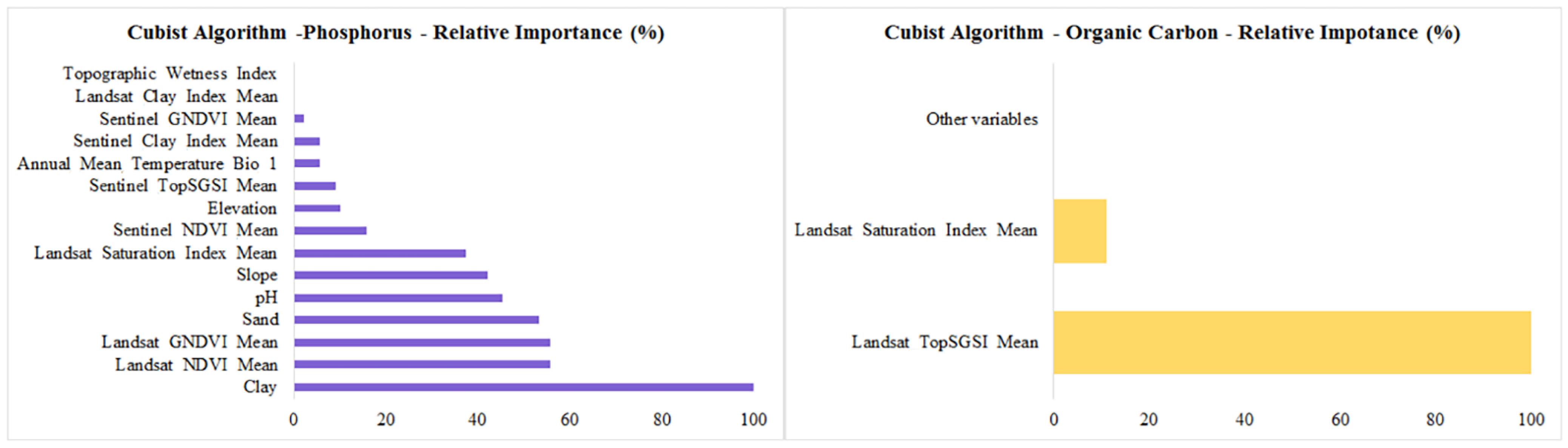
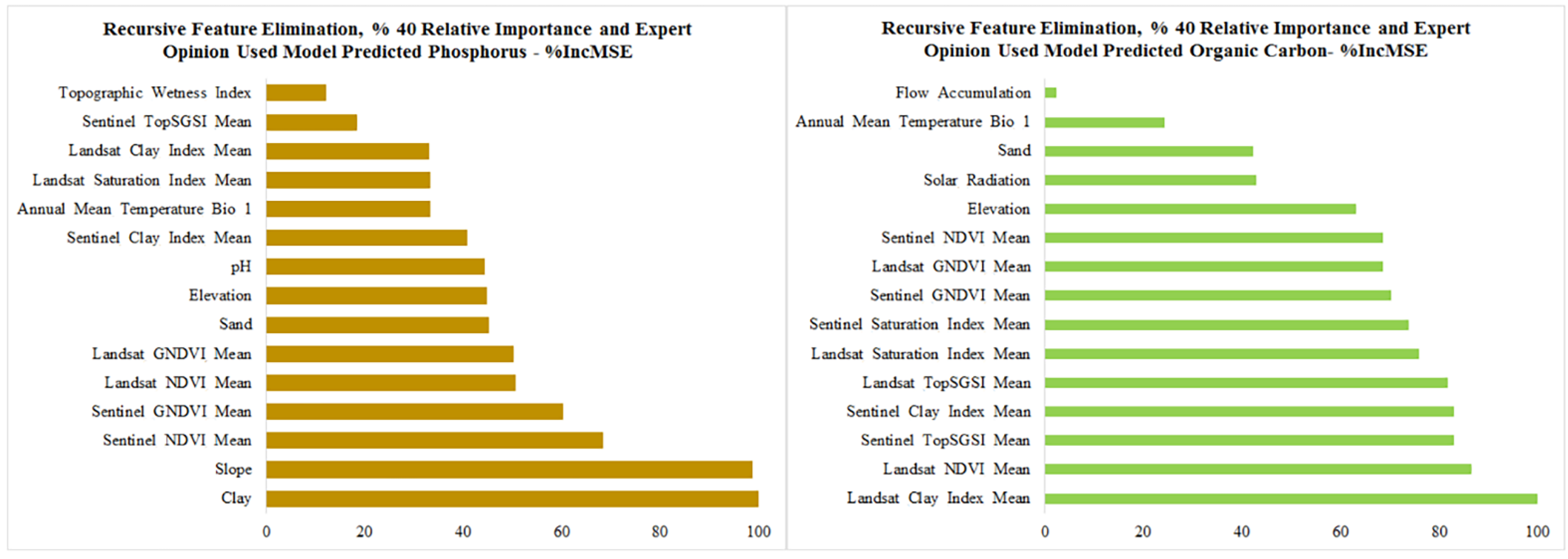
3.4.3. Importance of Environmental Covariates for Cubist and Random Forest

Figure 7 shows the contribution of environmental variables to the model in the estimation of soil properties of interest using the Cubist algorithm, as relative importance (%). Similarly, Figure 8 shows the contribution of environmental variables to the model in the estimation of soil properties of interest using the random forest algorithm, as relative importance (%). Clay was the most important environmental variable for Ava-P in both the Cubist and the random forest algorithms.

Clay, which is an important component of soil texture and is among the inherent soil properties, plays a very important role in nutrient availability while affecting various soil physicochemical properties [118]. For example, the SOC change is sensitive to many soil fundamental variables that were not considered to avoid too many input parameters in the modeling procedure, according to Gautam et al. [119]. SOC variability is also influenced by the inherent clay characteristics of the soil. Clay is also effective in the adsorption of phosphorus in different ways [120]. Indeed, the soil texture in these regions provides a basis for preparing precise soil maps [2,8]. In the framework of digital soil mapping, the effectiveness of the use of soil texture properties as an environmental variable is emphasized, especially in the estimation of dynamic soil properties [29,33,121]. The accuracy of soil organic carbon (SOC) mapping using images of the same periods of different years varies greatly due to weathering or atmospheric conditions in different years [122]. Luo et al. [123] report that statistical output rasters such as “Mean-Median” of time-series different index can provide better SOM estimation. However, the use of mean values in our study is aimed at increasing this estimation efficiency.

The effectiveness of remote-sensing-based index averages in modeling processes for both Ava-P and SOC is notable (Figure 7 and Figure 8). Regardless of spatial resolution, GNDVI and NDVI variables produced from Landsat and Sentinel satellites were the most important variables in the available phosphorus modeling. Taghizadeh-Mehrjardi et al. [124] reported the importance of NDVI and Soil Adjusted Vegetation Index (SAVI) variables in estimating soil SOC at a depth of 0–15 cm in different regions of Iran under similar climatic conditions. In this regard, the long-term average of these indices can give us preliminary information on land use. Indeed, Kunkel et al. [125] reported that SOC can be modeled with appreciable accuracy using only the NDVI and Enhanced Vegetation Index (EVI) from both MODIS and Landsat space platforms in the large basins of Eastern Australia. Remote-sensing-based environmental variables can improve the estimation of soil properties in arid and semi-arid areas, especially in areas where topographic variation is relatively low [126]. Emadi et al. [127] reported that rainfall is the most crucial feature driving the spatial variability of SOC contents, followed by the NDVI in the Mazandaran province of northern of Iran. Conversely, none of the climate variables in our environmental variable set were of relatively high importance in the modeling processes. The relatively low climatic variation of the existing area may have contributed to this situation. Indeed, “WorldClim” climate data, available as open source, represented the most important predictive variables in digital mapping of SOC at large scales where variation was sufficient [1]. The fact that few environmental variables are important in the modeling process of organic carbon with the Cubist algorithm is due to the mathematical basis of the Cubist algorithm in the modeling process. During the parameter optimization process, the value of “commites” was set at 20 and only Landsat TopSGSI and Landsat Saturation Index variables were used among the 20 rules created. This may be due to the two dominant land cover types in the study area when the images were taken. Indeed, Landsat TopSGSI and Landsat Saturation Index were included in the environmental variable dataset due to their widespread use in the literature on bare soil surfaces [9,68]. These two covariates have opposite pattern distributions in the field compared with the GNDVI and NDVI variables. Here, the Cubist algorithm did not indicate the relationships in the feature space in the data set with organic carbon.

3.5. Remarks Related to Land Management and Soil Properties

More intensively cultivated cropland or differences in permanent vegetation management practices affect the SOC distribution [128,129,130,131]. Wang et al. [132] have also shown that anthropogenic-related processes could impact SOC distribution in the agroecosystem. Qualitative assessment processes that consider land use by soil scientists can provide accurate insights into this issue. From a different perspective, the digital mapping accuracy of SOC can also be increased by using land-use history in arid areas with intensive agricultural activity [133]. In this study, we compared the maps produced by two different machine learning algorithms (RF and Cubist) and the Hybrid modeling process for SOC and Ava-P content in a semi-arid region of Iran. When the accuracy of the methods was evaluated, it was found that RF produced higher modeling accuracy and predictive maps suitable for the study area. We defined areas of interest (AOI) for two different land-use types in the southeast of the research region to examine the applicability of the SOC and Ava-P estimation to land use and to evaluate the estimation findings qualitatively. While determining these areas, we used the existing 4-year Landsat and 3-year Sentinel satellite images and considered our observations during soil sampling of the study area. Finally, we determined the areas by conducting a photo-interpretation process on the “historical images” in Google Earth^®. The comparison was made on the final maps obtained as a result of hybrid modeling (Figure 6c,f,i,l). The maps obtained as a result of overlaying the relevant areas on the soil properties maps estimated at the end of the Hybrid modeling process are given in Figure 9. False-color band combination and Natural color band combination maps obtained from Landsat satellite images during the years are given in Figure 9a,b, respectively. The most important point that attracts attention is that the maps produced with the RFRK methodology for organic carbon estimation and available phosphorus estimation can better reflect the variability within the areas of interest (AOI).

For the annual crop sub-area, the estimated SOC by the RFRK (Figure 9e) ranges from 0.48 to 1.18%. The SOC for the same area obtained with CubistRK (Figure 9c) is between 0.59 and 0.94%. For the orchard sub-area, the estimated Ava-P value by the RFRK (Figure 9f) ranges from 6 to 48 mg kg⁻¹. The Ava-P value obtained with CubistRK (Figure 9d) for the same area is between 8.45 and 53.28 mg kg⁻¹. There are six samples in the training and validation sets from the points sampled in the study area belonging to the “Cereals annually cultivated” fields. The average Ava-P content of these samples is 7.93 mg kg⁻¹ and the average SOC content of these samples is 0.53% (

Table 6. Available phosphorus and soil organic carbon contents of soil samples within the areas of interest (AOI).

	Cereals (Annually Cultivated)		Orchards or Planted and Fruit Trees
Count	6		7
Properties	Ava-P *	SOC *	Ava-P	SOC
Mean	7.93	0.53	35.94	0.86
SD *	1.67	0.08	20.25	0.48
CV * (%)	21.01	15.13	56.35	55.73
Minimum	5.6	0.46	15.6	0.25
Q1	6.5	0.46	16.8	0.46
Median	8	0.50	30.4	0.68
Q3	9.2	0.61	55.6	1.46
Maximum	10.4	0.64	70.4	1.46

* Ava-P: Available Phosphorus (mg kg⁻¹), SOC: Soil Organic Carbon (%), SD: Standard Deviation, CV (%): Coefficient of Variation.

). There are seven samples in the training and validation sets from the points sampled in the study area belonging to the “Orchards or planted and Fruit Trees” fields. The average Ava-P content of these samples is 35.94 mg kg⁻¹ and the average SOC content of these samples is 0.86% (Table 6). The Ava-P content obtained by RFRK was between 6.00 and 48.00 mg kg⁻¹, which was close to the range (5.6 to 70.40 mg kg⁻¹) of soil samples falling in the two regions (Table 6). Additionally, for lands with high or low vegetation, the spatial distribution characteristics of Ava-P estimated by RFRK are consistent with the real environment. The SOC obtained with RFRK ranged from 0.48 to 1.18%, which is close to the range (0.25 to 1.4%) of soil samples falling in the two regions. Additionally, the spatial distribution characteristics SOC estimated by RFRK are consistent with the real situation for lands with high or low vegetation. Both hybrid methodologies can spatially reflect the Ava-P and SOC differences between land uses. The maps produced with the RFRK methodology were found to be more effective in terms of reflecting the minimum values in both areas. For both RFRK and CubistRK, agricultural lands with perennial vegetation had a higher SOC than annual croplands, which will be more in line with the real situation. Similarly, Liu et al. [134] reported that their developed regression kriging-based hybrid approach was able to effectively map SOC with high spatial heterogeneity in their study area located southeast of the Jianghan Plain in China. Ava-P and SOC contents of the two dominant land use in our study area differed significantly from each other. This was also observed in other studies dealing with SOC estimation process with different DSM methodologies [135,136,137,138].

3.6. Limitations of the Case Study and Future Perspectives

Challenges that can be expected in associating existing soil data with digital soil formation factors in statistical space [139] were encountered in our case study. First, there was a shortage of well-distributed soil samples in the units we compared at the scale of land use in the study area. In our study, soil observations were taken according to the grid-stratified sampling scheme. When evaluated according to the current land uses, the number of samples in the “clustered” perennial planted agricultural areas in different regions of the study area could differ significantly compared to the annual cultivation areas. Second, another important limitation of this study is that long-term land use/land cover data were not included in the modeling process due to lack of reliable field data. Actually, the spatial distribution of the SOC and Ava-P contents of soils depends on factors such as climate and land morphology, but also land use. However, our study did consider land use in modeling but compared digital soil maps on a land-use scale, and the results indicated that soil organic carbon and available phosphorus can present very different values according to land use differentiation. Here, as a solution, studies should be conducted to compare the effectiveness of global land use/land cover data [140], which can be accessed as open source, in the modeling process [141]. However, the importance of obtaining information on land management or other land use-related variables in the form of “time series” should be emphasized [141]. Another limitation concerns the spatial resolutions of open-source multispectral satellite images. For precision agriculture applications, the areal size of the relevant soil feature represented in a pixel is important. In this case, it can be recommended that commercial PlanetScope satellites, which can offer open access to spatial and radiometrically higher resolution scientific studies that can better reflect heterogeneous phenomena in the area of interest, should be subject to studies [3]. In comparative studies, final DSM products are subject to numerous sources of erratic influences, including the mathematical variation of estimation algorithms [142]. Hengl et al. [47] stated that machine learning techniques do not depend on the assumption of a normal distribution but could potentially lead to the poor estimation of extreme values [4]. Additionally, the results of standard cross-validation will be significantly affected by outliers in areas with low sampling density, resulting in a pessimistic view of model accuracy. Therefore, more research should be undertaken on the selection and validation of training/test data in the modeling process in DSM studies with existing data [143]. In this study, it has been demonstrated that the spatial context of the residuals of the model in a randomly divided training set is important. Although solutions such as regression kriging will continue to be used in future studies, there is no significant improvement in spatial estimation in the absence of a spatial connection between model residuals.

Nowadays, with the growing abundance and improving resolution (spatial, temporal, and spectral), it may be suitable mapping soil SOC content via multispectral satellite data, as shown in previous research [3,4]. Remote sensing data to predict organic carbon [144], which is one of the most important factors affecting the leaching of crop protection products to groundwater, and phosphorus levels, which are critical in environmental interaction, together with arable land [144], in areas where the soil surface is constantly covered [131] may be useful to better represent spatial heterogeneity.

Nowadays, agricultural land management information may be more effective than natural factors in explaining SOC. Integrating cropping systems [145] into the modeling process can improve the SOC mapping of farmland in piedmont plains.

Our map comparison results, in which the soil scientist plays an active role, can be used to identify areas where concentrations are high and need to be protected, where uncertainty is high, and sampling is required for further monitoring [138].

It can be stated that sharing data sets obtained from different studies on open-source storage platforms can increase the sharing of information and help achieve more useful results, while increasing the possibilities of using model approaches.

4. Conclusions

With the integration of two different machine learning and hybrid methodologies, soil organic carbon and available phosphorus content maps of the topsoil in a piedmont plain with different land uses in north-eastern Iran were produced at a spatial resolution of 30 m. According to the validation set results, the random forest model was used to estimate the available phosphorus content, and the Cubist model was used to estimate the SOC, which provided more accurate verification statistics. Hybrid approaches to both soil features, on the other hand, reduced the uncertainty of spatial maps. Therefore, purely machine learning methods can be proposed for predictive mapping of SOC and Ava-P in similar areas and hybrid techniques that consider the spatial relationships of their model residuals. The main environmental variables in estimating SOC and Ava-P in this piedmont region were found to be key other soil properties and Landsat 8 OLI and Sentinel 2A MSI-based indices, which provide two different open-access spatial data. The effectiveness of the maps produced with different approaches, under two different dominant land uses, was evaluated in the study area in a way that allowed the soil scientist to make a qualitative assessment. The spatial distribution characteristics of Ava-P and SOC contents estimated by the hybrid approach are consistent with the real situation for lands under permanent vegetation or planted agriculture, as well as for annually cultivated areas. When comparing the assessed dominant land uses, orchard agricultural areas had the highest SOC (0.86%) and Ava-P (35.94 mg kg⁻¹) content compared to other land cover classes. The study area’s spatial distribution revealed that SOC was higher in orchards agricultural areas located in the central and eastern parts of the region. Digital maps depicting the spatial distribution of SOC and Ava-P and the forecast uncertainties can help prioritize activities for monitoring SOC and Ava-P levels in this area.

References

1. Ma, Y.; Minasny, B.; Wu, C. Mapping key soil properties to support agricultural production in Eastern China. Geoderma Reg. 2017, 10, 144–153. [Google Scholar] [CrossRef]
2. Naimi, S.; Ayoubi, S.; Demattê, J.A.M.; Zeraatpisheh, M.; Amorim, M.T.A.; Mello, F.A.O. Spatial prediction of soil surface properties in an arid region using synthetic soil image and machine learning. Geocarto Int. 2021; ahead-of-print. [Google Scholar] [CrossRef]
3. Žížala, D.; Minařík, R.; Zádorová, T. Soil Organic Carbon Mapping Using Multispectral Remote Sensing Data: Prediction Ability of Data with Different Spatial and Spectral Resolutions. Remote Sens. 2019, 11, 2947. [Google Scholar] [CrossRef]
4. Žížala, D.; Minařík, R.; Beitlerová, H.; Juřicová, A.; Skála, J.; Rojas, J.R.; Penížek, V.; Zádorová, T. High-resolution agriculture soil property maps from digital soil mapping methods, Czech Republic. Catena 2021, 212, 106024. [Google Scholar] [CrossRef]
5. Jenny, H. Factors of Soil Formation, a System of Quantitative Pedology; Dover Publications: New York, NY, USA, 1941. [Google Scholar]
6. Jenny, H.; Salem, A.E.; Wallis, J.R. Interplay of soil organic matter and soil fertility with state factors and soil properties. In “Study Week on Organic Matter and Soil Fertility”, Pontificiae Academiae Scientiarvm Scripta Varia; John Wiley & Sons: New York, NY, USA, 1968; Volume 32, pp. 5–36. [Google Scholar]
7. Yigini, Y.; Panagos, P. Assessment of soil organic carbon stocks under future climate and land cover changes in Europe. Sci. Total Environ. 2016, 557, 838–850. [Google Scholar] [CrossRef] [PubMed]
8. Rodrigo-Comino, J.; Senciales, J.M.; Cerdà, A.; Brevik, E.C. The multidisciplinary origin of soil geography: A review. Earth Sci. Rev. 2018, 177, 114–123. [Google Scholar] [CrossRef] [Green Version]
9. Mponela, P.; Snapp, S.; Villamor, G.; Tamene, L.; Le, Q.B.; Borgemeister, C. Digital soil mapping of nitrogen, phosphorus, potassium, organic carbon and their crop response thresholds in smallholder managed escarpments of Malawi. Appl. Geogr. 2020, 124, 102299. [Google Scholar] [CrossRef]
10. Ließ, M.; Gebauer, A.; Don, A. Machine Learning with GA Optimization to Model the Agricultural Soil-Landscape of Germany: An Approach Involving Soil Functional Types with Their Multivariate Parameter Distributions along the Depth Profile. Front. Environ. Sci. 2021, 9, 692959. [Google Scholar] [CrossRef]
11. Ma, Y.; Minasny, B.; Malone, B.P.; Mcbratney, A.B. Pedology and digital soil mapping (DSM). Eur. J. Soil Sci. 2019, 70, 216–235. [Google Scholar] [CrossRef]
12. Brown, K.S.; Libohova, Z.; Boettinger, J. Digital Soil Mapping. In Soil Survey Manual, USDA Handbook 18; Ditzler, C., Scheffe, K., Monger, H.C., Eds.; Government Printing Office: Washington, DC, USA, 2017; pp. 295–354. [Google Scholar]
13. FAO; ITPS. Soil Organic Carbon and Nitrogen: Reviewing the Challenges for Climate Change Mitigation and Adaptation in Agri-Food Systems. Rome, 2021, p. 3. Available online: https://www.fao.org/3/cb3965en/cb3965en.pdf (accessed on 15 January 2022).
14. Lal, R. Soil Organic Matter and Feeding the Future: Environmental and Agronomic Impacts, 1st ed.; CRC Press: Boca Raton, FL, USA, 2021. [Google Scholar] [CrossRef]
15. Nguyen, T.T. Predicting agricultural soil carbon using machine learning. Nat. Rev. Earth Environ. 2021, 2, 825. [Google Scholar] [CrossRef]
16. Kopittke, P.M.; Berhe, A.A.; Carrillo, Y.; Cavagnaro, T.R.; Chen, D.; Chen, Q.L.; Minasny, B. Ensuring planetary survival: The centrality of organic carbon in balancing the multifunctional nature of soils. Crit. Rev. Environ. Sci. Technol. 2022; ahead-of-print. [Google Scholar] [CrossRef]
17. Blume, H.P.; Brümmer, G.W.; Fleige, H.; Horn, R.; Kandeler, E.; Kögel-Knabner, I.; Wilke, B.M. Soil Organic Matter. In Scheffer/Schachtschabel Soil Science; Blume, H.P., Brümmer, G.W., Fleige, H., Horn, R., Kandeler, E., Kögel-Knabner, I., Wilke, B.M., Eds.; Springer: Berlin/Heidelberg, Germany, 2016. [Google Scholar] [CrossRef]
18. Winowiecki, L.A.; Bargués-Tobella, A.; Mukuralinda, A.; Mujawamariya, P.; Ntawuhiganayo, E.B.; Mugayi, A.B.; Vågen, T.-G. Assessing soil and land health across two landscapes in eastern Rwanda to inform restoration activities. Soil 2021, 7, 767–783. [Google Scholar] [CrossRef]
19. Wadoux, A.M.C.; Román-Dobarco, M.; McBratney, A.B. Perspectives on data-driven soil research. Eur. J. Soil Sci. 2021, 72, 1675–1689. [Google Scholar] [CrossRef]
20. Minasny, B.; McBratney, A.B.; Malone, B.P.; Wheeler, I. Digital Mapping of Soil Carbon. Adv. Agron. 2013, 118, 1–47. [Google Scholar] [CrossRef]
21. Guo, P.T.; Li, M.F.; Luo, W.; Tang, Q.F.; Liu, Z.W.; Lin, Z.M. Digital mapping of soil organic matter for rubber plantation at regional scale: An application of random forest plus residuals kriging approach. Geoderma 2015, 237, 49–59. [Google Scholar] [CrossRef]
22. Keshavarzi, A.; Sarmadian, F.; Omran, E.S.E.; Iqbal, M. A neural network model for estimating soil phosphorus using terrain analysis. Egypt. J. Remote Sens. Space Sci. 2015, 18, 127–135. [Google Scholar] [CrossRef] [Green Version]
23. Jeong, G.; Oeverdieck, H.; Park, S.J.; Huwe, B.; Ließ, M. Spatial soil nutrients prediction using three supervised learning methods for assessment of land potentials in complex terrain. Catena 2017, 154, 73–84. [Google Scholar] [CrossRef]
24. Pouladi, N.; Møller, A.B.; Tabatabai, S.; Greve, M.H. Mapping soil organic matter contents at field level with Cubist, Random Forest and kriging. Geoderma 2019, 342, 85–92. [Google Scholar] [CrossRef]
25. Wang, X.; Han, J.; Wang, X.; Yao, H.; Zhang, L. Estimating Soil Organic Matter Content Using Sentinel-2 Imagery by Machine Learning in Shanghai. IEEE Access 2021, 9, 78215–78225. [Google Scholar] [CrossRef]
26. Sakhaee, A.; Gebauer, A.; Ließ, M.; Don, A. Performance of three machine learning algorithms for predicting soil organic carbon in German agricultural soil. Soil Discuss. 2021; in review. [Google Scholar] [CrossRef]
27. Zeraatpisheh, M.; Garosi, Y.; Owliaie, H.R.; Ayoubi, S.; Taghizadeh-Mehrjardi, R.; Scholten, T.; Xu, M. Improving the spatial prediction of soil organic carbon using environmental covariates selection: A comparison of a group of environmental covariates. Catena 2022, 208, 105723. [Google Scholar] [CrossRef]
28. Sun, X.-L.; Lai, Y.-Q.; Ding, X.; Wu, Y.-J.; Wang, H.-L.; Wu, C. Variability of soil mapping accuracy with sample sizes, modelling methods and landform types in a regional case study. Catena 2022, 213, 106217. [Google Scholar] [CrossRef]
29. Matos-Moreira, M.; Lemercier, B.; Dupas, R.; Michot, D.; Viaud, V.; Akkal-Corfini, N.; Louis, B.; Gascuel-Odoux, C. High-resolution mapping of soil phosphorus concentration in agricultural landscapes with readily available or detailed survey data. Eur. J. Soil Sci. 2017, 68, 281–294. [Google Scholar] [CrossRef] [Green Version]
30. Adhikari, K.; Owens, P.R.; Ashworth, A.J.; Sauer, T.J.; Libohova, Z.; Richter, J.L.; Miller, D.M. Topographic controls on soil nutrient variations in a silvopasture system. Agrosyst. Geosci. Environ. 2018, 1, 180008. [Google Scholar] [CrossRef]
31. Shahbazi, F.; Hughes, P.; McBratney, A.B.; Minasny, B.; Malone, B.P. Evaluating the spatial and vertical distribution of agriculturally important nutrients—Nitrogen, phosphorous and boron—In North West Iran. Catena 2019, 173, 71–82. [Google Scholar] [CrossRef]
32. Zhou, T.; Geng, Y.; Ji, C.; Xu, X.; Wang, H.; Pan, J.; Lausch, A. Prediction of soil organic carbon and the C: N ratio on a national scale using machine learning and satellite data: A comparison between Sentinel-2, Sentinel-3 and Landsat-8 images. Sci. Total Environ. 2021, 755, 142661. [Google Scholar] [CrossRef]
33. Tziachris, P.; Aschonitis, V.; Chatzistathis, T.; Papadopoulou, M. Assessment of spatial hybrid methods for predicting soil organic matter using DEM derivatives and soil parameters. Catena 2019, 174, 206–216. [Google Scholar] [CrossRef]
34. Tziachris, P.; Aschonitis, V.; Chatzistathis, T.; Papadopoulou, M.; Doukas, I.J.D. Comparing Machine Learning Models and Hybrid Geostatistical Methods Using Environmental and Soil Covariates for Soil pH Prediction. ISPRS Int. J. Geo Inf. 2020, 9, 276. [Google Scholar] [CrossRef] [Green Version]
35. Fathololoumi, S.; Vaezi, A.R.; Alavipanah, S.K.; Ghorbani, A.; Saurette, D.; Biswas, A. Improved digital soil mapping with multitemporal remotely sensed satellite data fusion: A case study in Iran. Sci. Total Environ. 2020, 721, 137703. [Google Scholar] [CrossRef]
36. Burke, M.; Driscoll, A.; Lobell, D.B.; Ermon, S. Using satellite imagery to understand and promote sustainable development. Science 2021, 371, eabe8628. [Google Scholar] [CrossRef]
37. ESA. European Space Agency. Sentinel-2 User Handbook Rev 2. 2015. Available online: https://sentinels.copernicus.eu/documents/247904/685211/Sentinel7732_User_Handbook.pdf/8869acdf-fd84-43ec-ae8c-3e80a436a16c?t=1438278087000 (accessed on 15 November 2021).
38. Wulder, M.A.; Loveland, T.R.; Roy, D.P.; Crawford, C.J.; Masek, J.G.; Woodcock, C.E.; Zhu, Z. Current status of Landsat program, science, and applications. Remote Sens. Environ. 2019, 225, 127–147. [Google Scholar] [CrossRef]
39. Nguyen, T.T.; Pham, T.D.; Nguyen, C.T.; Delfos, J.; Archibald, R.; Dang, K.B.; Ngo, H.H. A novel intelligence approach based active and ensemble learning for agricultural soil organic carbon prediction using multispectral and SAR data fusion. Sci. Total Environ. 2022, 804, 150187. [Google Scholar] [CrossRef]
40. Shafizadeh-Moghadam, H.; Minaei, F.; Talebi-khiyavi, H.; Xu, T.; Homaee, M. Synergetic use of multi-temporal Sentinel-1, Sentinel-2, NDVI, and topographic factors for estimating soil organic carbon. Catena 2022, 212, 106077. [Google Scholar] [CrossRef]
41. Yuzugullu, O.; Lorenz, F.; Fröhlich, P.; Liebisch, F. Understanding Fields by Remote Sensing: Soil Zoning and Property Mapping. Remote Sens. 2020, 12, 1116. [Google Scholar] [CrossRef] [Green Version]
42. Hengl, T.; Miller, M.A.; Križan, J.; Shepherd, K.D.; Sila, A.; Kilibarda, M.; Crouch, J. African soil properties and nutrients mapped at 30 m spatial resolution using two-scale ensemble machine learning. Sci. Rep. 2021, 11, 6130. [Google Scholar] [CrossRef]
43. Silvero, N.E.Q.; Demattê, J.A.M.; Amorim, M.T.A.; dos Santos, N.V.; Rizzo, R.; Safanelli, J.L.; Bonfatti, B.R. Soil variability and quantification based on Sentinel-2 and Landsat-8 bare soil images: A comparison. Remote Sens. Environ. 2021, 252, 112117. [Google Scholar] [CrossRef]
44. Rosero-Vlasova, O.A.; Vlassova, L.; Pérez-Cabello, F.; Montorio, R.; Nadal-Romero, E. Modeling soil organic matter and texture from satellite data in areas affected by wildfires and cropland abandonment in Aragón, Northern Spain. J. Appl. Remote Sens. 2018, 12, 042803. [Google Scholar] [CrossRef]
45. Castaldi, F.; Hueni, A.; Chabrillat, S.; Ward, K.; Buttafuoco, G.; Bomans, B.; van Wesemael, B. Evaluating the capability of the Sentinel 2 data for soil organic carbon prediction in croplands. ISPRS J. Photogramm. Remote Sens. 2019, 147, 267–282. [Google Scholar] [CrossRef]
46. Kaya, F.; Başayiğit, L. Digital Mapping of Soil Organic Matter Using Open Source Accessible Products of ESA® in Arable Plain. ESA-ECMWF WORKSHOP Machine Learning for Earth System Observation and Prediction, ESA-ESRIN, 15 November 2021, Frascati. Available online: https://events.ecmwf.int/event/291/attachments/1518/2742/17._Kaya.pdf (accessed on 15 January 2022).
47. Hengl, T.; Nussbaum, M.; Wright, M.N.; Heuvelink, G.B.; Gräler, B. Random Forest as a generic framework for predictive modeling of spatial and spatio-temporal variables. PeerJ 2018, 6, e5518. [Google Scholar] [CrossRef] [Green Version]
48. Keskin, H.; Grunwald, S. Regression kriging as a workhorse in the digital soil mapper’s toolbox. Geoderma 2018, 326, 22–41. [Google Scholar] [CrossRef]
49. Song, Y.Q.; Yang, L.A.; Li, B.; Hu, Y.M.; Wang, A.L.; Zhou, W.; Liu, Y.L. Spatial prediction of soil organic matter using a hybrid geostatistical model of an extreme learning machine and ordinary kriging. Sustainability 2017, 9, 754. [Google Scholar] [CrossRef] [Green Version]
50. Fu, W.J.; Jiang, P.K.; Zhou, G.M.; Zhao, K.L. Using Moran’s I and GIS to study the spatial pattern of forest litter carbon density in a subtropical region of southeastern China. Biogeosciences 2014, 11, 2401–2409. [Google Scholar] [CrossRef] [Green Version]
51. Wadoux, A.M.J.-C.; McBratney, A.B. Hypotheses, machine learning and soil mapping. Geoderma 2021, 383, 114725. [Google Scholar] [CrossRef]
52. Zeraatpisheh, M.; Jafari, A.; Bagheri, B.M.; Ayoubi, S.; Taghizadeh-Mehrjardi, R.; Toomanian, N.; Xu, M. Conventional and digital soil mapping in Iran: Past, present, and future. Catena 2020, 188, 104424. [Google Scholar] [CrossRef]
53. Soil Survey Staff. Keys to Soil Taxonomy, 12th ed.; USDA-Natural Resources Conservation Service: Washington, DC, USA, 2014.
54. Bagherzadeh, A.; Ghadiri, E.; Darban, A.R.S.; Gholizadeh, A. Land suitability modeling by parametric-based neural networks and fuzzy methods for soybean production in a semi-arid region. Model. Earth Syst. Environ. 2016, 2, 104. [Google Scholar] [CrossRef] [Green Version]
55. Walkley, A.; Black, I.A. An examination of the Degtjareff method for determining soil organic matter, and a proposed modification of the chromic acid titration method. Soil Sci. 1934, 37, 29–38. [Google Scholar] [CrossRef]
56. Olsen, S.R.; Cole, C.V.; Watanabe, F.S.; Dean, L.A. Estimation of Available Phosphorus in Soils by Extraction with Sodium Bicarbonate; U.S. Govt. Print. Office: Washington, DC, USA, 1954.
57. Mulder, V.L.; De Bruin, S.; Schaepman, M.E.; Mayr, T.R. The use of remote sensing in soil and terrain mapping—A review. Geoderma 2011, 162, 1–19. [Google Scholar] [CrossRef]
58. Fick, S.E.; Hijmans, R.J. WorldClim 2: New 1km spatial resolution climate surfaces for global land areas. Int. J. Climatol. 2017, 37, 4302–4315. [Google Scholar] [CrossRef]
59. McBratney, A.B.; Santos, M.M.; Minasny, B. On digital soil mapping. Geoderma 2003, 117, 3–52. [Google Scholar] [CrossRef]
60. ESRI. ArcGIS User’s Guide. 2021. Available online: http://www.esri.com (accessed on 15 September 2021).
61. Sayler, K.; Zanter, K. Landsat 8 Collection 2 (C2) Level 2 Science Product (L2SP) Guide LSDS-1619 Version 2.0; EROS Sioux Falls: South Dakota, SD, USA, 2021. [Google Scholar]
62. Guo, Z.; Adhikari, K.; Chellasamy, M.; Greve, M.B.; Owens, P.R.; Greve, M.H. Selection of terrain attributes and its scale dependency on soil organic carbon prediction. Geoderma 2019, 340, 303–312. [Google Scholar] [CrossRef]
63. Adhikari, K.; Hartemink, A.E. Digital mapping of topsoil carbon content and changes in the driftless area of Wisconsin, USA. Soil Sci. Soc. Am. J. 2015, 79, 155–164. [Google Scholar] [CrossRef] [Green Version]
64. Adhikari, K.; Braden, I.S.; Owens, P.R.; Ashworth, A.J.; West, C. Relating topography and soil phosphorus distribution in litter-amended pastures in Arkansas. Agrosyst. Geosci. Environ. 2021, 4, e20207. [Google Scholar] [CrossRef]
65. ALOS PALSAR. Dataset: © JAXA/METI ALOS PALSAR L1.0 2007. ASF DAAC. Available online: https://asf.alaska.edu/ (accessed on 5 September 2021).
66. Hengl, T.; Reuter, H.I. Geomorphometry: Concepts, Software, Applications; Elsevier: Amsterdam, The Netherlands, 2008; Volume 33. [Google Scholar]
67. Wiesmeier, M.; Urbanski, L.; Hobley, E.; Lang, B.; von Lützow, M.; Marin-Spiotta, E.; Kögel-Knabner, I. Soil organic carbon storage as a key function of soils-A review of drivers and indicators at various scales. Geoderma 2019, 333, 149–162. [Google Scholar] [CrossRef]
68. Xiao, J.; Shen, Y.; Tateishi, R.; Bayaer, W. Development of topsoil grain size index for monitoring desertification in arid land using remote sensing. Int. J. Remote Sens. 2006, 27, 2411–2422. [Google Scholar] [CrossRef]
69. Hounkpatin, K.O.; Schmidt, K.; Stumpf, F.; Forkuor, G.; Behrens, T.; Scholten, T.; Amelung, W.; Welp, G. Predicting reference soil groups using legacy data: A data pruning and Random Forest approach for tropical environment (Dano catchment, Burkina Faso). Sci. Rep. 2018, 8, 9959. [Google Scholar] [CrossRef]
70. Tucker, C.J. Red and photographic infrared linear combinations for monitoring vegetation. Remote Sens. Environ. 1979, 8, 127–150. [Google Scholar] [CrossRef] [Green Version]
71. Gitelson, A.A.; Kaufman, Y.J.; Merzlyak, M.N. Use of a green channel in remote sensing of global vegetation from EOS-MODIS. Remote Sens. Environ. 1996, 58, 289–298. [Google Scholar] [CrossRef]
72. Hijmans, R.J. Raster: Geographic Data Analysis and Modeling. R Package Version 3.4-5. 2020. Available online: https://CRAN.R-project.org/package=raster (accessed on 15 November 2021).
73. Kuhn, M. Caret: Classification and Regression Training. R Package Version 6.0-86. 2020. Available online: https://CRAN.R-project.org/package=caret (accessed on 15 November 2021).
74. Liaw, A.; Wiener, M. Classification and regression by random Forest. R News 2002, 2, 18–22. [Google Scholar]
75. Kuhn, M.; Quinlan, R. Cubist: Rule- and Instance-Based Regression Modeling. R Package Version 0.2.3. 2020. Available online: https://CRAN.R-project.org/package=Cubist (accessed on 15 November 2021).
76. R Core Team. R: A Language and Environment for Statistical Computing; R Foundation for Statistical Computing: Vienna, Austria, 2021. [Google Scholar]
77. Quinlan, J.R. Learning with continuous classes. In Proceedings of the 5th Australian Joint Conference on Artificial Intelligence, Hobart, Tasmania, 16–18 November 1992. [Google Scholar]
78. Quinlan, J.R. Combining instance-based and model-based learning. In Proceedings of the Tenth International Conference on Machine Learning, Amherst, MA, USA, 27–29 July 1993. [Google Scholar]
79. Quinlan, J.R. C4.5: Programs for machine learning. Mach. Learn. 1994, 16, 235–240. [Google Scholar] [CrossRef] [Green Version]
80. Lacoste, M.; Minasny, B.; McBratney, A.; Michot, D.; Viaud, V.; Walter, C. High resolution 3D mapping of soil organic carbon in a heterogeneous agricultural landscape. Geoderma 2014, 213, 296–311. [Google Scholar] [CrossRef]
81. Rudiyanto Minasny, B.; Setiawan, B.I.; Saptomo, S.K.; McBratney, A.B. Open digital mapping as a cost-effective method for mapping peat thickness and assessing the carbon stock of tropical peatlands. Geoderma 2018, 313, 25–40. [Google Scholar] [CrossRef]
82. Chen, S.; Mulder, V.L.; Heuvelink, G.B.; Poggio, L.; Caubet, M.; Dobarco, M.R.; Arrouays, D. Model averaging for mapping topsoil organic carbon in France. Geoderma 2020, 366, 114237. [Google Scholar] [CrossRef]
83. Minasny, B.; McBratney, A.B. Regression rules as a tool for predicting soil properties from infrared reflectance spectroscopy. Chemom. Intell. Lab. Syst. 2008, 94, 72–79. [Google Scholar] [CrossRef]
84. Breiman, L. Random forests. Mach. Learn. 2001, 45, 5–32. [Google Scholar] [CrossRef] [Green Version]
85. Khaledian, Y.; Miller, B.A. Selecting appropriate machine learning methods for digital soil mapping. Appl. Math. Model. 2020, 81, 401–418. [Google Scholar] [CrossRef]
86. Biau, G.; Scornet, E. A random forest-guided tour. Test 2016, 25, 197–227. [Google Scholar] [CrossRef] [Green Version]
87. Sahragard, P.H.; Pahlavan-Rad, M.R. Prediction of Soil Properties Using Random Forest with Sparse Data in a Semi-Active Volcanic Mountain. Eurasian Soil Sci. 2020, 53, 1222–1233. [Google Scholar] [CrossRef]
88. Stum, A.K.; Boettinger, J.L.; White, M.A.; Ramsey, R.D. Random forests applied as a soil spatial predictive model in arid Utah. In Digital Soil Mapping; Springer: Dordrecht, The Netherlands, 2010. [Google Scholar] [CrossRef] [Green Version]
89. Pahlavan-Rad, M.R.; Dahmardeh, K.; Hadizadeh, M.; Keykha, G.; Mohammadnia, N.; Gangali, M.; Brungard, C. Prediction of soil water infiltration using multiple linear regression and random forest in a dry flood plain, eastern Iran. Catena 2020, 194, 104715. [Google Scholar] [CrossRef]
90. Hengl, T.; Heuvelink, G.B.; Rossiter, D.G. About regression-kriging: From equations to case studies. Comput. Geosci. 2007, 33, 1301–1315. [Google Scholar] [CrossRef]
91. Zambrano-Bigiarini, M. hydroGOF: Goodness-of-Fit Functions for Comparison of Simulated and Observed Hydrological Time Series R Package Version 0.4-0. 2020. Available online: https://github.com/hzambran/hydroGOF (accessed on 15 November 2021).
92. Mashalaba, L.; Galleguillos, M.; Seguel, O.; Poblete-Olivares, J. Predicting spatial variability of selected soil properties using digital soil mapping in a rainfed vineyard of central Chile. Geoderma Reg. 2020, 22, e00289. [Google Scholar] [CrossRef]
93. Gopp, N.V.; Savenkov, O.A. Relationships between the NDVI, yield of spring wheat, and properties of the plow horizon of eluviated clay-illuvial chernozems and dark gray soils. Eurasian Soil Sci. 2019, 52, 339–347. [Google Scholar] [CrossRef]
94. Lin, L.I.K. A concordance correlation coefficient to evaluate reproducibility. Biometrics 1989, 45, 255–268. [Google Scholar] [CrossRef]
95. Keshavarzi, A.; Tuffour, H.O.; Brevik, E.C.; Ertunç, G. Spatial variability of soil mineral fractions and bulk density in Northern Ireland: Assessing the influence of topography using different interpolation methods and fractal analysis. Catena 2021, 207, 105646. [Google Scholar] [CrossRef]
96. Pebesma, E.J. Multivariable geostatistics in S: The gstat package. Comput. Geosci. 2004, 30, 683–691. [Google Scholar] [CrossRef]
97. Gräler, B.; Pebesma, E.J.; Heuvelink, G.B. Spatio-temporal interpolation using gstat. R J. 2016, 8, 204. [Google Scholar] [CrossRef]
98. Moran, P.A. Notes on continuous stochastic phenomena. Biometrika 1950, 37, 17–23. [Google Scholar] [CrossRef] [PubMed]
99. Adhikari, P.; Shukla, M.K.; Mexal, J.G. Spatial variability of electrical conductivity of desert soil irrigated with treated wastewater: Implications for irrigation management. Appl. Environ. Soil Sci. 2011, 2011, 504249. [Google Scholar] [CrossRef] [Green Version]
100. Wilding, L. Spatial variability: Its documentation, accommodation and implication to soil surveys. In Soil Spatial Variability; Workshop: Wageningen, The Netherlands, 1985. [Google Scholar]
101. Moura-Bueno, J.M.; Dalmolin, R.S.D.; Horst-Heinen, T.Z.; Cancian, L.C.; Schenato, R.B.; Dotto, A.C.; Flores, C.A. Prediction of soil classes in a complex landscape in Southern Brazil. Pesqui. Agropecuária Bras. 2019, 54, e00420. [Google Scholar] [CrossRef]
102. Zhi, J.; Zhang, G.; Yang, F.; Yang, R.; Liu, F.; Song, X.; Li, D. Predicting mattic epipedons in the northeastern Qinghai-Tibetan Plateau using Random Forest. Geoderma Reg. 2017, 10, 1–10. [Google Scholar] [CrossRef]
103. Maleki, S.; Zeraatpisheh, M.; Karimi, A.; Sareban, G.; Wang, L. Assessing Variation of Soil Quality in Agroecosystem in an Arid Environment Using Digital Soil Mapping. Agronomy 2022, 12, 578. [Google Scholar] [CrossRef]
104. Xu, X.; Shi, Z.; Li, D.; Rey, A.; Ruan, H.; Craine, J.M.; Liang, J.; Zhou, J.; Luo, Y. Soil properties control decomposition of soil organic carbon: Results from data-assimilation analysis. Geoderma 2016, 262, 235–242. [Google Scholar] [CrossRef] [Green Version]
105. Sahabiev, I.; Smirnova, E.; Giniyatullin, K. Spatial Prediction of Agrochemical Properties on the Scale of a Single Field Using Machine Learning Methods Based on Remote Sensing Data. Agronomy 2021, 11, 2266. [Google Scholar] [CrossRef]
106. Maleki, S.; Khormali, F.; Chen, S.; Pourghasemi, H.R.; Hosseinalizadeh, M. Digital soil mapping of organic carbon at two depths in loess hilly region of Northern Iran. In Computers in Earth and Environmental Sciences; Elsevier: Amsterdam, The Netherlands, 2022; pp. 467–475. [Google Scholar] [CrossRef]
107. Sönmez, B.; Özbahçe, A.; Keçeci, M.; Akgül, S.; Aksoy, E.; Madenoğlu, S.; Vargas, R. Turkey’s national geospatial soil organic carbon information system. In Proceedings of the Global Symposium on Soil Organic Carbon, Rome, Italy, 21–23 March 2017. [Google Scholar]
108. Shahriari, M.; Delbari, M.; Afrasiab, P.; Pahlavan-Rad, M.R. Predicting regional spatial distribution of soil texture in floodplains using remote sensing data: A case of southeastern Iran. Catena 2019, 182, 104149. [Google Scholar] [CrossRef]
109. Szatmári, G.; Pásztor, L. Comparison of various uncertainty modelling approaches based on geostatistics and machine learning algorithms. Geoderma 2019, 337, 1329–1340. [Google Scholar] [CrossRef]
110. Vaysse, K.; Lagacherie, P. Using quantile regression forest to estimate uncertainty of digital soil mapping products. Geoderma 2017, 291, 55–64. [Google Scholar] [CrossRef]
111. Mayes, M.; Marin-Spiotta, E.; Szymanski, L.; Erdoğan, M.A.; Ozdoğan, M.; Clayton, M. Soil type mediates effects of land use on soil carbon and nitrogen in the Konya Basin, Turkey. Geoderma 2014, 232, 517–527. [Google Scholar] [CrossRef]
112. Maleki, S.; Karimi, A.; Zeraatpisheh, M.; Poozeshi, R.; Feizi, H. Long-term cultivation effects on soil properties variations in different landforms in an arid region of eastern Iran. Catena 2021, 206, 105465. [Google Scholar] [CrossRef]
113. Anderson, K.R.; Moore, P.A.; Pilon, C.; Martin, J.W.; Pote, D.H.; Owens, P.R.; Ashworth, A.J.; Miller, D.M.; Delaune, P.B. Long-term effects of grazing management and buffer strips on phosphorus runoff from pastures fertilized with poultry litter. J. Environ. Qual. 2020, 49, 85–96. [Google Scholar] [CrossRef]
114. Xu, G.; Li, Z.; Li, P.; Zhang, T.; Cheng, S. Spatial variability of soil available phosphorus in a typical watershed in the source area of the middle Dan River, China. Environ. Earth Sci. 2014, 71, 3953–3962. [Google Scholar] [CrossRef]
115. Dupas, R.; Delmas, M.; Dorioz, J.M.; Garnier, J.; Moatar, F.; Gascuel-Odoux, C. Assessing the impact of agricultural pres-sures on N and P loads and eutrophication risk. Ecol. Indic. 2015, 48, 396–407. [Google Scholar] [CrossRef]
116. Cheng, Y.; Li, P.; Xu, G.; Li, Z.; Cheng, S.; Gao, H. Spatial distribution of soil total phosphorus in Yingwugou watershed of the Dan River, China. Catena 2016, 136, 175–181. [Google Scholar] [CrossRef]
117. Shen, Q.; Wang, Y.; Wang, X.; Liu, X.; Zhang, X.; Zhang, S. Comparing interpolation methods to predict soil total phosphorus in the Mollisol area of Northeast China. Catena 2019, 174, 59–72. [Google Scholar] [CrossRef]
118. Minasny, B.; McBratney, A.B. Digital soil mapping: A brief history and some lessons. Geoderma 2016, 264, 301–311. [Google Scholar] [CrossRef]
119. Gautam, S.; Mishra, U.; Scown, C.D.; Wills, S.A.; Adhikari, K.; Drewniak, B.A. Continental United States may lose 1.8 petagrams of soil organic carbon under climate change by 2100. Glob. Ecol. Biogeogr. 2022, 31, 1147–1160. [Google Scholar] [CrossRef]
120. Blume, H.P.; Brümmer, G.W.; Fleige, H.; Horn, R.; Kandeler, E.; Kögel-Knabner, I.; Wilke, B.M. (Eds.) Chemical Properties and Processes. In Scheffer/Schachtschabel Soil Science; Springer: Berlin/Heidelberg, Germany, 2016. [Google Scholar] [CrossRef]
121. Castro Padilha, M.C.; Vicente, L.E.; Demattê, J.A.; Loebmann, D.G.D.S.W.; Vicente, A.K.; Salazar, D.F.; Guimarãe, C.C.B. Using Landsat and soil clay content to map soil organic carbon of oxisols and Ultisols near São Paulo, Brazil. Geoderma Reg. 2020, 21, e00253. [Google Scholar] [CrossRef]
122. Akbari, M.; Goudarzi, I.; Tahmoures, M.; Elveny, M.; Bakhshayeshi, I. Predicting soil organic carbon by integrating Landsat 8 OLI, GIS and data mining techniques in semi-arid region. Earth Sci. Inform. 2021, 14, 2113–2122. [Google Scholar] [CrossRef]
123. Luo, C.; Zhang, X.; Meng, X.; Zhu, H.; Ni, C.; Chen, M.; Liu, H. Regional mapping of soil organic matter content using multitemporal synthetic Landsat 8 images in Google Earth Engine. Catena 2022, 209, 105842. [Google Scholar] [CrossRef]
124. Taghizadeh-Mehrjardi, R.; Nabiollahi, K.; Kerry, R. Digital mapping of soil organic carbon at multiple depths using different data mining techniques in Baneh region, Iran. Geoderma 2016, 266, 98–110. [Google Scholar] [CrossRef]
125. Kunkel, V.R.; Wells, T.; Hancock, G. Modelling soil organic carbon using vegetation indices across large catchments in eastern Australia. Sci. Total Environ. 2021, 817, 152690. [Google Scholar] [CrossRef]
126. Mosleh, Z.; Salehi, M.H.; Jafari, A.; Borujeni, I.E.; Mehnatkesh, A. The effectiveness of digital soil mapping to predict soil properties over low-relief areas. Environ. Monit. Assess. 2016, 188, 195. [Google Scholar] [CrossRef]
127. Emadi, M.; Taghizadeh-Mehrjardi, R.; Cherati, A.; Danesh, M.; Mosavi, A.; Scholten, T. Predicting and mapping of soil organic carbon using machine learning algorithms in Northern Iran. Remote Sens. 2020, 12, 2234. [Google Scholar] [CrossRef]
128. Wang, Y.; Wang, S.; Adhikari, K.; Wang, Q.; Sui, Y.; Xin, G. Effect of cultivation history on soil organic carbon status of arable land in northeastern China. Geoderma 2019, 342, 55–64. [Google Scholar] [CrossRef]
129. Lamichhane, S.; Adhikari, K.; Kumar, L. Use of Multi-Seasonal Satellite Images to Predict SOC from Cultivated Lands in a Montane Ecosystem. Remote Sens. 2021, 13, 4772. [Google Scholar] [CrossRef]
130. Lamichhane, S.; Kumar, L.; Adhikari, K. Digital mapping of topsoil organic carbon content in an alluvial plain area of the Terai region of Nepal. Catena 2021, 202, 105299. [Google Scholar] [CrossRef]
131. Poggio, L.; De Sousa, L.; Genova, G.; D’Angelo, P.; Schwind, P.; Heiden, U. Soil Organic Carbon Modelling with Digital Soil Mapping and Remote Sensing for Permanently Vegetated Areas. In Proceedings of the 2021 IEEE International Geoscience and Remote Sensing Symposium IGARSS, Brussels, Belgium, 11–16 July 2021. [Google Scholar] [CrossRef]
132. Wang, S.; Zhou, M.; Adhikari, K.; Zhuang, Q.; Bian, Z.; Wang, Y.; Jin, X. Anthropogenic controls over soil organic carbon distribution from the cultivated lands in Northeast China. Catena 2022, 210, 105897. [Google Scholar] [CrossRef]
133. Zhang, Z.; Zhang, H.; Xu, E. Enhancing the digital mapping accuracy of farmland soil organic carbon in arid areas using agricultural land use history. J. Clean. Prod. 2022, 334, 130232. [Google Scholar] [CrossRef]
134. Liu, Y.; Chen, Y.; Wu, Z.; Wang, B.; Wang, S. Geographical detector-based stratified regression kriging strategy for mapping soil organic carbon with high spatial heterogeneity. Catena 2021, 196, 104953. [Google Scholar] [CrossRef]
135. Wu, Z.; Liu, Y.; Han, Y.; Zhou, J.; Liu, J.; Wu, J. Mapping farmland soil organic carbon density in plains with combined cropping system extracted from NDVI time-series data. Sci. Total Environ. 2021, 754, 142120. [Google Scholar] [CrossRef]
136. Wu, Z.; Liu, Y.; Li, G.; Han, Y.; Li, X.; Chen, Y. Influences of Environmental Variables and Their Interactions on Chinese Farmland Soil Organic Carbon Density and Its Dynamics. Land 2022, 11, 208. [Google Scholar] [CrossRef]
137. Dai, L.; Ge, J.; Wang, L.; Zhang, Q.; Liang, T.; Bolan, N.; Rinklebe, J. Influence of soil properties, topography, and land cover on soil organic carbon and total nitrogen concentration: A case study in Qinghai-Tibet plateau based on random forest regression and structural equation modeling. Sci. Total Environ. 2022, 821, 153440. [Google Scholar] [CrossRef] [PubMed]
138. Feeney, C.J.; Cosby, B.J.; Robinson, D.A.; Thomas, A.; Emmett, B.A.; Henrys, P. Multiple soil map comparison highlights challenges for predicting topsoil organic carbon concentration at national scale. Sci. Rep. 2022, 12, 1379. [Google Scholar] [CrossRef]
139. Wadoux, A.M.C.; Heuvelink, G.B.; Lark, R.M.; Lagacherie, P.; Bouma, J.; Mulder, V.L.; Libohova, Z.; Yang, L.; McBratney, A.B. Ten challenges for the future of pedometrics. Geoderma 2021, 401, 115155. [Google Scholar] [CrossRef]
140. Karra, K.; Kontgis, C.; Statman-Weil, Z.; Mazzariello, J.; Mathis, M.; Brumby, S. Global land use/land cover with Sentinel-2 and deep learning. In Proceedings of the 2021 IEEE International Geoscience and Remote Sensing Symposium IGARSS, Brussels, Belgium, 11–16 July 2021. [Google Scholar] [CrossRef]
141. Heuvelink, G.B.; Angelini, M.E.; Poggio, L.; Bai, Z.; Batjes, N.H.; van den Bosch, R.; Bossio, D.; Estella Lehmann, J.; Olmedo, G.F.; Sanderman, J. Machine learning in space and time for modelling soil organic carbon change. Eur. J. Soil Sci. 2021, 72, 1607–1623. [Google Scholar] [CrossRef]
142. Chen, S.; Arrouays, D.; Mulder, V.L.; Poggio, L.; Minasny, B.; Roudier, P.; Libohova, Z.; Lagacherie, P.; Shi, Z.; Hannam, J.; et al. Digital mapping of GlobalSoilMap soil properties at a broad scale: A review. Geoderma 2022, 409, 115567. [Google Scholar] [CrossRef]
143. Piikki, K.; Wetterlind, J.; Söderström, M.; Stenberg, B. Perspectives on validation in digital soil mapping of continuous attributes—A review. Soil Use Manag. 2021, 37, 7–21. [Google Scholar] [CrossRef]
144. de Sousa, L.; van den Berg, F.; Heuvelink, G.B.M. A Soil Organic Matter Map for Arable Land in the EU; Report/Wageningen Environmental Research; No. 3126; Wageningen Environmental Research: Wageningen, The Netherlands, 2022. [Google Scholar] [CrossRef]
145. Zhou, Y.; Chartin, C.; Van Oost, K.; van Wesemael, B. High-resolution soil organic carbon mapping at the field scale in Southern Belgium (Wallonia). Geoderma 2022, 422, 115929. [Google Scholar] [CrossRef]
Figure 1. The study area in Northeast Iran and the spatial distribution of the soil samples training and validation set overlaid on a Landsat 8 OLI false color band combination.
Agriculture 12 01062 g001
Figure 2. Flowchart of the methodology of the study.
Agriculture 12 01062 g002
Figure 3. The importance level of environmental variables in the random forest model with recursive feature elimination (X axis: percent relative importance).
Agriculture 12 01062 g003
Figure 4. Pearson correlation coefficient values of dependent variables (soil properties) with predictive environmental variables (p < 0.05).
Agriculture 12 01062 g004
Figure 5. Variograms and fitted models. Abbreviations: RF-RK: random forest combined with kriging, RK: regression kriging.
Agriculture 12 01062 g005
Figure 7. Variable importance. at left for phosphorus using Cubist; at right for organic carbon using Cubist (X axis: percent relative importance).
Agriculture 12 01062 g007
Figure 8. Variable importance: on the left for phosphorus using random forest; on the right for organic carbon using random forest (X axis: percent increase in mean square error—%IncMSE).
Agriculture 12 01062 g008
Figure 9. Estimated SOC and phosphorus of hybrid technique by two methods (a): Display of different land uses on Landsat 8 OLI image (False color band combination); (b): Display of different land uses on Landsat 8 OLI image (Natural color band combination); (c): Spatial distribution of organic carbon in land uses estimated by Cubist-RK; (d): Spatial distribution of available phosphorus in land uses estimated by Cubist-RK; (e): Spatial distribution of organic carbon in land uses estimated by RFRK; (f): Spatial distribution of available phosphorus in land uses estimated by RFRK.
Agriculture 12 01062 g009