Detection of Rice Spikelet Flowering for Hybrid Rice Seed Production Using Hyperspectral Technique and Machine Learning

Abstract

Effective detection of rice spikelet flowering is crucial to the determination of optimal pollination timing for hybrid rice seed production. Currently, the detection of rice spikelet flowering status relies on manual observation of farmers, which has low efficiency and large errors. This study attempts to acquire rice spikelet flowering information using a hyperspectral technique and machine learning in order to meet the needs of hybrid rice seed pollination rapidly and automatically. Hyperspectral data of rice male parents with flowering and non-flowering in two experimental sites were collected with an ASD FieldSpec^® HandHeld™2 spectrometer. Three traditional classifiers, Random Forest (RF), Support Vector Machine (SVM) and Back Propagation (BP) neural network, and Convolutional Neural Network (CNN), were used to build classification models for rice spikelets flowering detection. Three data processing methods, PCA feature extraction, GA feature selection, and the PCA and GA combination algorithm, were used for data dimensionality reduction. By comparing the precision and recall rate of different algorithms and data processing methods, the algorithms applicable to identify rice spikelet flowering were investigated. Results show that by evaluating different feature reduction methods and classifiers, the optimal model for rice spikelets flowering detection is the BP model with PCA feature extraction. The accuracy of the model reaches up to 96–100%. Hyperspectral technology and machine learning algorithm are capable of effective detection of rice spikelet flowering. This study provides technical reference for accurate judgment of rice flowering and helps to determine the optimal operation time for supplementary pollination of hybrid rice.

1. Introduction

Rice is a non-strict self-pollination crop. Generally, the success rate of rice pollination under natural conditions is only 0.2% to 5%. Supplementary pollination during rice’s flowering period is the key to the success of hybrid rice seed production. Rice spikelet flowering requires 28–30 °C and 70–80% relative humidity. Although the flowering period is 10–12 days, its flowering time each day is 1.5–2 h and the pollen life is only 4–5 min; therefore, effective detection of rice spikelet flowering is crucial for the timely determination of optimal pollination timing for hybrid rice seed production, so as to improve the pollen utilization rate and seed setting rate of the female parent of hybrid rice [1].

Currently, the detection of rice spikelet flowering in hybrid rice seed production mainly relies on manual observation through farmers’ naked eyes [2]; however, manual observation is not only time-consuming, laborious, and inaccurate, but also subjective and discontinuous, which makes it easy to miss the best pollination period. In large-scale hybrid rice seed production farms, it is even more important to obtain the rice spikelet’s flowering state by machine instead of a farmer [3].

In recent years, experts and scholars have carried out a lot of research on the monitoring of plant flowering, most of which used camera [4,5,6], multispectral technology [7,8] and hyperspectral technology [9] to obtain flowering information and identify or evaluate the color, shape and appearance characteristics of flowers. Zhao et al. [10] improved Flower Extraction Feature Pyramid Networks (FE-FPN) to extract the local regional features of a tomato bouquet. In addition, the local bouquet images with prioritized order were input into the improved Yolov3 network to realize the accurate identification of tomato flowers with an accuracy of 85.18%. Deng et al. [11] identified and counted the number of citrus flowers based on case segmentation and used a camera to obtain an image of the citrus crown during the flowering period so as to identify and segment the flowers. The experimental results show that the proposed method is superior to the unoptimized MaskR-CNN network in both accuracy improvement and training efficiency. Wang et al. [12] proposed a new algorithm DeepPhenology based on CNN and RGB images to estimate the phenological distribution of apple flowers. The comparison between the algorithm results and the YOLOv5 model further evaluated the performance of the model in this task, and the results showed that the model was superior to the most advanced target detection model. Cai et al. [13] applied three deep neural networks, RetinaNet, YOLOv5 and FtP-RCNN, to extract the spike number of sorghum and found that YOLOv5 indicated the best counting accuracy in estimation of the flowering time of sorghum.

All of these studies use machine learning to identify crop or fruit flowering, but few studies have been reported on flowering rice identification, and only a few studies have applied deep learning techniques to flowering rice status detection. During the process of rice flowering, the content of its biochemical components changes, which makes the spectral reflectance of the rice spikelet change. The spectral data collected by hyperspectral technology are continuous in wavelength and carry a lot of effective information. Hyperspectral data are extremely sensitive to the perception of subtle changes occurring in the target detectors, which is also an advantage of using hyperspectral technology to detect the flowering state of rice spikelets compared with other devices such as visible light cameras or multispectral cameras. This study combines hyperspectral and machine learning techniques to detect the spikelet flowering information of rice for a large-scale hybrid rice seed production farm. Hyperspectral data of flowering and non-flowering rice spikelets were collected for analysis. Three machine learning methods (RF, SVM and BP neural network) and CNN were used to establish the binary classification detection model of the rice flowering state. PCA feature extraction, GA feature selection and PCA and GA combination algorithm were used to reduce the dimensionality of hyperspectral data, and the characteristic bands that could be used for rice spikelet flowering detection were determined. In this study, computer qualitative analysis of rice flowering was used instead of manual qualitative observation to provide technical reference for accurate judgment of rice flowering and help to determine the optimal operation time for supplementary pollination of hybrid rice.

2. Materials and Methods

2.1. Data Acquisition and Preprocessing

2.1.1. Experiment Site

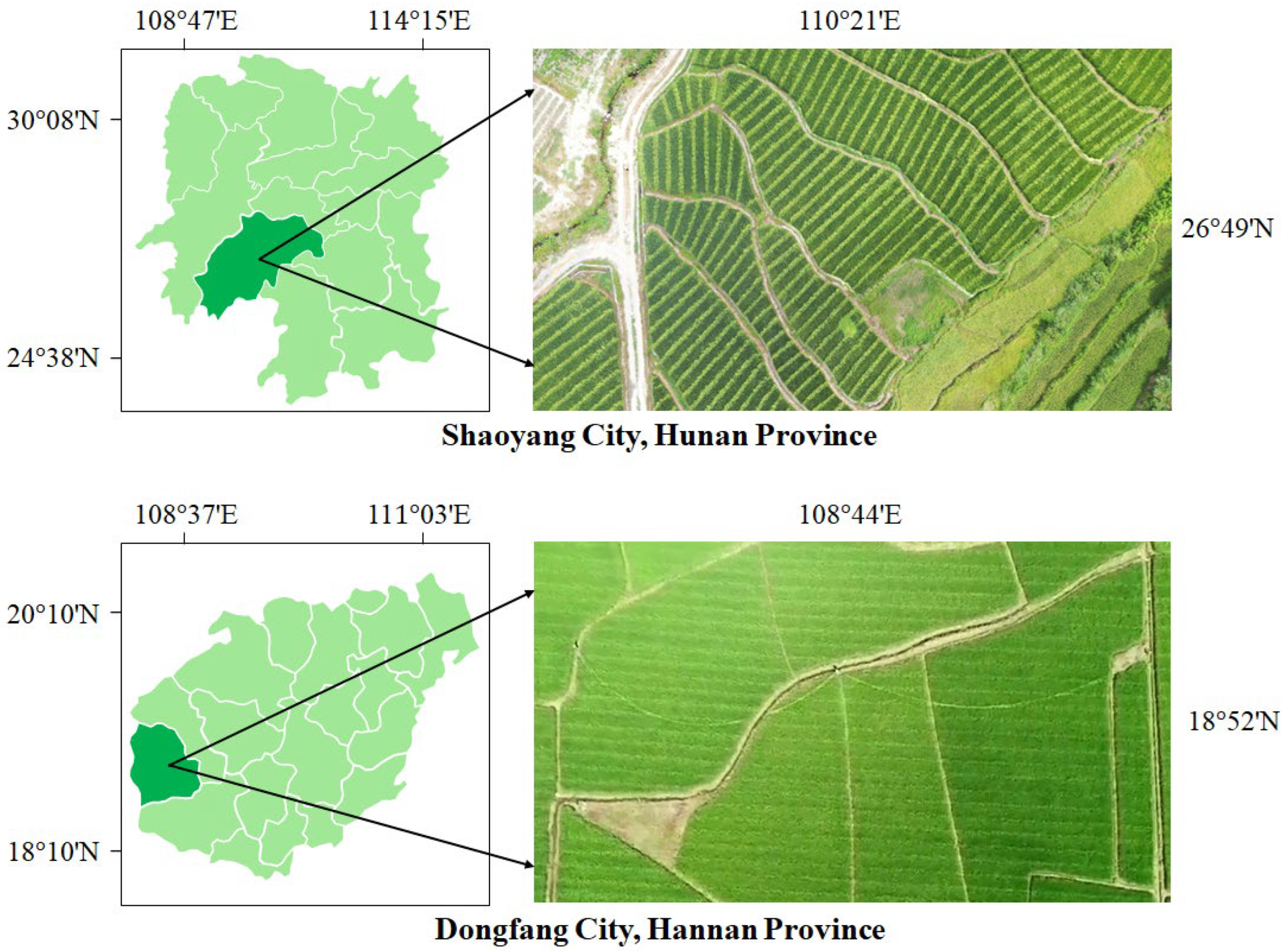
The rice flowering data were obtained in two sites (Figure 1). The first batch of sample data was collected from Hybrid Rice Breeding Base in Dongfang, Hainan Province. The second batch of data was collected from Longping Hi-tech Breeding Base in Shaoyang, Hunan Province. It was sunny and cloudless when collecting data. The temperature was between 28 °C and 31 °C. The above meteorological data were collected from a Kestrel NK5000 series handheld meteorological monitoring instrument (Nielsen-Kellerman, Boothwyn, PA, USA).

The rice in two experimental sites was cultivated by manual transplanting. Experiments were carried out during the jointing and flowering stages of rice. The male parent was planted 24 days earlier than the female parent, and the planting ratio is 2:10 between male and female plants. The male plants will be cut off early after the flowering period, which provides sufficient sunlight and nutrients to the female plants and reduces pests and disease occurrence.

2.1.2. Data Acquisition

Rice flowering information was acquired with an ASD FieldSpec^® HandHeld™ 2 spectrometer (Malvern Panalytical Ltd., Malvern, UK), which was equipped with a unique spectral acquisition instrument capable of rapid the nondestructive acquisition of spectra in the wavelength range of 325–107 nm. When measuring the hyperspectral data of the rice spikelet, it is necessary to ensure the normal operation of the handheld spectroscopic radiation spectrum so that it can accurately reflect the spectral reflection information of the rice spikelet. After the instrument startup system is loaded, the standard whiteboard with 100% reflectivity is collected for black-and-white calibration. For each data acquisition, 5 groups of hyperspectral data were collected simultaneously by a handheld spectroradiometer to reduce systematic random errors.

It is necessary to ensure that the data are collected under high light intensity and cloudless weather as far as possible to avoid the influence of external factors such as light intensity on the experimental data. In the case of cloud cover, it is necessary to wait for the cloud to disperse before continuing to collect, and at the same time, it is necessary to conduct whiteboard calibration again to ensure the accuracy of spectral data collection. In addition, when the instrument is used for collection work for a long time, even if there is no influence of external environmental factors, the whiteboard calibration needs to be carried out every 5 min to reduce the error caused by the heat generated by the instrument that occurs over long periods.

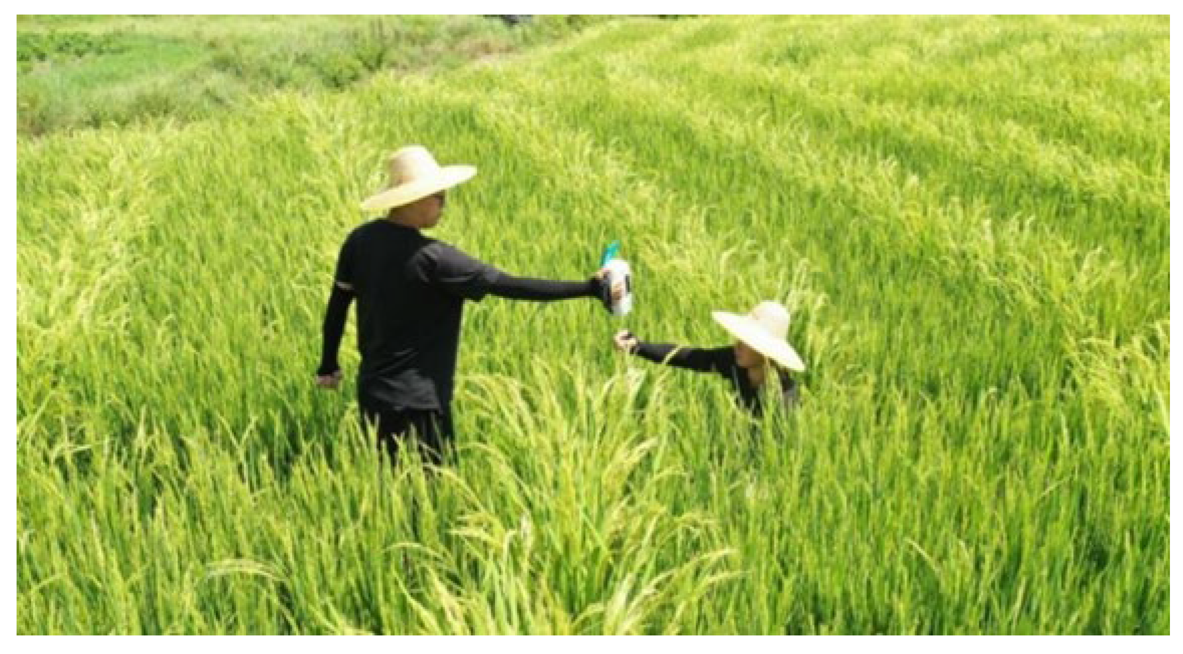
In order to ensure that the measurement is the characterization region of the rice spike, the probe of the handheld spectral radiation spectrum was put directly facing the middle of the rice spike during measurement to ensure that the rice spike is within the coverage range of the radiation spectrometer. At the same time, the instrument and the rice spike to be measured were kept a fixed distance (Figure 2).

In the Hybrid Rice Breeding Base in Dongfang, Hainan Province, 1236 hyperspectral data of rice spikelets were collected, and 1115 effective spectral data were kept for analysis after removing obvious abnormal data, with a wavelength range of 325–1075 nm. In Longping Hi-tech Breeding Base in Shaoyang, Hunan Province, 4036 hyperspectral data of spikelet were collected, and 3000 effective spectral data were obtained after removing obvious abnormal data, with a wavelength range of 325–1075 nm. The experimental data were collected in chronological order. Spectral data of the panicle region were first collected before the flowering of the male parent of hybrid rice and then during flowering time.

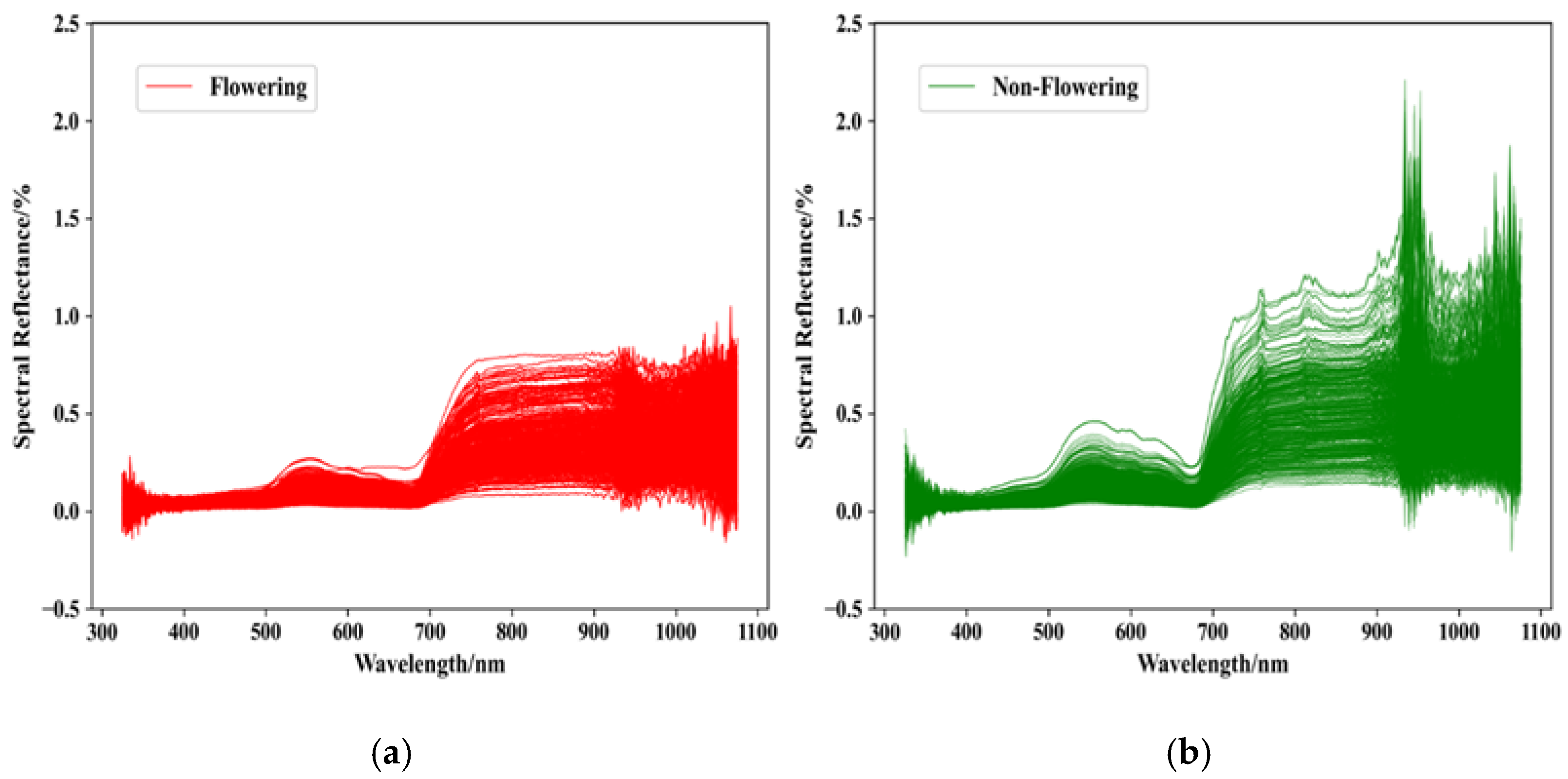
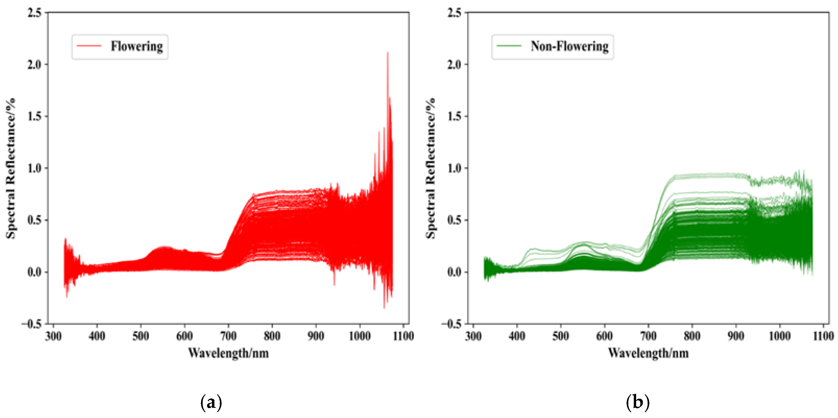
Training and test data sets were divided based on a ratio of 4:1, as shown in

Table 1. Sample size of training and test set of hyperspectral data.

	Training		Test
	Flowering	Non-Flowering	Flowering	Non-Flowering
Hainan sample	400	400	100	100
Hunan sample	400	400	100	100
All samples	800	800	200	200

. The relationship between spikelet reflectance and wavelength of rice before and after flowering is shown in Figure 3 (Hunan Province) and Figure 4 (Hainan Province). As can be seen from Figure 3a and Figure 4a, there is a large degree of overlap between spectral data of flowering and non-flowering rice, which is difficult to distinguish from artificial observation.

2.1.3. Data Preprocessing

Considering that weather fluctuation affects data accuracy, multiple pretreatments were carried out for collected hyperspectral data. Hyperspectral data of rice spikelets were preprocessed simply by using ViewSpecPro, the supporting software of the spectrometer.

• Mean calculation: During data acquisition, the ASD FieldSpec^®® HandHeld™ 2 spectrometer was set to repeatedly sample five hyperspectral curves, thus reducing the inherent error of the original spectral data; therefore, in the data preprocessing step, the collected sample data were averaged first.
• Spectral reflectance calculation: The spectral reflectance of the target can be calculated through Equation (1).

$$R_{goal}=\frac{Ra{d}_{goal}}{Ra{d}_{board}}\times R_{board}\times 100\%$$

(1)

where $R_{goal}$ on the left and right sides of the equation, respectively, represents the target spectral reflectance and the target light intensity value; the lower $Ra{d}_{board}$ represents the whiteboard light intensity value of the spectrometer and the other $R_{board}$ represents the whiteboard reflectance.

After simple preprocessing, a total of 3000 hyperspectral data of rice spikelets were obtained, including 1500 non-flowering and 1500 in full bloom. Each set of data has relative independence.

2.2. Classification Model for Detection of Rice Spikelets Flowering

Three traditional machine learning models, Random Forest (RF), Support Vector Machine (SVM), and Back Propagation (BP) neural network, as well as Convolutional Neural Network (CNN), were used to classify rice flowering using full-band spectral data. The generalization ability and deficiency of different classifiers in rice spikelet flowering detection were compared to investigate the suitable algorithm. Hyperparameters were selected using a grid search (for a given hyperparameter, set the start value, end value and interval) to test their performance on the training set and thus find the best parameter. We tested the accuracy of the model with different model hyperparameters. In RF, for the number of subtrees, the accuracy of the model between 10 and 400 was tested with 10 as the interval; for the maximum decision tree depth, the accuracy of the model from 2 to 20 was tested with 1. As in SVM, the penalty parameter C was tested for the accuracy of the SVM between [2⁻⁵, 2⁻⁴, …, 2⁹, 2¹⁰]. As in BP networks, the accuracy of the model with the number of hidden layers between [5, 10, …, 180] was tested. The CNN algorithm has a convolutional kernel size of 3 × 3 and a step size of 2.

2.2.1. RF Algorithm

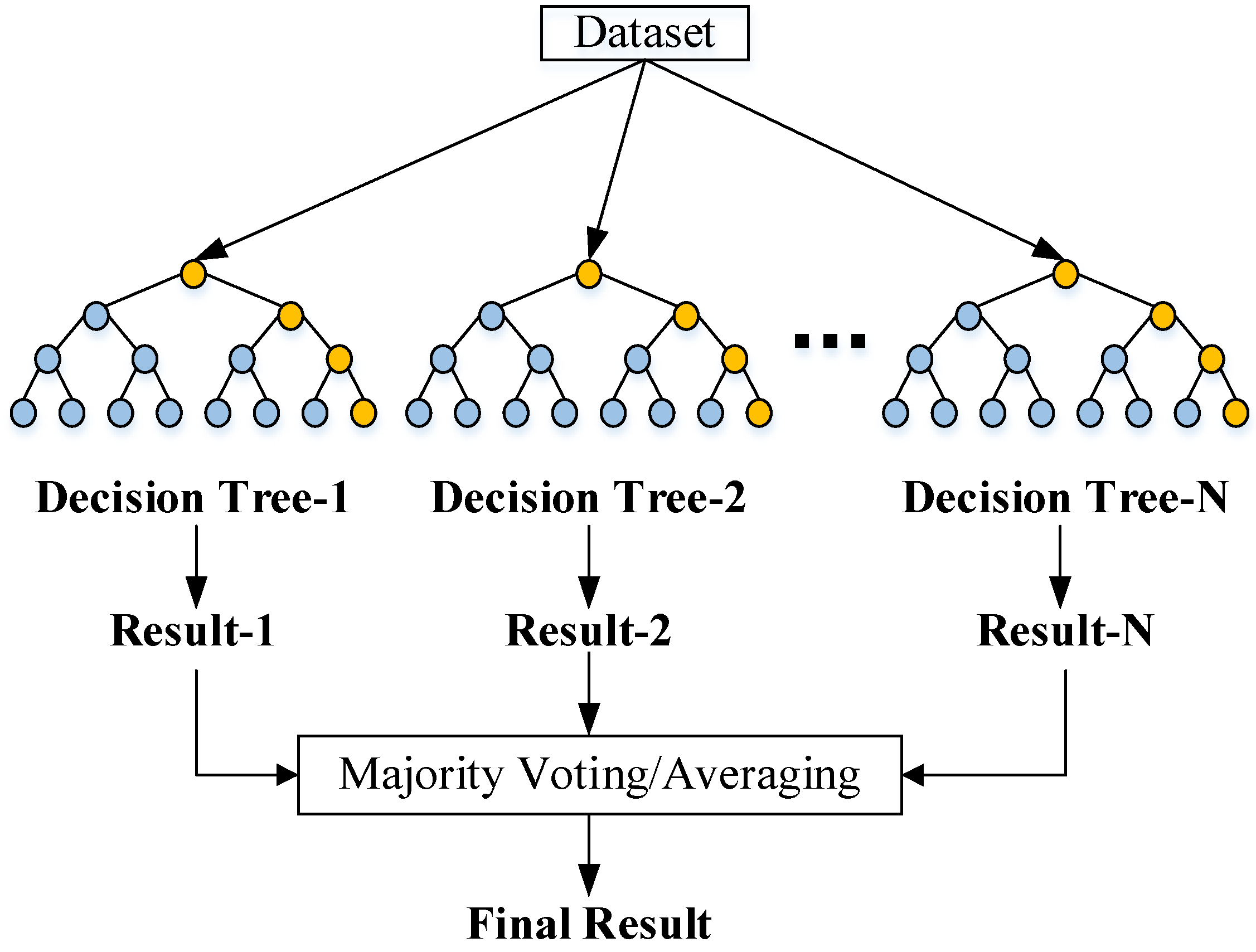
RF algorithm is widely applied to solve classification and regression type problems in many fields [14,15,16]. The algorithm adopts the ensemble learning method. By establishing a random forest (i.e., multiple classifiers), also known as a random forest decision tree, each decision tree in the random forest (i.e., each classifier) classifies the input data and then carries out the voting statistics to obtain the overall classification result.

The construction rules of the random forest [17] are as follows: (1) Defining the training sample set N: For each decision tree in the random forest, draw N training samples from the sample set in a releasing manner and arbitrarily, and define it as the training set of the decision tree; (2) assuming that N is the feature dimension of each sample, take a constant value n that is much smaller than N, select any subset of n features from N, and extract the optimal term from the n features obtained whenever the decision tree is split; (3) any decision tree in a random forest needs to grow to the maximum extent allowed by the conditions and has not undergone pruning operations during its growth and division. The algorithm flow chart is shown in Figure 5.

RF algorithm uses an integrated algorithm, which is easy to make into a parallelized method because each tree can be generated independently and simultaneously, and the random forest does not easily fall into overfitting; however, when the number of decision trees in the random forest is large, the time and space complexity of model training will be relatively high.

2.2.2. SVM Algorithm

The basic idea of the SVM algorithm is to map data to a high-dimensional feature space through nonlinear mapping and finally build an optimal classification hyperplane in the high-dimensional feature space so as to separate the nonlinear data. It can not only use a relatively simple algorithm to determine key sample feature data but also has good robustness [18].

SVM algorithm has two main principle features. SVM is targeted at linearly separable cases. When dealing with linearly indivisible cases, nonlinear features need to be transformed into linearly separable features. In this case, the low-dimensional input space linearly indivisible samples are converted into high-dimensional feature space by a nonlinear mapping algorithm and then analyzed by a linear algorithm. Based on the theory of minimum structural risk, SVM constructs the optimal classification plane in the feature space to obtain the global optimal solution for the learner. Another point is based on the principle of SVM, where a small number of support vectors determine the final classification decision result.

2.2.3. BP Neural Network

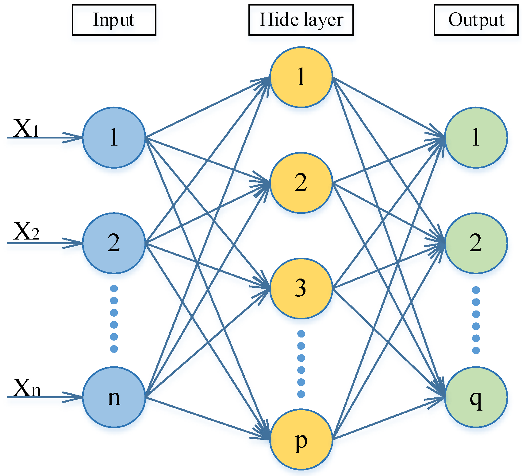
BP neural network [19] is a concept of multi-level feedforward neural network trained according to the backward error propagation algorithm. It is a widely used traditional neural network model. Its training method is an error back propagation algorithm, through which the weight and threshold of the neural network are constantly adjusted and modified to obtain the minimum mean square error value, and finally results in the optimal fitting degree of the data. Its network model topology is composed of three parts: input layer, hide layer and output layer. Figure 6 gives a brief demonstration on the flow chart of BP neural network, where X₁, X₂, X_n represent the input hyperspectral reflectance consisting of 751 channels. BP neural network algorithm consists of two parts: signal forward conduction and error result reverse conduction.

The function of the input layer of the BP neural network is to transmit the input information received from the outside to the middle layer, and each neuron in the middle layer transforms the input information. According to the demand for information transformation processing ability to design a single hidden layer structure or more hidden layer structure, then through the last hidden layer, the processed information is transmitted to the output layer for subsequent processing. Finally, the output layer of the neural network will output the information processing results obtained in the neural network algorithm. At this point, if there is a difference between the actual output value and the expected output value, the error will enter the reverse conduction stage. The weight will be modified and adjusted in all layers of the neural network according to the gradient descent method, and the error will be reverse transmitted through the output layer to the middle layer and then to the input layer. The training process of a neural network that is constantly repeating information forward conduction and error reverse conduction of weights within every level continuously in the process of adjustment. The training process continues until the error of the neural network output achieves an acceptable level or is set in advance of the neural network to build learning.

2.2.4. CNN Algorithm

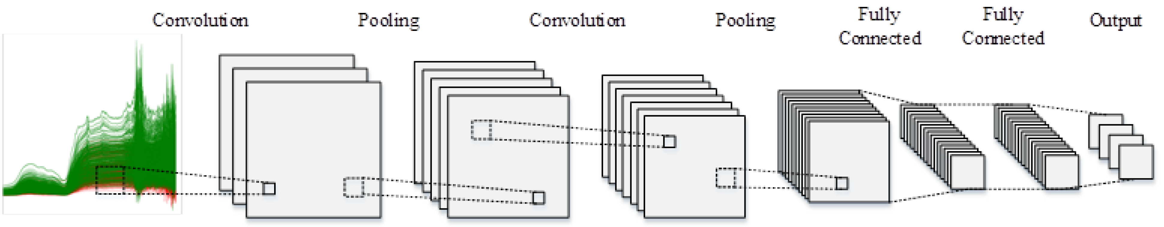
CNN is one of the representative algorithms of deep learning. It is a type of feedforward neural network with a deep structure, including convolution computation. The CNN algorithm has been widely used in various fields of classification, retrieval, identification (classification and regression), segmentation, feature extraction, key point positioning (posture recognition) and other scenes [20]. The structure of CNN is usually composed of an input layer, convolutional layer, pooling layer, fully connected layer and output layer. Figure 7 shows the classical structure of the CNN algorithm.

The input layer of the CNN inputs the target detection sample into the CNN structure. When the sample data are fed into the input layer, the computer treats the input as a matrix and performs a series of transformations on the matrix before feeding it into the next layer of the structure. The convolutional layer is a unique structure of the CNN algorithm model and a core layer of the whole neural network, which produces most of the computational work. The structure used by the combination of the convolutional layer and the pooling layer can be set repeatedly in the hidden layer. The function of the convolution layer is to deepen the original matrix, and the nodes processed by the convolution layer will obtain a deeper matrix. The pooling layer extracts the main information of the samples based on the principle of local connectivity of the features in order to reduce the amount of data processing. It does not change the depth of the 3D matrix, but the size of the matrix is reduced, thus reducing the parameters in the whole neural network and the number of training dimensions. The fully connected layer is a structure that weighs all the neurons between the two layers, and the last output layer serves as the target result. These two parts are generally configured at the end of the CNN model. CNN uses original samples as input, which can effectively learn corresponding features from a large number of samples and avoid a complex feature extraction process. CNN algorithm can also be used for the classification of 1D data by varying the size of the convolutional kernel.

2.3. Data Dimensionality Reduction Algorithm

Although hyperspectral data receive high classification accuracy under the above four classification models, the original data have a high dimension and a slow operation rate; therefore, dimensionality reduction was performed to improve the running speed and accuracy of the model. Two commonly used dimensionality reduction methods were selected in this study. Rice flowering detection was then conducted on the basis of feature dimensionality reduction in order to obtain better results.

2.3.1. Principal Component Analysis

Principal Component Analysis (PCA) [21] is the most widely used data dimensionality reduction algorithm. The main idea of the PCA algorithm is to map n-dimensional features to k-dimensional features. These new orthogonal features, also called principal components, are reconstructed from the original n-dimensional features. The job of PCA is to find a set of mutually orthogonal axes in turn from the original space, and the choice of new axes is closely related to the data itself. The first new axis is selected in the direction of the greatest difference in the original data. The second axis is selected in a plane orthogonal to the first axis to maximize the variance. The third axis is selected in a plane orthogonal to the first and second axes to maximize the variance. By analogy, n such axes are obtained. The new axis obtained in this way contains most of the variance of the first k axes, and the variance of the last axis is almost zero. This is equivalent to reducing the dimensionality of the data features by retaining only the dimensional features that contain most of the variance and ignoring the dimensional features that contain almost zero variance.

By calculating the covariance matrix of the data matrix and then obtaining the eigenvalue and eigenvectors of the covariance matrix, the matrix consisting of the eigenvectors corresponding to the k features with the largest eigenvalue (i.e., the largest variance) is then selected. The data matrix is transformed into a new space to achieve dimensionality reduction in data features. At present, there are mainly two methods to obtain the eigenvalue and eigenvector of covariance matrix: the PCA algorithm based on eigenvalue decomposition covariance matrix and the PCA algorithm based on the SVD decomposition covariance matrix.

2.3.2. Genetic Algorithm

A Genetic Algorithm (GA) is a computational model that simulates the biological evolution process of natural selection and genetic mechanism in Darwin’s biological evolution theory. It is a method to find out the optimal solution by simulating the natural evolution process. When solving complex combinatorial optimization problems, it usually obtains better optimization results faster than some traditional optimization algorithms. GA has been widely used in combinatorial optimization [22], machine learning [23], signal processing [24], adaptive control [25] and artificial life.

GA starts with a population that represents a set of possible solutions to a problem. A population consists of a certain number of genetically coded individuals. Each individual is actually a chromosomal entity with characteristics. After the initial population is generated, according to the principle of survival of the fittest, it evolves generation by generation to produce better and better approximate solutions. In each generation, individuals are selected according to their fitness in the problem domain, and combined crossover and mutation are performed with the help of natural genetic operators to generate a population representing a new set of solutions. This process will produce a metapopulation similar to natural evolution, which is more adaptable than its predecessors, and the best individuals in the previous generation are decoded and can be used as approximate optimal solutions to the problem.

2.4. Evaluation of Algorithm Accuracy

The prediction results of the model for rice flowering detection were as follows: TP (true positive): positive samples were correctly predicted as positive samples, i.e., the data of spikelet flowering were predicted as flowering. FP (false positive): a negative sample is incorrectly predicted as a positive sample, i.e., a non-flowering spikelet is predicted as flowering. TN (true negative): negative samples were correctly predicted as negative samples, i.e., non-flowering data were predicted as non-flowering. FN (false negative): positive samples were wrongly predicted as negative samples, i.e., the data on flowering of spikelets were predicted as non-flowering.

The evaluation indexes are precision (the proportion of the total number of rice spikelets flowering that can be correctly detected) and recall (the proportion of correctly predicted rice spikelets flowering in total actual flowering), which can be calculated by Equations (2) and (3), respectively.

$$Precision=\frac{TP}{TP+FP}$$

(2)

$$Recall=\frac{TP}{TP+FN}$$

(3)

3. Results

3.1. Classification Accuracy before Feature Dimensionality Reduction

The 800 sets of 751-dimensional hyperspectral data from Hainan, 800 sets of 751-dimensional data from Hunan and 1600 sets of 751-dimensional mixed data from Hainan and Hunan were input to the traditional classifiers and deep learning model for training. A total of 200 sets of Hainan data, 200 sets of Hunan data, and 400 sets of mixed data were used for validation. The correlation results of each group are shown in Figure 8.

As can be seen from Figure 8, the precision and recall rate of validation from the Hainan data set ranges from 36% to 100%. BP neural network model received the highest score, and the accuracy of both evaluations obtained by training with the Hainan data set reached 100%. The RF algorithm obtained the lowest score. Its accuracy of training using the Hunan data was 36–45%. The RF scores for the Hunan validation ranged from 47% to 93%. Among the four models, the highest score was achieved by the CNN algorithm model, which reached 87–90% when trained with mixed data. The lowest scores were also observed in the CNN model, which resulted in 47–62% when trained with Hainan data. The score range of the mixed validation data was 55–95%. The highest score was obtained by the CNN model. When the mixed data were used for training, the evaluation accuracy of the CNN model reached 93%. The lowest was the RF model, which was trained with Hunan data with an accuracy of 60–61%.

The reason that the RF model performed the worst may lie in the fact that it does not provide a continuous output. When performing regression, it cannot make predictions beyond the range of the training data set. This leads to overfitting when modeling data with some specific noise, or there are many similar decision trees that mask the true results. The CNN model performed the best. The reason may be explained by the fact that convolutional neural networks have a parameter sharing mechanism. This mechanism greatly reduces the number of parameters of the network and trains a better model with fewer parameters, which can effectively avoid overfitting. The sparsity of the network connections allows the data to be given better and more effective weights.

3.2. Classification Accuracy after Feature Dimensionality Reduction

3.2.1. Feature Extraction with PCA algorithm

For each group of 751-dimensional data, the PCA algorithm was used to extract features from the data and the 751-dimensional data were then downscaled to 200 dimensions by optimizing the parameters. After dimensionality reduction, the 800 groups of 200-dimension Hainan data, 800 groups of 200-dimension Hunan data and 1600 groups of 200-dimension mixed data from Hainan and Hunan were input to traditional classifiers and deep learning model for training. Another 200 groups of Hainan data, 200 groups of Hunan data were used and 400 groups of mixed data from Hainan and Hunan were used for validation. The final accuracy result is shown in Figure 9.

As can be seen from Figure 9, the correlation range of Hainan validation data was 21–100%, of which the BP model has the highest accuracy. When training with Hainan data, the precision and recall rate are both 100%. The lowest score was observed in the RF model, which was trained with Hunan data, and its accuracy was only 21–22%. The score range for Hunan validation data was 46–100%, in which the BP model received the highest accuracy of 96–100% when trained with the mixed data set. The lowest accuracy was observed in the SVM model, which was only 50–60% when trained with Hainan data. The scores for the mixed validation data ranged from 29–99%, with the highest detection model being the BP model, trained using mixed data, at 96–99%, and the lowest being the CNN model, trained using Hunan data, at 29–33%.

Compared with the original data before dimensionality reduction, the accuracy of the trained models was improved. The best BP algorithm model can handle the data of Hainan up to 100%, which is relatively stable and has good generalization ability. The results of the Hunan validation data have a relatively large improvement, with the highest score of 96–100%. In the four algorithm models with PCA feature extraction, some performance improves and some performance worsens.

3.2.2. Feature Selection with GA

The 751-dimensional original data of Hainan, Hunan and mixed data were used for GA feature selection. After dimensionality reduction, the three sets of data were downscaled to 350, 384 and 362 dimensions by parameter optimization, respectively. Then, 800 sets of 350-dimensional Hainan data were input to the traditional classifier and deep learning model for training. The 200 sets of 350-dimensional Hainan data, 200 sets of 350-dimensional Hunan data and 400 sets of 350-dimensional Hainan–Hunan mixed data were used for validation. The 800 sets of 384-dimensional Hunan data and 1600 sets of 362-dimensional mixed data also performed the same operation. Final accuracy results are shown in Figure 10.

By observing the results in Figure 10, the precision and recall rate of Hainan validation data ranged from 40–100%. Among Hunan data, the highest score goes to RF and BP models with 97%–100%. The lowest scores lie in the RF model, which was only 40–54% based on the training results of Hunan data. The scores of the Hunan validation data ranged from 48% to 95%. The optimal model is the CNN model, which was trained with the Hainan–Hunan mixed data, reaching 86% to 89%. The lowest is the SVM model, which received 50–71% based on the training results using Hainan data. The scores of mixed validation data ranged from 54% to 94%, and the highest was the CNN model, which was trained with mixed data from Hainan and Hunan, reaching 92% to 93%. The lowest was the SVM model, which was trained with Hunan data and its accuracy was only 54–68%.

Compared with the original data before dimensionality reduction, the dimensionality reduction data after GA feature selection received about 2% lower accuracy, but the input dimension was reduced by nearly half, which reduced a lot of operations. The less effective model was the SVM model, and the best one was the BP model.

3.2.3. Combination of PCA Feature Extraction and GA Feature Selection

Feature extraction was performed first on the 751-dimensional data from Hainan using the PCA method. Then, the original 751-dimensional data generated new 751-dimensional feature data in order of importance. Finally, GA was performed to reduce the new 751-dimensional data through feature selection to 404-dimensional data. Hunan data and mixed data were similarly reduced to 369 and 388 dimensions by performing the above operations, respectively.

After dimensionality reduction, 800 sets of 404-dimensional Hainan data were input to the traditional classifiers and deep learning model for training. At the same time, 200 sets of 404-dimensional Hainan data, 200 sets of 404-dimensional Hunan data, and 200 sets of 404-dimensional Hainan-Hunan mixed data were used for validation. The same training and validation operations were performed for the 800 sets of 369-dimensional Hunan data and the 1600 sets of 388-dimensional mixed data. The final results are shown in Figure 11.

The results in Figure 11 show that the precision and recall rate of Hainan validation data ranged from 18–100%, among which the optimal model was the RF model trained by Hainan data and the BP model trained by mixed data. The evaluation results of these two models were 99%. The RF model trained by Hunan data performed the worst with an accuracy of 18–19%. The scores of the Hunan validation data ranged from 49% to 98%. The BP model trained by mixed data reached 92% to 98%, while the CNN model trained by Hainan data only reached 50% to 89%. The score of mixed validation data was 32–96%. The BP model trained by mixed data received an accuracy up to 95–96%. The lowest scores lie in the CNN model trained with Hunan data—the accuracy was only 32–35%.

After PCA feature extraction for the original data and then GA feature selection, the result does not combine the advantages of the two dimensionality reduction methods well. The result is even lower than that of the original data; therefore, the combination of PCA and GA methods for dimensionality reduction is not applicable for hyperspectral data identification of flowering and non-flowering rice spikelets.

4. Discussion

This study innovatively proposed the application of hyperspectral technology to detect the flowering state of rice spikelets and made full use of the advantages of hyperspectral technology to obtain better detection results. Compared with artificially judging the flowering state of rice spikelets, the detection method combining hyperspectral technology and machine learning is faster and more accurate. In the future, the results obtained in this study can be made into hyperspectral sensors, which can realize remote flowering detection, which greatly saves labor costs.

Zhang et al. [26] obtained rice spikelet images from a visible light camera. Series Otsu (SOtsu) was applied in tandem to extract the spikelet anthers through the visible light blue channel. In the meantime, deep learning models, such as FasterRCNN and YOLO-v3, were used to identify the spikelet anthers and the opening spikelet hull. The most suitable method was selected for flowering characteristics detection to compare the precision, recall and the F1 coefficient of different models. Results showed that the precision, recall rate, F1 coefficient and Pearson correlation coefficient of the FasterRCNN model in spikelet hull detection were 1, 0.97, 0.98 and 0.993, respectively, while those of SOtsu in spikelet anthers detection were 0.92, 0.93, 0.93 and 0.936, respectively. It inferred that the SOtsu and FasterRCNN models were both capable of rice flowering detection, but the opening spikelet hull was more suitable than the spikelet anthers for the rice flowering features detection with the deep learning model; however, compared with the detection method with a visible light camera, the hyperspectral data collected in this study carries more effective information and is easier to process. The hyperspectral data can clearly perceive the changes in spectral reflectance caused by the subtle changes in the flowering process of rice glumes. In addition, the application of machine learning algorithms to build classification models can make full use of the spectral information carried by the hyperspectrum, making the predictive ability of the models more powerful compared to the application of other detection methods.

Due to the overlapping signature and negligible difference between flowering and non-flowering spectra for both Hainan and Hunan locations, we used full-band reflectance data for modeling. In addition, the result of data dimensionality reduction through the GA algorithm shows that it contributes to the detection of rice flowering status in almost the whole waveband range, and the contribution values do not differ significantly.

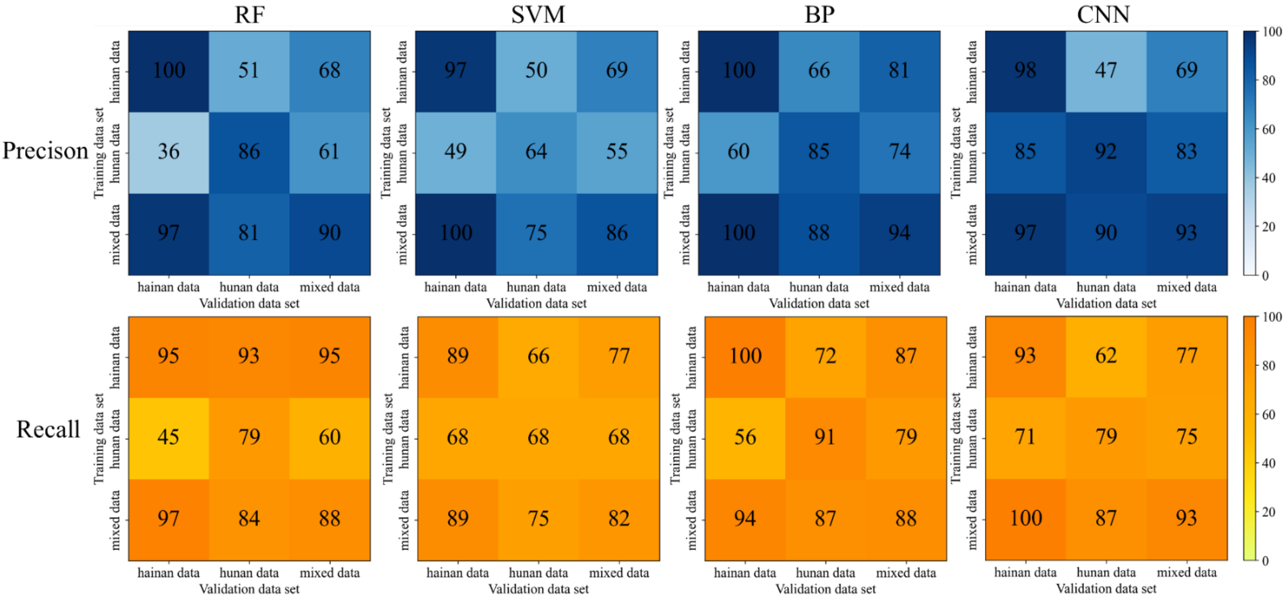
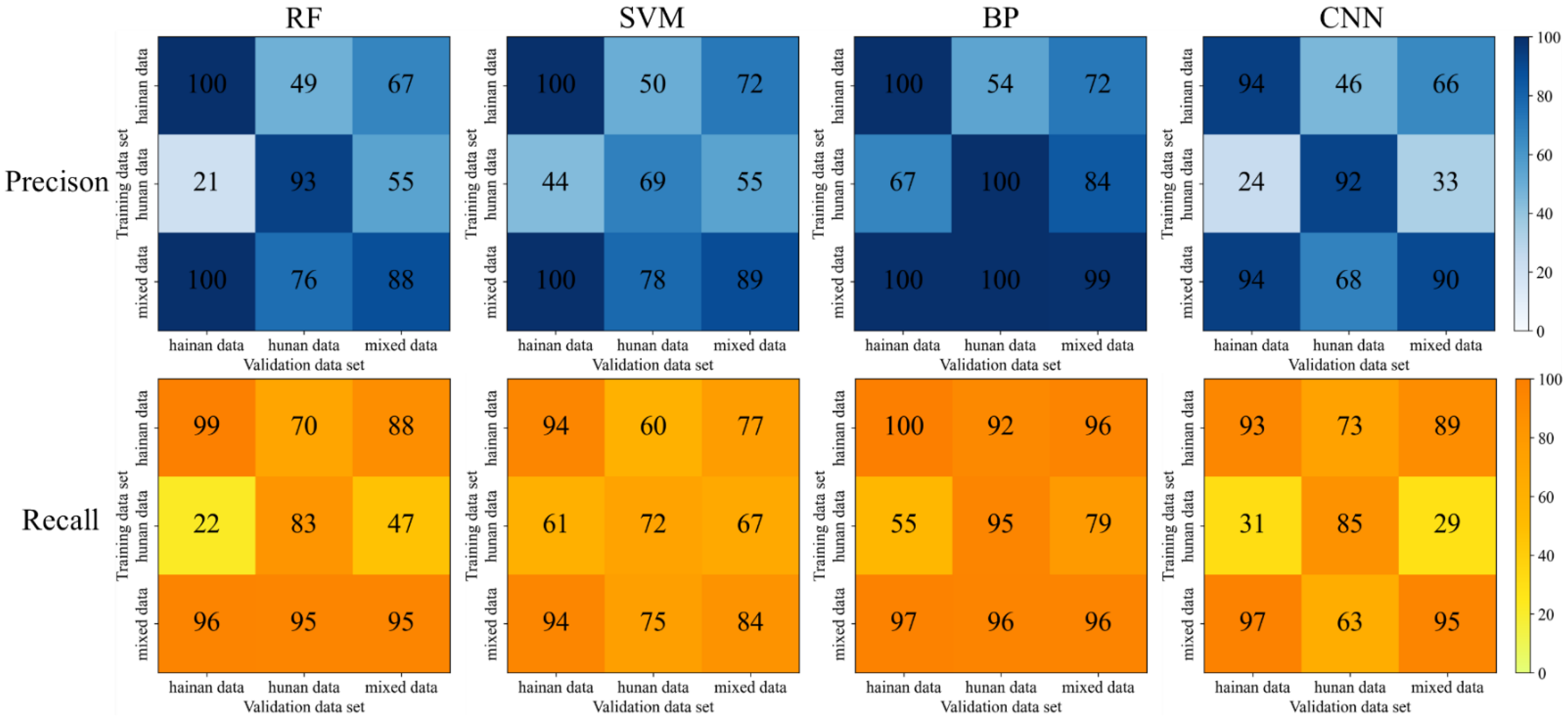
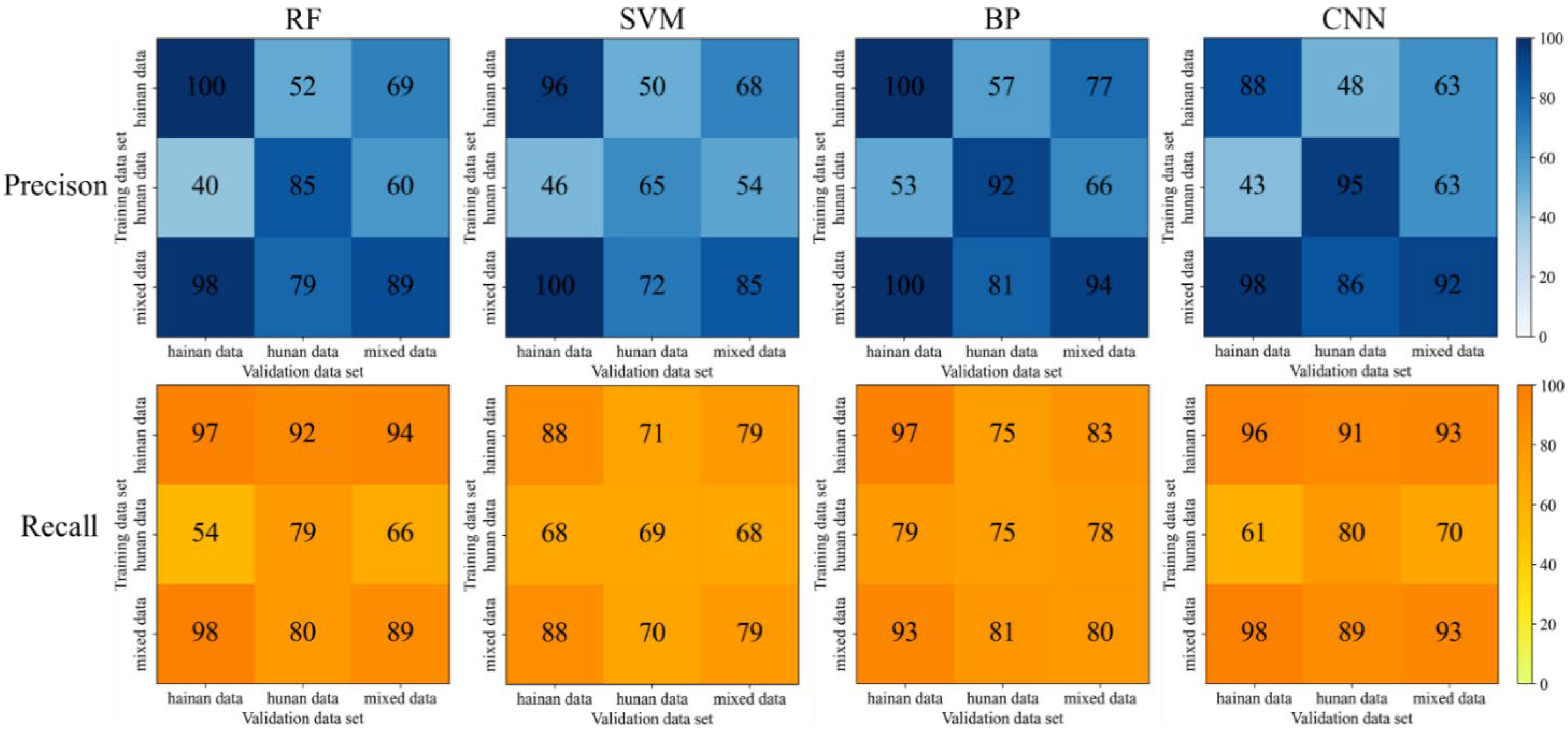
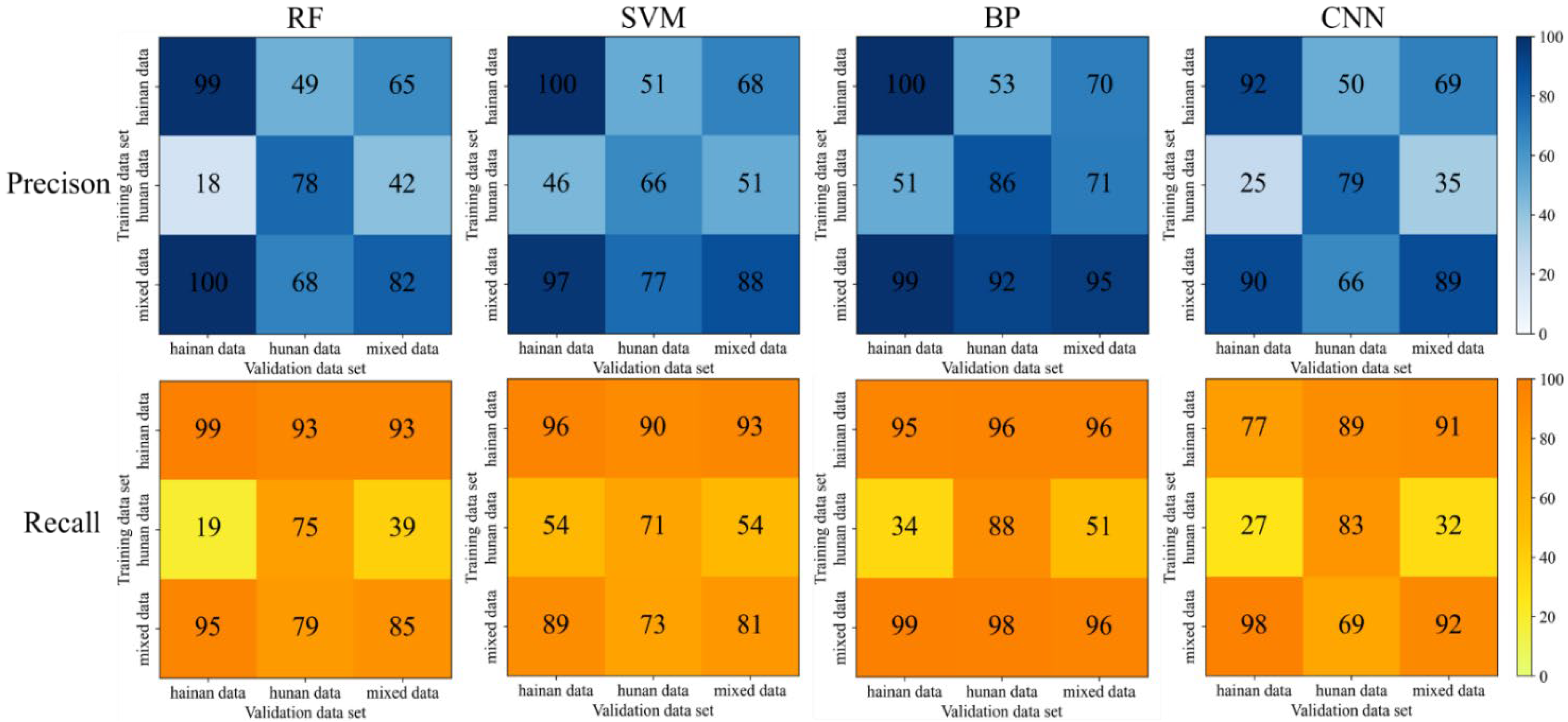
Among the four data processing methods, PCA feature extraction has the best result in terms of overall effectiveness, followed by the original data modeling, the PCA and GA combination and the GA feature selection. Among the PCA feature extraction processing methods, the BP model achieved the highest evaluation accuracy. The precision and recall rate is between 96% and 100% when trained by Hainan and mixed data, indicating that the BP model has an excellent classification effect and strong generalization ability for rice flowering detection. Although the results derived from the GA feature selection did not improve, the dimensionality of its input was reduced by nearly half while it still maintained the acceptable score, indicating that nearly half of the 751-dimensional data were not very useful for the classification of this study and could be eliminated. From the selected bands, their effective bands were basically evenly distributed, with some concentration in individual places. Most likely, it results from the similarity of the adjacent bands. After GA feature selection, the redundant information was removed to ensure the efficiency of the information; therefore, the feature reduction serves to remove the redundant and interfering features in feature bands, which in turn improves the accuracy of the processing results.

Among the four classification models, the BP algorithm model achieves a comprehensively better result, followed by the CNN model, RF model and SVM model. The results obtained by the BP algorithm model may be due to the (1) nonlinear mapping ability: BP neural network essentially realizes a mapping function from input to output; mathematical theory proves that the three-layer neural network can approach any nonlinear continuous function with arbitrary accuracy, which has strong nonlinear mapping ability. (2) Self-learning and self-adaptive ability: during training, BP neural network automatically extracts “reasonable rules” between input and output data through learning and adaptively memorizes the learning content into the weight of the network with high self-learning and self-adaptation ability. (3) Generalization ability: in the design of the pattern classifier, it cares about whether the network can correctly classify the patterns not seen before or those with noise pollution after training and has the ability to apply the learning results to new knowledge. (4) Fault tolerance: BP neural network will not have a great impact on the global training results after its local or partial neurons are damaged; the system can still work normally when local damage occurs and it has a certain fault tolerance. The reason for the relatively poor results of the CNN algorithm may be that it learns by convolution, which may lose some parts of the data and ignore the correlation between the local and the whole, thus affecting the results. RF model may be overfitted for noisy data. SVM model may not be optimal for the selection of parameters, which can only be chosen empirically and through human selection, with a certain degree of arbitrariness.

From the results of multiple processing, Hainan data have a good classification effect, probably because there is a more obvious difference between the flowering and non-flowering bands in Hainan data; however, the classification effect of Hunan data is poorer, probably because there is more noise in Hunan data or the difference between the flowering and non-flowering bands is not obvious, which makes it more difficult to classify. Comparing the generalization ability of Hainan data alone with that of Hunan data, the classification algorithm has a better generalization ability. The BP algorithm model in PCA feature extraction processing has improved generalization ability for mixed data, and the results of Hunan validation data can have a 1% improvement compared with the training results of Hunan data alone. There is a big difference between Hainan data and Hunan data. When applying the model trained by one site to validate the data from another site, the precision and recall rate is basically around 50%.

In summary, the algorithm adopted in this study is quite effective in detecting the hyperspectral data before and after rice flowering. Considering the operational problems in the data acquisition process and the influence of the objective physical environment on the instrument may cause interference to the acquisition of rice flowering hyperspectral data, there will be some influence on the results of machine identification. In addition, the sample data set adopted in this study is still small, and the algorithm should be further explored to improve the generalization ability of the algorithm for the identification of different varieties of rice flowering in different regions.

5. Conclusions

This study proposed to acquire rice spikelet flowering information using hyperspectral technique and machine learning in order to meet the needs of hybrid rice pollination rapidly and automatically. The hyperspectral data of rice before and after flowering were collected by a spectroradiometer. Based on traditional machine learning algorithms and deep learning algorithms, preliminary classification models were constructed to identify rice flowering status. The traditional classifiers used in this study include the SVM algorithm, RF algorithm and BP network. The deep learning classifier is the CNN algorithm. By comparing the four algorithm models, it can be found that the CNN algorithm model has the best accuracy in the detection of rice flowering. The average accuracy and recall rate of the model is 93% when using the data collected from two locations mixed as data input. Three methods, PCA feature extraction, GA feature selection and the combination of PCA and GA algorithm, were applied to transform hyperspectral data into a new feature space based on the feature dimension reduction method and then carried out the classification of rice flowering in this space combining with machine learning algorithms. It can be found that the PCA algorithm was applied to feature extraction of rice spikelet spectral data, which could make full use of the effective information in the spectral band and improve the accuracy and recall rate of the model. Although the GA algorithm did not improve the accuracy and recall rate of the model, it reduced the dimension of model input information and reduced the complexity of model calculation while maintaining the accuracy of the model. The feature extraction method combined with PCA and GA failed to integrate the advantages of the two algorithms, and its accuracy even decreased when compared with the preliminary classification model based on machine learning algorithms. By comprehensively comparing the combination of different feature dimensionality reduction methods and classification models, the optimal model was constructed by using the data processed by the PCA feature extraction method and then classified by the BP algorithm. The accuracy and recall rate of mixed data is 96–100%. The experimental results show that the hyperspectral technology and machine learning algorithm proposed in this study can effectively obtain the flowering status of rice spikelets, which is expected to provide decision-making information for timely pollination in mechanized seed production of hybrid rice.