Weedy Rice Classification Using Image Processing and a Machine Learning Approach

Abstract

Weedy rice infestation has become a major problem in all rice-growing countries, especially in Malaysia. Challenges remain in finding a rapid technique to identify the weedy rice seeds that tend to pose similar taxonomic and physiological features as the cultivated rice seeds. This study presents image processing and machine learning techniques to classify weedy rice seed variants and cultivated rice seeds. A machine vision unit was set up for image acquisition using an area scan camera for the Red, Green and Blue (RGB) and monochrome images of five cultivated rice varieties and a weedy rice seed variant. Sixty-seven features from the RGB and monochrome images of the seed kernels were extracted from three primary parameters, namely morphology, colour and texture, and were used as the input for machine learning. Seven machine learning classifiers were used, and the classification performance was evaluated. Analyses of the best model were based on the overall performance measures, such as the sensitivity, specificity, accuracy and the average correct classification of the classifiers that best described the unbalanced dataset. Results showed that the best optimum model was developed by the RGB image using the logistic regression (LR) model that achieved 85.3% sensitivity, 99.5% specificity, 97.9% accuracy and 92.4% average correct classification utilising all the 67 features. In conclusion, this study has proved that the features extracted from the RGB images have higher sensitivity and accuracy in identifying the weedy rice seeds than the monochrome images by using image processing and a machine learning technique with the selected colour, morphological and textural features.

1. Introduction

Weedy rice refers to a weed species in a rice field. Weedy rice infestation is not just a local problem, as it has been reported worldwide and has spread to many rice-growing-field countries such as the USA, Europe, China and South East Asian countries [1,2,3,4]. In Malaysia, weedy rice has become a significant constraint to rice production. Shifting rice culture from hand transplanting to direct-seeded rice has introduced weedy rice problems [5,6,7] in Malaysia. Weedy rice is a weed with taxonomic and physiological similarities to the cultivated rice seed. In major rice granaries in Malaysia, weedy rice plants have become competitive with cultivated rice and can be dominant throughout the rice planting field [8]. The impact of a weedy rice infestation reduces the yield potential of a rice field to 60% [9]. The weedy rice has an earlier maturity stage than the cultivated rice, and once the grain matures, it is easily shattered and remains dormant in the soil. Selective herbicides have been introduced, such as imidazolinone under the Clearfield^® rice programme, to control the weedy rice infestation. However, the potential of soil leaching and the emergence of the resistant weedy rice has been found to nullify the efficacy of the herbicide [8].

The leading authority in releasing certified rice seeds to farmers inspects the seed quality manually by counting and visually inspecting each seed sample produced by the seed producer. The manual method is challenging as it depends on the experience of the laboratory personnel to identify the weedy rice seed. Due to the taxonomic and physiological similarities between the weedy rice and the cultivated rice seeds, the physical separation of the weedy rice seeds during processing to meet the standard specifications of the certified seeds has its limitations. Reducing and avoiding weedy rice contamination in seed production is crucial for future planting seasons. Therefore, a more accurate identification system is needed to identify the unwanted weedy rice seeds from the cultivated rice seeds to fulfil the urgency of providing high-quality certified rice seeds.

Recently, the computer vision technique has grown to meet the demand for fast and accurate grain quality evaluation, as reviewed by [10]. The application of computer vision in seed grading and quality inspection [10,11,12,13,14,15,16,17] has been proven by many researchers. The use of computer vision combined with pattern recognition and automatic classification tools enables the analysis of massive data volumes for quick and accurate decision making [10]. The classification algorithm provided by the machine learning techniques involves training the input features to identify the intended class of the grain.

Within the domain of rice seed grain studies, Chaugule and Mali [18] employed a neural network and used specific rice shape, colour and texture features to classify four Indian rice seed varieties based on the RGB images captured by a machine vision setup. In a further experiment, Chaugule and Mali [19] identified new features related to the front–rear and horizontal–vertical rice seed angle to discriminate the same varieties, which increased the classification accuracy to 97.6%. Meanwhile, Singh and Choudary [20] classified four rice grain varieties using various machine learning techniques and using colour, texture and wavelet decomposition features, and obtained an average accuracy of 96%. Kuo et al. [21] used specific rice seed grain features such as the grain body, sterile lemmas and brush extracted from a Fourier descriptor alongside the standard morphology, colour and texture features to classify 30 rice grain varieties from the five genetic subpopulations. The grain-variety identification was based on the sparse-representation classification that achieved an average accuracy of 89.1%. Huang and Chien [22] found that three Taiwanese rice seed varieties that have a very similar appearance could be classified up to 97.35% using a back-propagation neural network. They utilised special geometric features calculated on the chaff tip, glume, lemma and palea of the seed. Besides deriving special rice seed features, Cinar and Koklu [23] utilised only morphological features, trained seven machine learning classifiers, and had the highest accuracy of 93.02% from the logistic regression model. Meanwhile, Anami et al. [24] used a trained support vector machine, KNN and back-propagation neural network to classify the adulteration of a bulk rice seed sample using only texture and colour features with an average accuracy of 97.26%. All the above research used RGB images as the input to a machine learning system for rice seed classification. Other than RGB images, [25,26] used greyscale images obtained from a flatbed scanner to simplify the image processing methodology and provide a low-cost application.

Studies of weedy rice have mainly focused on genetic introgression and evolution [27,28,29,30] management strategies including control [1,3,6,7,8,13] and plant morphology [31]. Very few studies involve identifying the weedy rice seed by using machine vision and machine learning techniques. The current manual identification technique, relying on the physical separation based on seed length and physical appearances seen by human eyes, does not guarantee an effective weedy rice separation. A study by Aznan et al. [32] indicated there is potential for weedy rice seed variants to be classified from the cultivated rice seed variety (the MR263 cultivated rice seed variety) using machine vision and Discriminant Analysis with an accuracy of 96%; however, this study only used the morphological features of the seed and tested only one variety. Further, the physical appearance and other potential parameters were available, such as the colour of the seed and textural features, which can be captured in an image and extracted using image processing. These features provide the advantage of understanding the external quality parameters of agricultural samples. The combination of morphology, colour and texture parameters extracted from seed images can be expected to increase the classification rate of weedy rice using various machine learning techniques.

Therefore, this study aimed to explore the possibility of classifying the weedy rice seed from the cultivated rice seed varieties using a machine vision and machine learning technique. Specifically, the morphology, colour and texture features of the rice seed were extracted and used to differentiate weedy rice seed variants and Malaysian cultivated rice seed varieties.

2. Materials and Methods

2.1. Sample Collection

In this study, five varieties of the cultivated rice (CR) seed and weedy rice (WR) seed variants were obtained from the Department of Agriculture, Teluk Cengai, Kedah, where the Paddy Seed Certification Scheme services are conducted in the Northern area of Malaysia. The CR seed varieties, namely MR297, MR220 CL2, MR219, UKMRC2 and UKMRC8, were locally produced to fulfil the planting demands for the certified rice seeds. A total of 7350 CR seeds were used, with 1470 seed kernels for each variety. About 895 WR seeds managed to be sampled by the laboratory personnel, which were obtained during the search for WR from the CR seed samples. The samples were then divided into 70% for training (5772 seeds, where 1029 seeds were used for each CR variety and 627 WR seeds) and 30% (2473 seeds, where 441 seeds were used for each CR variety and 268 WR seeds) for testing datasets.

2.2. Machine Vision Setup

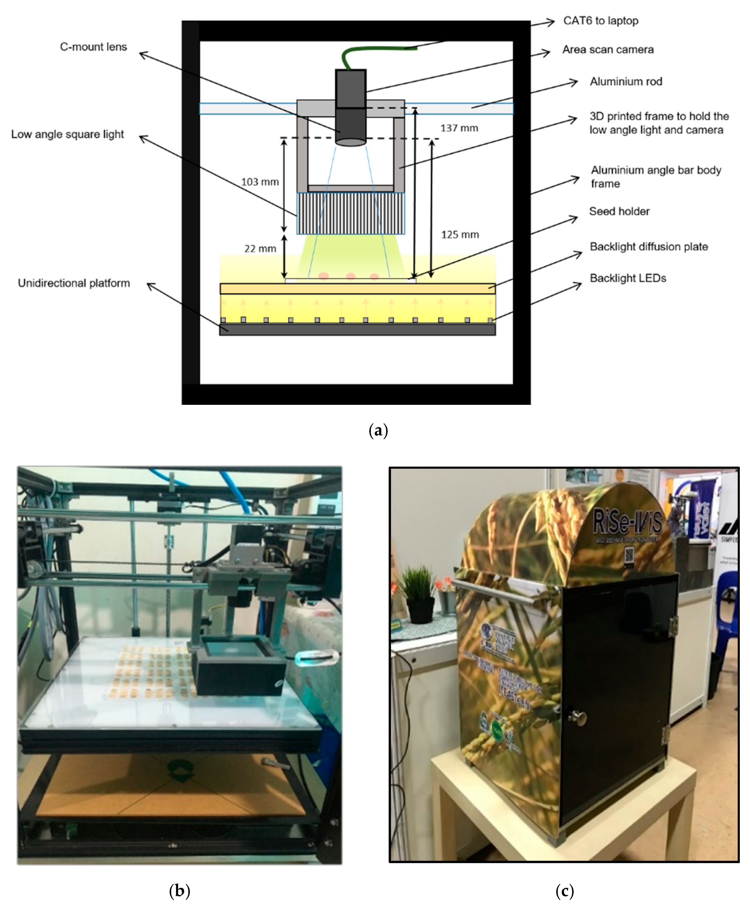
A machine vision system was constructed for the image acquisition of the seed samples. Figure 1 shows the design of the machine vision system for the weedy rice identification. The rice seed kernel images were acquired using an area scan camera (MVCA060-10GC, HIK Vision) equipped with a 6-megapixel resolution, 7.2 mm × 5.4 mm sensor size and 2.4 µm × 2.4 µm pixel size. The CMOS area scan camera was coupled with a 25 mm focal length, f, C-mount lens type. The machine vision used a low-angled diffused square front light (DLW2-60-070-1W-24V) and a high-intensity backlight (BHLX3-00-320x320-X-W-24V) for the uniform illumination of the seed samples. The front light module illuminated the seed sample from above through the emitting diffusion plate from all four directions at an angle of 60° onto the workpiece. Meanwhile, the backlight illumination was modulated from beneath the seed. The combination of the two sources of lighting removed shadows and glare from the seed. Before image acquisition, the camera setting, such as the iris opening, was fully opened. The exposure time was 2000 µs and the balance ratio selector on each plane (Red was 1686, Green was 1024 and Blue was 1690) and the black level at 200 were adjusted and remained constant to ensure the uniformity of the images.

2.3. Image Acquisition

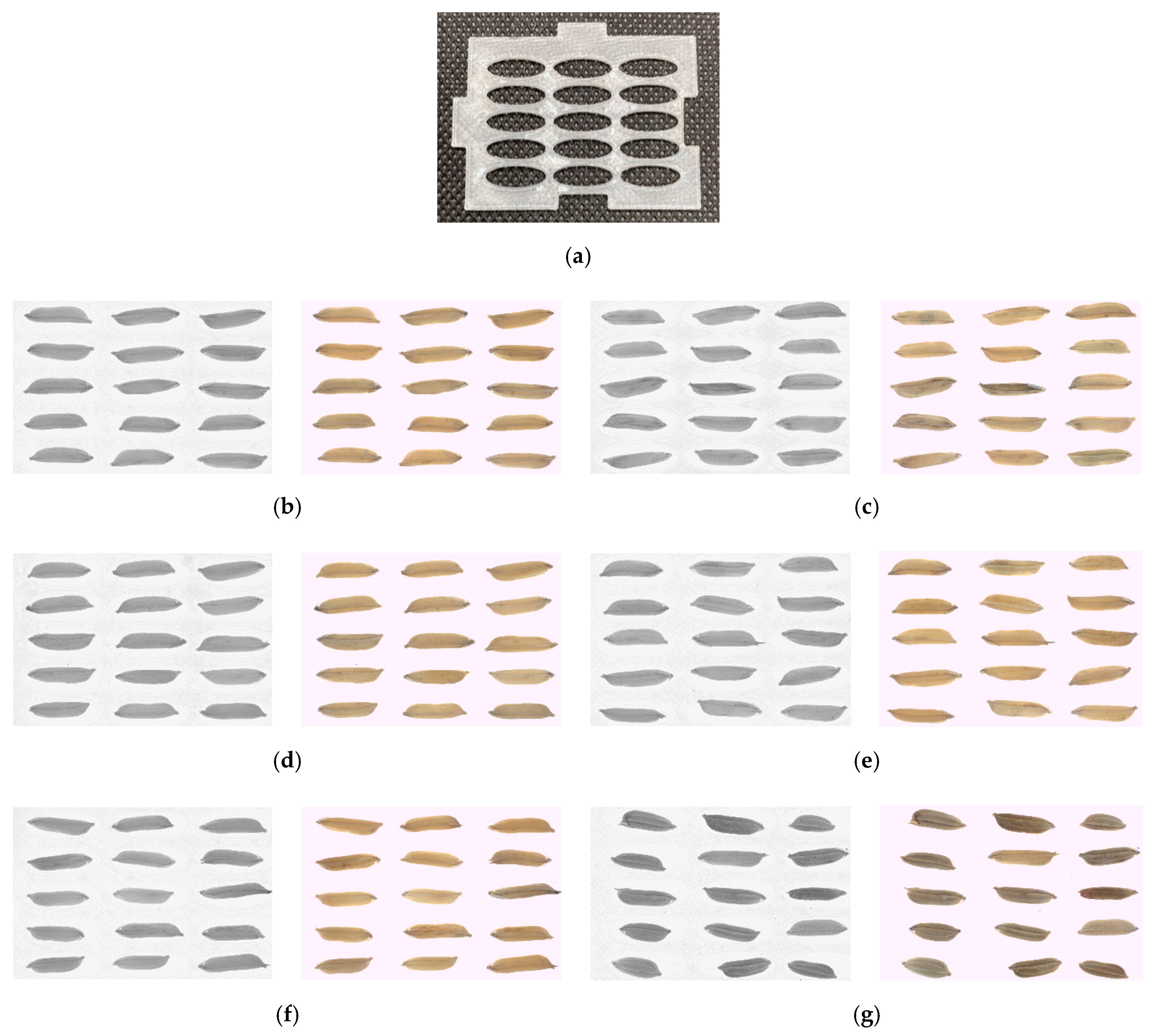
Figure 2 shows the seed holder and the samples of the captured images. The image acquisition process starts by placing the seed samples on a seed holder (Figure 2a) on top of the diffused plate of the backlight illumination model. The seed holder allowed up to 15 seed kernels per image, which fits the field of view offered by the area scan camera. The seed holes were designed with an elliptical shape with a 13 mm length and 4 mm width covering the size of the long grain in the Malaysian varieties. Two types of images were captured, which were RGB and monochrome. Figure 2b–g shows the RGB and monochrome images of the five CR varieties and the weedy rice variants captured on the seed holder. The images captured were then saved in .png format for further image processing and analysis.

2.4. Image Processing and Feature Extraction

LabVIEW 2016 (National Instruments, Austin, TX, USA) software was used to process and extract the RGB and monochrome image features automatically. The 32-bit RGB image processing started with histogram analysis of each Red, Green and Blue colour plane. IMAQ Colour Thresholding removed the white background from the original image and replaced it with an 8-bit greyscale value. Binary conversion replaced the background as 0 or 1 for the sample particles. IMAQ FillHole VI was used as an operation to fill the holes using a pixel value of 1 for any holes found in the sample particle. The IMAQ Particle Filter 3 removed any small particle areas less than the specified lower limit. Image masking utilised IMAQ Masking to complete the image segmentation. For the monochrome image, simple thresholding on the pixel value from 0 to 30,500 (the image format was Mono 12; thus, the pixel value ranged from 0 to 4600) using the IMAQ Threshold VI. The monochrome image was converted to binary, resulting in a 0 for the background and a 1 for the seed kernel. Similarly, the segmentation of the monochrome image was completed by using IMAQ Masking.

The feature extraction used IMAQ Particle analysis to calculate the selected features, such as determining the boundary of the particle sample and the centre of the mass as the reference point of the seed kernel. Three main parameters were extracted from each seed kernel: morphology, colour/greyscale and texture. For the RGB image, a total of 67 features (13 morphology, 24 colour and 30 texture) were extracted. Meanwhile, for the monochrome image, 27 features (13 morphology, 4 greyscale and 10 texture) were extracted. The details for each parameter are as follows.

2.4.1. The Morphological Features

Thirteen morphological features were extracted from the RGB and the monochrome image for the model development. The morphological features were based on the geometric and shape features of the seed kernel. Details of the morphological features are described in

Table 1. The morphological features and their descriptions.

No	Features	Descriptions
1.	Area	Number of pixels in the seed kernel
2.	Perimeter	Length of the pixel boundary of the seed kernel
3.	Convex Hull Perimeter	The length of the smallest convex polygon containing all pixels
4.	Maximum Feret Diameter	The most extended length of the line segment connecting the two endpoints on the seed kernel
5.	Major Axis Length	Length of the major axis of the ellipse that has the same area and same perimeter as the kernel
6.	Minor Axis Length	Length of the minor axis of the ellipse that has the same area and same perimeter as the kernel
7.	Aspect Ratio	Major axis length/Minor axis length
8.	Thinness Ratio	(Seed Perimeter)2/(Seed Area × π)
9.	Ellipse Ratio	Major Axis Length/Minor Axis Length
10.	Hydraulic radius	Disk area/disk perimeter where the disk radius is the distance between a pixel boundary to the centroid of the seed kernel
11.	Angle Orientation	The angle of a line that passes the seed centroid about which the particle has the lowest moment of inertia
12.	Moment XX	The moment on the X direction to the particle centre of mass
13.	Moment YY	The moment on the Y direction to the particle centre of mass

.

2.4.2. The Colour/Greyscale Features

The colour features were extracted from the Red (R), Green (G) and Blue (B) colour planes from the RGB colour model as well as the Hue (H), Saturation (S) and Value (V) colour band from the HSV colour model. The four main colour features extracted from the RGB images were the mean, standard deviation and the minimum and maximum value of each colour plane. Meanwhile, for the monochrome image, a greyscale value range between zero and one was calculated, and four features were extracted from the monochrome image. The features were the mean, variance, standard deviation and mean population of the greyscale value. There were 24 colour features for the RGB images and 4 greyscale features for the monochrome images.

2.4.3. The Textural Features

The Haralick textural features were extracted from the grey level co-occurrence matrix (GLCM). Both image types had a reduction from 0 to 255 values to 8 levels to develop the GLCM array. Ten textural features were computed from the GLCM array on the colour plane of each image. The reduction of 255 grey levels to 8 levels for the GLCM was proven by Majumdar and Jayas [33] to reduce the computational time and increase the grain classification accuracy.

Table 2. The textural features and their description.

No	Parameters	Equation	Description
1.	Mean	${\displaystyle {\displaystyle \sum }_{i,j=0}^{N-1}}i·P_{\left(i,j\right)}$	The estimate of the intensity of all pixels in the relationships that contributed to the GLCM.
2.	Variance	${\displaystyle {\displaystyle \sum }_{i,j=0}^{N-1}}{\left(i-\mu \right)}^2·P_{\left(i,j\right)}$	Measures the heterogeneity and is strongly correlated to the first-order statistical variable such as standard deviation. Variances increase when the grey level values differ from their mean.
3.	Uniformity	${\displaystyle {\displaystyle \sum }_{i,j=0}^{N-1}}{(P_{\left(i,j\right)})}^2$	Measures the textural uniformity that is pixel pair repetitions. Detects disorders in textures and energy reaches a maximum value equal to one.
4.	Entropy	$-{\displaystyle {\displaystyle \sum }_{i,j=0}^{N-1}}(P_{\left(i,j\right)})·log\left(P_{\left(i,j\right)}\right)$	Measures the disorder or complexity of an image. Inversely correlated to energy. The entropy value is large when the image is not texturally uniform. Complex textures tend to have high entropy.
5.	Maximum probability	$Max (P_{\left(i,j\right)})$	The maximum normalised GLCM entry.
6.	Correlation	${\displaystyle {\displaystyle \sum }_{i,j=0}^{N-1}}\frac{\left(i-\mu \right)\left(j-\mu \right)}{{\sigma }^2}·P_{\left(i,j\right)}$	Measures grey level linear dependence between the pixels at the specified position relative to each other. The correlation value is either 1 or -1 for a positive or negative correlated image, respectively. Correlation is NaN for a constant image.
7.	Homogeneity	${\displaystyle {\displaystyle \sum }_{i,j=0}^{N-1}}\frac{P_{\left(i,j\right)}}{1+{\left(i-j\right)}^2}$	Measures image homogeneity as it assumes larger values for smaller grey tone differences in pair elements. It has a maximum value when all image elements are the same. Homogeneity decreases if contrast increases while energy is kept constant.
8.	Contrast	${\displaystyle {\displaystyle \sum }_{i,j=0}^{N-1}} {\left(i-j\right)}^2·P_{\left(i,j\right)}$	Measures the spatial frequency of an image and the difference moment of the GLCM. The difference between the highest and the lowest values of a contiguous set of pixels or measures the number of local variations present in the image.
9.	Cluster Shade	${\displaystyle {\displaystyle \sum }_{i,j=0}^{N-1}} {\left(i+j-2\mu \right)}^3·P_{\left(i,j\right)}$	Measures the skewness of the image. An asymmetric image has a high cluster shade.
10.	Cluster Prominence	${\displaystyle {\displaystyle \sum }_{i,j=0}^{N-1}} {\left(i+j-2\mu \right)}^4·P_{\left(i,j\right)}$	It measures image symmetry. High cluster prominence indicates less symmetry.

shows a description and the formula that [18,33,34] used to calculate the features from the GLCM array. There were 30 textural features for the RGB images and 10 textural features for the monochrome images.

2.5. Classification Model Development

The classification model development was trained using The Classification Learner App available in MATLAB R2020b (Mathworks Inc., Natick, MA, USA). Seven machine learning (ML) classifiers were used, which were mainly the Decision Trees (DT), Discriminant Analysis (DA), Logistic Regression (LR), Naïve Bayes (NB), Support Vector Machine (SVM), Nearest Neighbour (KNN) and Ensemble Classifier (EC). The classification model development utilised all the available options of the ML classifier due to each classifier having different characteristics. Furthermore, the classification performance, especially accuracy, was sensitive to various parameter optimisations for different classifiers [35]. The details of the kernel options available for each of the classifiers are tabulated in

Table 3. The list of ML classifiers, kernel and hyperparameter options used in the classification.

No	Machine Learning	Kernels	Hyperparameter
1.	Decision Tree (DT)	Fine Tree, Medium Tree, Coarse Tree, Optimisable Tree	Maximum number of splits, split criterion, surrogate decision splits
2.	Discriminant Analyses (DA)	Linear Discriminant, Quadratic Discriminants, Optimisable Discriminant	Covariance structure
3.	Logistic Regression (LR)	Logistic Regression	None
4.	Naïve Bayes (NB)	Gaussian Naïve Bayes, Kernel Naïve Bayes, Optimisable Naïve Bayes	Kernel type, support
5.	Support Vector Machine (SVM)	Linear SVM, Quadratic SVM, Cubic SVM, Fine Gaussian SVM, Medium Gaussian SVM, Coarse Gaussian SVM, Optimisable SVM	Kernel function, Box Constraint Level, Kernel Scale, Multi-class method
6.	Nearest Neighbour (KNN)	Fine KNN, Medium KNN, Coarse KNN, Cosine KNN, Cubic KNN, Weighted KNN, Optimisable KNN	Number of neighbours, distance metric, distance weight, standardised data
7.	Ensemble Classifiers (EC)	Boosted Tree, Optimisable Ensemble	Ensemble Method, Learner type, the maximum number of splits, learning rate, number of predictors to sample

. The ML options are tuneable through hyperparameter settings, or users can employ readily available default options. In this study, the initial values used readily available default pre-determined hyperparameters. Each dataset was trained using the available kernels, including the optimisable options.

The optimisable options offered in the ML application trained the dataset using multiple hyperparameters. These hyperparameters were internal parameters of the model and strongly affected its performance once changed. The optimisation from the classification learner apps automatically selected the values of the hyperparameters instead of changing the parameters manually. The optimisation used the Bayesian method and tried different combinations of the hyperparameter values to minimise the classification error and return an optimised model. The classification learner app created a minimum classification error plot during the optimisation of the hyperparameters. The plot updated itself in each iteration (30 iterations) until it found the best point for the hyperparameters to minimise the classification error. Then, the best-optimised model was developed, having the best model classification accuracy. The best model accuracy for each dataset was identified and the confusion matrix of the best model was recorded for further analysis.

2.6. Confusion Matrix

The ML classifier results were analysed using a confusion matrix that explained the accuracy of the developed model. It had four main metrics [36]: the True Positive (TP) to indicate the number of the correct classifications of the WR, and the False Negative (FN) to indicate the number of the incorrect classifications of the WR seed. Meanwhile, the True Negative (TN) shows the number of the correct classifications of the CR, and the False Positive (FP) indicates the number of the incorrect classifications of the CR seed group.

Analyses of the best model were based on the overall performance measures, such as the accuracy and the average correct classification of the classifiers. Accuracy measures the ratio of the accurately estimated samples to the total number of samples. The average correct classification indicated the average percentage of the correctly classified seeds for both groups without bias to any seed group. The formula for the performance measures is shown in Equation (1) to Equation (4):

$$\mathrm{Accuracy}=\frac{\left(TP\right)+\left(TN\right)}{\left(TP\right)+\left(FP\right)+\left(FN\right)+\left(TN\right)}$$

(1)

$$\mathrm{Average}\mathrm{correct}\mathrm{classification}=\frac{Sensitivity+Specificity}{2}$$

(2)

$$\mathrm{Sensitivity}=\frac{\left(TP\right)}{\left(TP\right)+\left(FN\right)}$$

(3)

$$\mathrm{Specificity}=\frac{\left(TN\right)}{\left(TN\right)+\left(FP\right)}$$

(4)

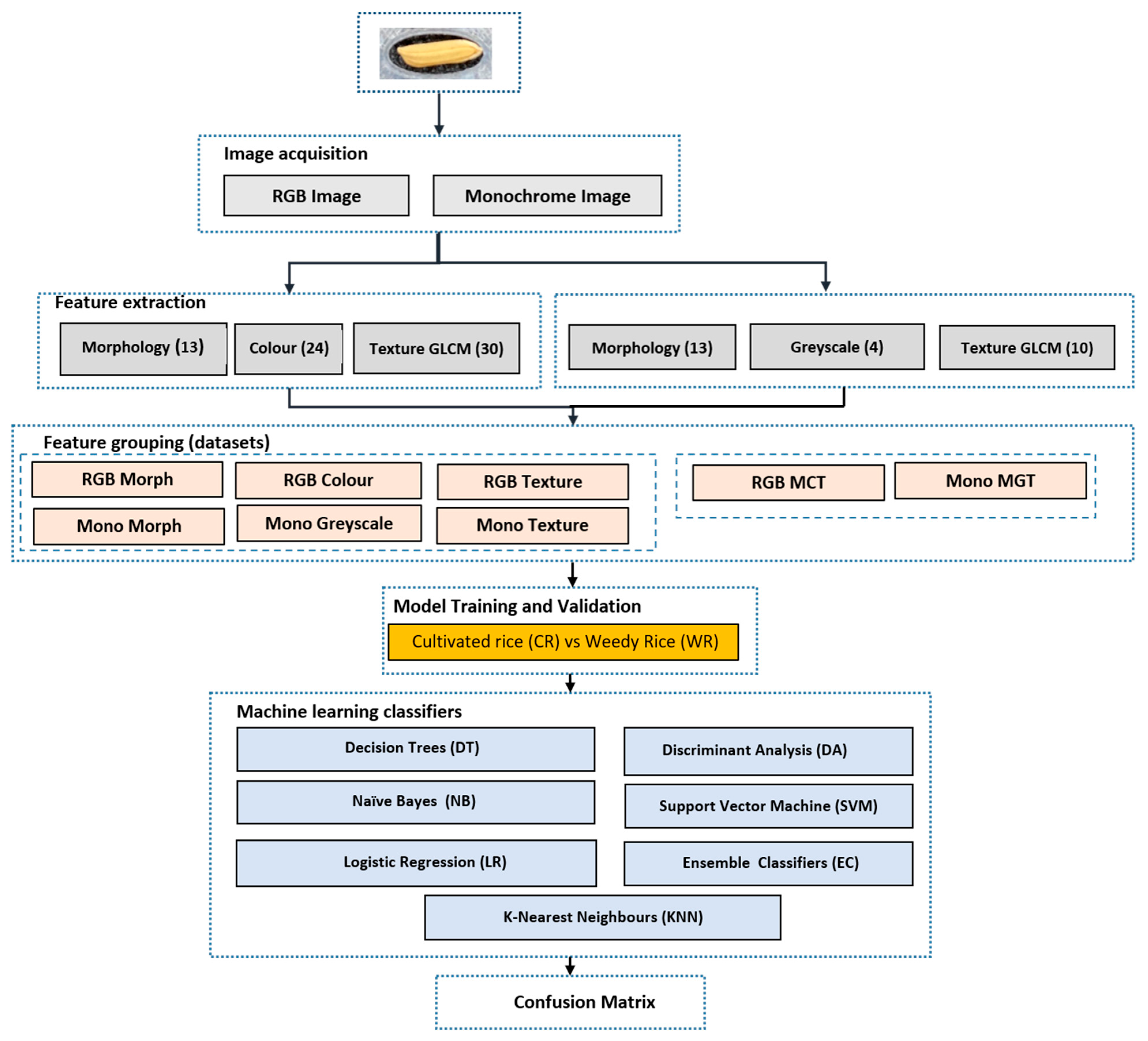
The analysis of this study aimed to determine the best-validated model that emphasised predicting the WR class correctly. Therefore, the best-optimised model was evaluated based on these two main parameters besides the model sensitivity and specificity. The summary of the step-by-step analysis to classify the CR seed and WR seed using ML is presented in the flowchart shown in Figure 3.

3. Results

3.1. Classification Results of the RGB Images

In general, it was observed that the sensitivity was lower than the specificity for all the models in

Table 4. The classification performance of the RGB image datasets for the morphology, colour and texture.

Dataset	ML Classifier	Sensitivity (%)	Specificity (%)	Accuracy (%)	Average Correct Classification (%)
RGB Morph	DT	52.3	99.0	93.9	75.7
	DA	52.3	99.0	93.9	75.7
	NB	61.9 *	92.8	89.4 *	77.4 *
	LR	52.8	99.4	94.4	76.1
	K-NN	47.4	99.5	93.8	73.5
	SVM	52.5	99.7	94.6	76.1
	EC	53.1	99.3	94.2	76.2
RGB Colour	DT	73.7	98.9	96.2	86.3
	DA	81.5	90.3	89.3	85.9
	NB	81.2	91.1	90	86.2
	LR	84.2 **	99.2	97.6 **	91.7 **
	K-NN	72.1	99.4	96.4	85.8
	SVM	83.6	99.2	97.5	91.4
	EC	77.2	99.3	96.9	88.3
RGB Texture	DT	43.4	98.7	92.7	71.1
	DA	58.1	84.6	81.8	71.4
	NB	53	86.5	82.8	69.8
	LR	41.9	99.1	92.9	70.5
	K-NN	37.8	99.2	92.5	68.5
	SVM	38.1	99.2	92.7	68.8
	EC	56.1 ***	98.7	92.8 ***	77.4 ***

* indicates the best model performance for the RGB Morph, ** indicates the best model performance for the RGB Colour and *** indicates the best model performance for the RGB Texture.

. For the RGB Morph, the highest accuracy was attained by the cubic SVM model at 94.6%; however, it had a low sensitivity at 52.5%. In contrast, the optimised NB model had the highest sensitivity (61.9%) which led to 89.4% total accuracy. Both models achieved high specificity, thus influencing each of their total accuracies. Since the classifier performance results did not favour any of the models, the average correct classification was used as another indicator to assess the classifier performance. The optimised NB model had the highest average correct classification at 77.4%. In comparison, the cubic SVM model had an average correct classification of 76.1%, slightly lower than the NB model, while maintaining the highest accuracy. Although the optimised NB model had the lowest accuracy, it also had the highest sensitivity among the other models at 61.9%. This indicates that the optimised NB model, trained using all 13 morphology features, can correctly classify WR compared to the other models.

For the RGB Colour, the LR model achieved the highest accuracy at 97.6% and 91.7% average correct classification. The most increased sensitivity was from the LR model, which obtained 84.2% compared to the lowest value at 72.1% from the weighted KNN model; however, the weighted KNN model had the highest specificity at 99.4%. The LR model had the highest percentage of correctness among all the models at 91.7%. This indicated that the LR model, trained using all 24 colour features, could correctly predict the WR seed at a sensitivity rate of 84.2%, with a misclassification rate of up to 15.8%; simultaneously, the model could predict the CR seed at a high specificity of 98.1%.

The RGB Texture dataset revealed that the highest accuracy was obtained by the LR model at 92.9%; however, the LR model had a moderate average correct classification at 70.5% due to the low sensitivity (41.9%) value. Meanwhile, the highest sensitivity was achieved by the DA model at 58.1%, but the specificity value was low at 84.6%; therefore, this affected the total accuracy of the DA model to be the lowest at 81.8% among the other models. However, the average correct classification of the DA model was slightly higher than the LR model at 71.4%. Even though the DA model had the highest TPR value, the optimised EC model had the highest average correct classification. Therefore, to select the best model for this research objective, the average correct classification was considered.

Comparison between the DA and the optimised EC model revealed that the average correct classification difference between the two models was 6%. Although the WR sensitivity of the EC model was lower by 2%, the specificity was higher by 14.1% from the DA model; thus, the optimised EC model had a higher average correct classification, balancing the ability to predict the two seed groups. Simultaneously, the limitation of 5% differences in the average correct classification, sensitivity and specificity value was decided as a threshold and as the deciding factor should this case arise from the confusion matrix. The 2% difference for the sensitivity difference was acceptable for the EC model, although the DA model had a higher TPR because the average correct classification differences were high at 6%; thus, the best-optimum model using all RGB Texture was the EC model.

Among the three selected models from each of the datasets, the RGB Colour modelled from the LR attained the highest accuracy (97.6%) and average correct classification (91.7%) as compared to the optimised NB for the RGB Morph (89.4% and 77.4%, respectively) and the optimised EC for the RGB Texture (92.8% and 77.4%, respectively); thus, it may be deduced that the colour parameter from the RGB images had a high significance in identifying and separating the WR from the CR seeds.

3.2. Classification Results of the Monochrome Images

Table 5. The classification performance of the Monochrome image datasets for the morphology, greyscale and texture parameters.

Dataset	ML Classifier	Sensitivity (%)	Specificity (%)	Accuracy (%)	Average Correct Classification (%)
Mono Morph	DT	49.1	99.1	93.7	74.1
	DA	50.9	98.8	93.6	74.9
	NB	62.0 *	92.7	89.3	77.4 *
	LR	50.6	99.6	94.2	75.1
	K-NN	46.7	99.4	93.7	73.1
	SVM	52.8	99.6	94.5	76.2
	EC	53.1	99	94	76.1
Mono Grey	DT	64.8	98.3	94.6	81.6
	DA	69.1	98.0	94.8	83.6
	NB	77.8 **	95.0	93.2	86.4 **
	LR	64.9	98.7	95	81.8
	K-NN	67.8	98.5	95.2	83.2
	SVM	52.8	99.6	95.1	81.6
	EC	53.1	99	94.9	82.1
Mono Texture	DT	18.3	99.2	90.5	58.8
	DA	51.0 ***	86.7	82.8	68.9 ***
	NB	49.4	86.8	82.8	68.1
	LR	18.2	99.4	90.6	58.8
	K-NN	23.4	98.8	90.6	61.1
	SVM	18.2	99.4	90.5	58.8
	EC	20.9	99.0	90.5	60

* indicates the best model performance for the Mono Morph, ** indicates the best model performance for the Mono Grey and *** indicates the best model performance for the Mono Texture.

shows the classification performance of the Monochrome image trained using the seven ML classifiers. The Mono Morph classification performance had the highest accuracy by the cubic SVM model at 94.5%; however, the average correct classification of the cubic SVM model was moderate at 76.2% compared to the other classifiers. The optimised NB model achieved the highest average correct classification at 77.4% by having the highest sensitivity at 62% compared to the cubic SVM model; thus, the NB model was selected as the best model to classify the WR and CR seed for the Mono Morph dataset.

The Mono Grey classification performance, which employed four features, achieved the highest accuracy at 95.2% through the optimised K-NN model; meanwhile, the highest sensitivity was obtained by the optimised NB model at 77.8%, and its respective specificity was 95%, slightly lower than the KNN model. The values led the accuracy of the optimised NB model to 93.2%, the lowest among the other models; however, it had the highest average correct classification at 86.4%. Therefore, the optimised NB model was the best model performance for the Mono Grey dataset.

For the Mono Texture dataset, the LR and the optimised KNN model obtained the highest accuracy at 90.6%; however, the sensitivity was low at 18.2% and 23.4%, respectively. Meanwhile, the specificity values were high at 99.4% and 98.8%, respectively. The average correct classification of the LR and KNN model was moderate at 58.8% and 61.1%, respectively, influenced by the low sensitivity but high specificity; meanwhile, the DA model achieved the highest sensitivity at 51%, but had the lowest accuracy at 82.8% among the other models. However, the average correct classification of the DA modes was the highest at 68.9%; therefore, the optimised DA model was selected as the best optimum model for the Mono Texture dataset.

A comparison among the parameters extracted from the monochrome image revealed that the best-optimum model was the Mono Grey, which achieved the highest sensitivity (77.8%), specificity (95%), accuracy (93.2%) and average correct classification model at 86.4%. This indicated that the greyscale value of the monochrome image had a significant impact on the WR identification compared to the morphology and texture parameters.

3.3. Classification Results of the Combined Parameters

Table 6. The classification performance of the combined parameters of the RGB and Monochrome image datasets for the morphology, greyscale and texture parameters.

Dataset	ML Classifier	Sensitivity (%)	Specificity (%)	Accuracy (%)	Average Correct Classification (%)
RGB MCT	DT	79.1	99.1	97	89.1
	DA	80.1	96.6	94.8	88.4
	NB	79.6	95.6	93.9	87.6
	LR	85.3 *	99.5	97.9	92.4 *
	K-NN	69.7	99.7	96.8	84.7
	SVM	83.9	99.6	97.9	91.8
	EC	81.3	99.5	97.6	90.4
Mono MGT	DT	74.5	98.9	96.3	86.7
	DA	78.5	96.1	94.2	87.3
	NB	78.5	95.5	93.7	87
	LR	76.4	99.3	96.8	87.9
	K-NN	68.6	99.6	96.2	84.1
	SVM	78.9 **	99.5	97.3	89.2 **
	EC	77.2	99.3	96.9	88.3

* indicates the best model performance for the RGB MCT and ** indicates the best model performance for the Mono MGT.

shows the classification performance of the combined parameters respective to each image type. For the RGB MCT dataset, the highest accuracy was 97.9%, where the LR and optimised SVM models shared the same accuracy. The optimised SVM, which attained 97.9% accuracy, had 83.9% sensitivity and 99.6% specificity. The LR model had a slightly higher sensitivity at 85.3% than the optimised SVM and the highest average correct classification (92.4%) among the other models; therefore, the LR model was selected as the best-optimum model for the RGB MCT dataset.

For the Mono MGT dataset, the highest accuracy and sensitivity were obtained by the optimised SVM model at 97.3% and 78.9%. This led the optimised SVM model to attain the highest average correct classification at 89.2%, among the other classifiers, and was selected as the best model for the Mono MGT dataset. The optimised SVM model used a linear kernel function with an optimised box constraint at 55.54 after the 10th iteration of finding the best point hyperparameters to minimise the classification error. A comparison among the two models revealed that the RGB MCT model had better prediction models (sensitivity 85.3%) than the Mono MGT (sensitivity 78.9%) model.

4. Discussion

For the single-parameter classification model, it was found that either using a monochrome or RGB image did not influence the performance of the classification of the morphological features. Meanwhile, both the RGB Colour and Mono Grey datasets had higher sensitivity than the morphological or textural features. Among the two datasets, the colour parameter had better sensitivity at 84.2% in differentiating the WR and CR seeds. Nevertheless, the textural features had the lowest sensitivity either using the RGB or monochrome image.

The WR detection (sensitivity) increased to 85.3% when modelled using the combination of the three parameters based on the RGB MCT dataset, which thus led to 92.4% average correct classification and 97.9% accuracy. The addition of the morphological and textural features proved to improve the sensitivity in WR detection. Adding more features helped to improve accuracy and sensitivity, similar to the work of [12,37]. Therefore, the RGB MCT model, which utilised all the 67 features (13 Morphology + 24 Colour + 30 Texture) using the LR model, was selected as the best optimum model for WR classification. Furthermore, Sudianto et al. [31] proved that the WR seed had darker pigmented hull colours ranging from brown, black and brown striped/furrows as compared to the matured cultivated rice seed, which thus influenced the classification model performance.

The previous work on weedy rice seed classification by Aznan et al. [32] used Discriminant Analysis to develop a model with an accuracy of 96% to classify the cultivated rice seed MR263 and a weedy rice variant. However, the developed model only utilised the morphological features of the seeds and tested against one variety of the cultivated seeds compared to the present study, which used five popular rice seed varieties to develop a more robust model.

Many researchers have reported total accuracy [19,21,22,37] as the primary indicator to overview the overall performance of an ML classifier. This is due to the simplicity of the accuracy of the measurement that provides the percentage of the correctly classified classes from the total samples. Nevertheless, accuracy is a biased meter as it does not compensate for successes due to mere chance [38] and is often a sensitive metric for measuring performance [39], especially for an imbalanced dataset [36]. Usually, the accuracy is influenced by the higher success rate in one class. Thus, this study proposed the average correct classification as another performance metric that influences the selection of the best model that best describes both classes in a balanced manner. Furthermore, the emphasis on the sensitivity of the WR class is the focus of the present study, where having a false negative is considered undesirable rather than a false positive.

The novelty of this work focuses on finding the best classification model to differentiate between weedy rice and cultivated rice seeds using machine vision technology in the rice seed industry. It is essential to find a methodology to separate the weedy rice from the cultivated rice seed as it is beneficial to the farmers in producing a high-quality seed. It also reduces the number of weedy rice seeds to go back into the farmland, thus reducing the upcoming weedy rice plants during the planting season.

5. Conclusions

This study has shown that a machine vision technique is able to differentiate weedy rice variants from five cultivated rice seeds. The classification performance used input features from the RGB image which outperformed the monochrome version. Furthermore, the combination of the morphology, colour and texture parameters from the RGB image provided better sensitivity and average correct classification than the performance of the single parameter. The best performance for WR detection was achieved by combining the 13 morphology, 27 colour and 30 texture parameters trained using the LR model and achieved 85.3% sensitivity, 99.5% specificity, 97.9% accuracy and 92.4% average correct classification. It is important to evaluate other performance tools, especially the sensitivity of the WR class, and further decide the best optimum model using the accuracy and average correct classification. Further studies are required to improve the classification performance by optimising the number of features to reduce the computational requirements.