1. Introduction
Taiwan is mainly covered by mountainous terrains and forests, and it ranks among the 20 most densely populated places in the world. Hence, there are very limited lands available for agricultural farming. Other factors, such as the aging agricultural population and climate change, make the cost of agricultural operations much higher than in other countries. Moreover, because of the frequent occurrence of typhoons and the impact of extreme weather in recent years, the income of farmers is not as stable as in other industries. In order to ensure benefits for farmers, especially in terms of income security, one of the important primary tasks of the government’s agricultural department is to accurately forecast the crop yield production in order to stabilize the production and sales of agriculture products.
Since 2008, the Agricultural Research Institute in Taiwan has started to use aerial photos and hyperspectral satellite images for crop cultivation area estimation [
1,
2,
3]. Some of its achievements have been recognized by the government’s agriculture office, under the Council of Agriculture, Taiwan, and the methods were adopted to collect reference data. However, these agricultural surveys were conducted manually or semiautomatically. This study develops an automated crop growth detection method that integrates artificial intelligence (AI) with the geographic information platform that was built by the Council of Agriculture in order to provide a faster, more accurate, and labor-saving prediction of the crop yield production.
Cabbage is an important vegetable in Taiwan, and it is usually grown and harvested during the intercropping period in the fall and winter. Because the growth period of cabbage is short, and growing cabbage is fairly easy, cabbage is always selected as one of the intercrops. Nevertheless, the imbalance between cabbage production and sales remains a perennial problem. When overproduction occurs, the market price drops dramatically, and, on the other hand, if crops are devastated by typhoons, the cabbage prices rise substantially. Therefore, being able to accurately estimate the area of the cabbage field and predict the cabbage yield are important tasks for the government agriculture department in order to stabilize cabbage prices. The total area of cabbage fields can be estimated by the monthly number of seedlings. Currently, the Agriculture and Food Agency in Taiwan collects the numbers of seedlings every ten days, with a numerical error less than 10%. Since cabbages will be ready to harvest at around 70 days after planting, the monthly cabbage yield can also be obtained. However, the price-stabilization policy might not be efficiently implemented since the agricultural survey by the Agriculture and Food Agency does not include the cabbage cultivation locations. The Taiwan Agricultural Research Institute, on the other hand, uses satellite photos for agricultural interpretations. Basically, after 40 days of growth, the cultivation locations of cabbages can be inferred from the satellite photos and, on the basis of the calculated harvest areas, the cabbage yield can be predicted. Although the method that has been adopted by the Taiwan Agricultural Research Institute is able to capture the geographic locations, it can only be performed during the early heading stage (i.e., the mid-to-late growth stages). As a result, the cost of price stabilization has increased significantly.
In this study, we used the abovementioned ground-truth data of the collected cabbages, multitemporal multispectral satellite image information with deep learning, and GBDT for the loopback analysis, in order to train a model that can predict the full cycle of the cabbage growth days. If properly implemented, this model can help agricultural units to estimate the harvest areas of cabbage in the early stage, and to deal with the problem of imbalance in production and sales.
This paper consists of six sections.
Section 1 introduces the motivation and the problem statement.
Section 2 presents the background and a review of the related literature and studies, including the production and sales challenges of cabbages, studies based on multitemporal satellite images, and research on spectral satellite image analysis for feature recognition.
Section 3 describes how to collect ground-truth data, and how to obtain the corresponding satellite spectral data. Moreover, the gradient boosting decision tree (GBDT) algorithm for data mining is stated.
Section 4 reports the experiment results, including the assembly of the ground-truth data and the satellite imagery data, the selection of the image features, the GBDT validation results, and the programming language and software that are adopted in this paper.
Section 4 and
Section 5 provide the results and discussions, and the conclusions, respectively.
2. Materials and Methods
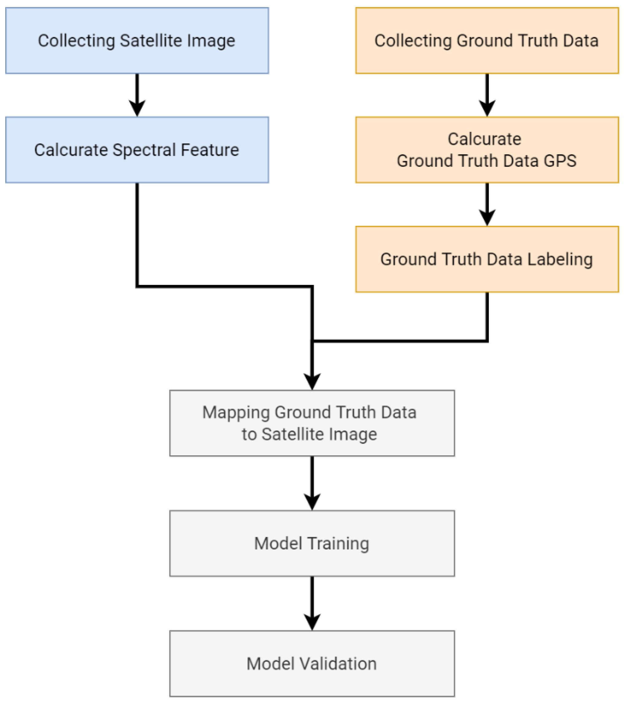
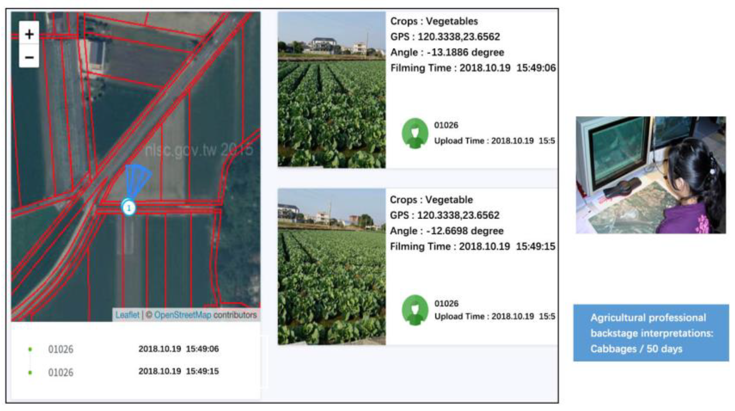
This study aims to create an AI-based model that can interpret satellite images and that can predict the growth stages, or the days of growth, of cabbage. First, ground-truth data, with accurate records of the areas and the values of the land and information on the landholders, must be gathered. The traditional process of ground-truth data collection involves the information and photographs that are collected on location, and the validation of the cadastral data. In order to make it easier to conduct surveys, this study develops an APP that can obtain the cadastral data at the time of the image acquisition. Next, agricultural professionals can interpret the growth stages of the crops according to these ground-truth data. After the interpretations of the agricultural professionals and the cadastral data labelling, these ground-truth data can be used as the learning goals of the data mining techniques on the satellite images in this study.
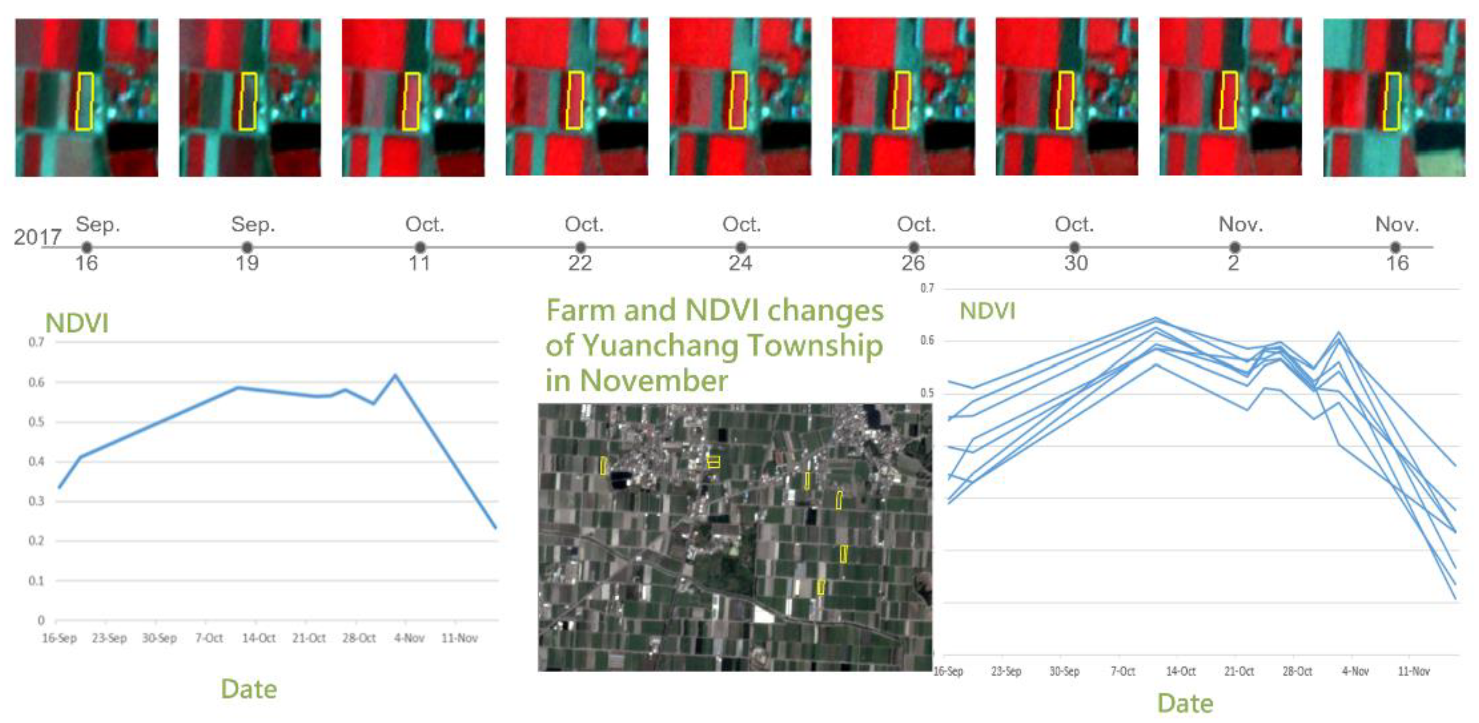
On the basis of the cadastral data of the grouth-truth data, the satellite images on the day of the image acquistion, and the growth stages that were interpreted by professionals, as
Figure 1 shows, the APP accessed the satellite images of the full growth stages before and after the photos were taken as the raw data for interpretation and anticipation.
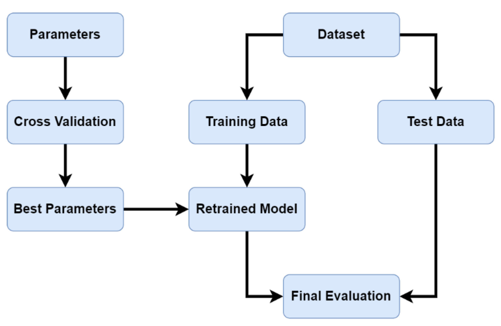
Data mining is a technology that is used for full data analysis, and it mainly involves the process of finding useful information in big data, the results of which are usually used to make various decisions. The cleaned data will be divided into training data and test data. Training data is used to train a model that can identify or make this decision, and the model defines its parameters, and it is then continuously trained to find the best parameters. Test data is used to validate the final trained model for final validation in order to ensure that the model is not recognized by only the training data. The overall process is shown in
Figure 2.
2.1. Ground-Truth Data Collection
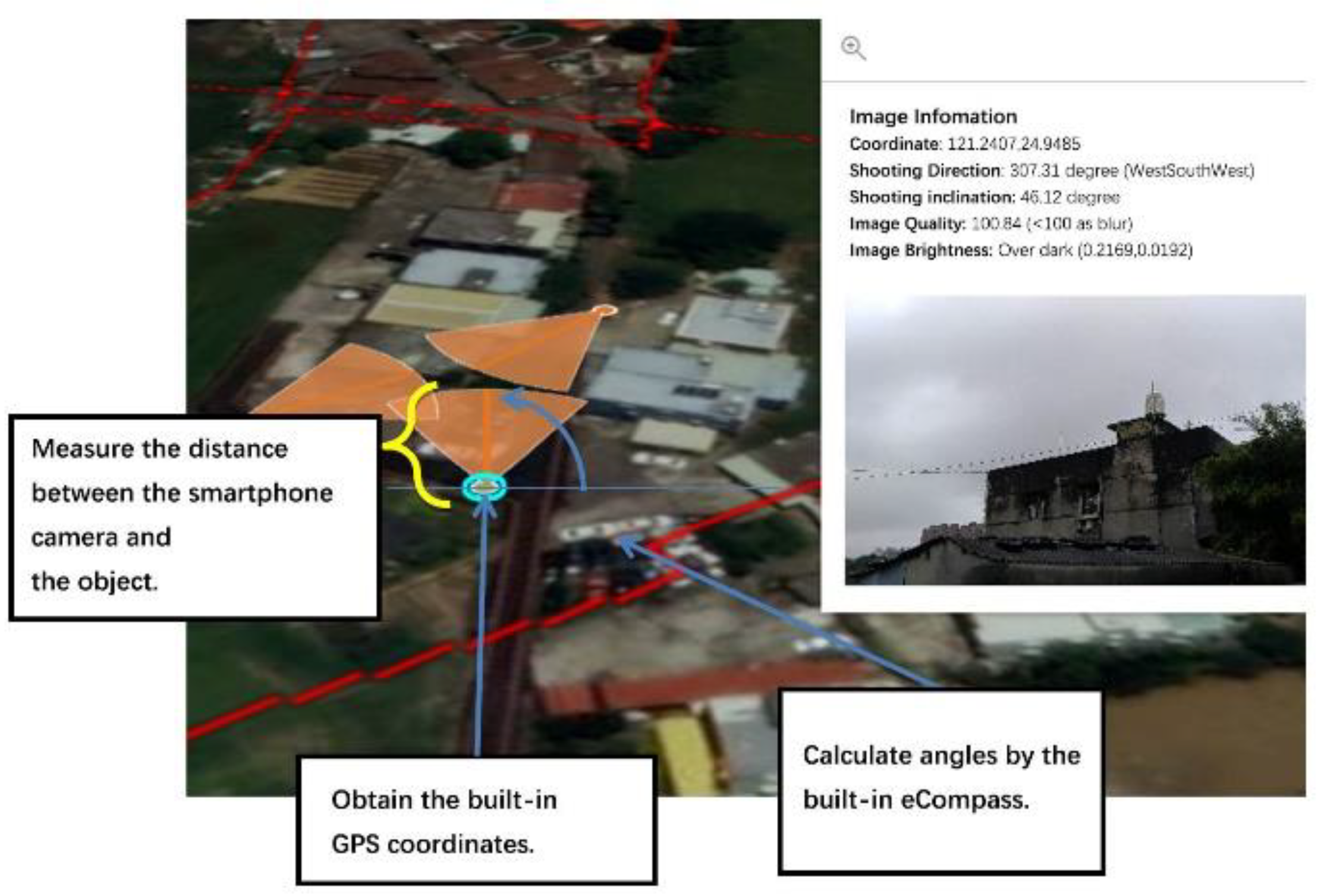
The development of the agricultural survey APP allows users to easily photograph ground objects without additional equipment or special photography techniques. The key point for ground-truth data collection is to take photos that can accurately reveal the location of an object (i.e., the distance between the smartphone camera and the target object) (see
Figure 3.).
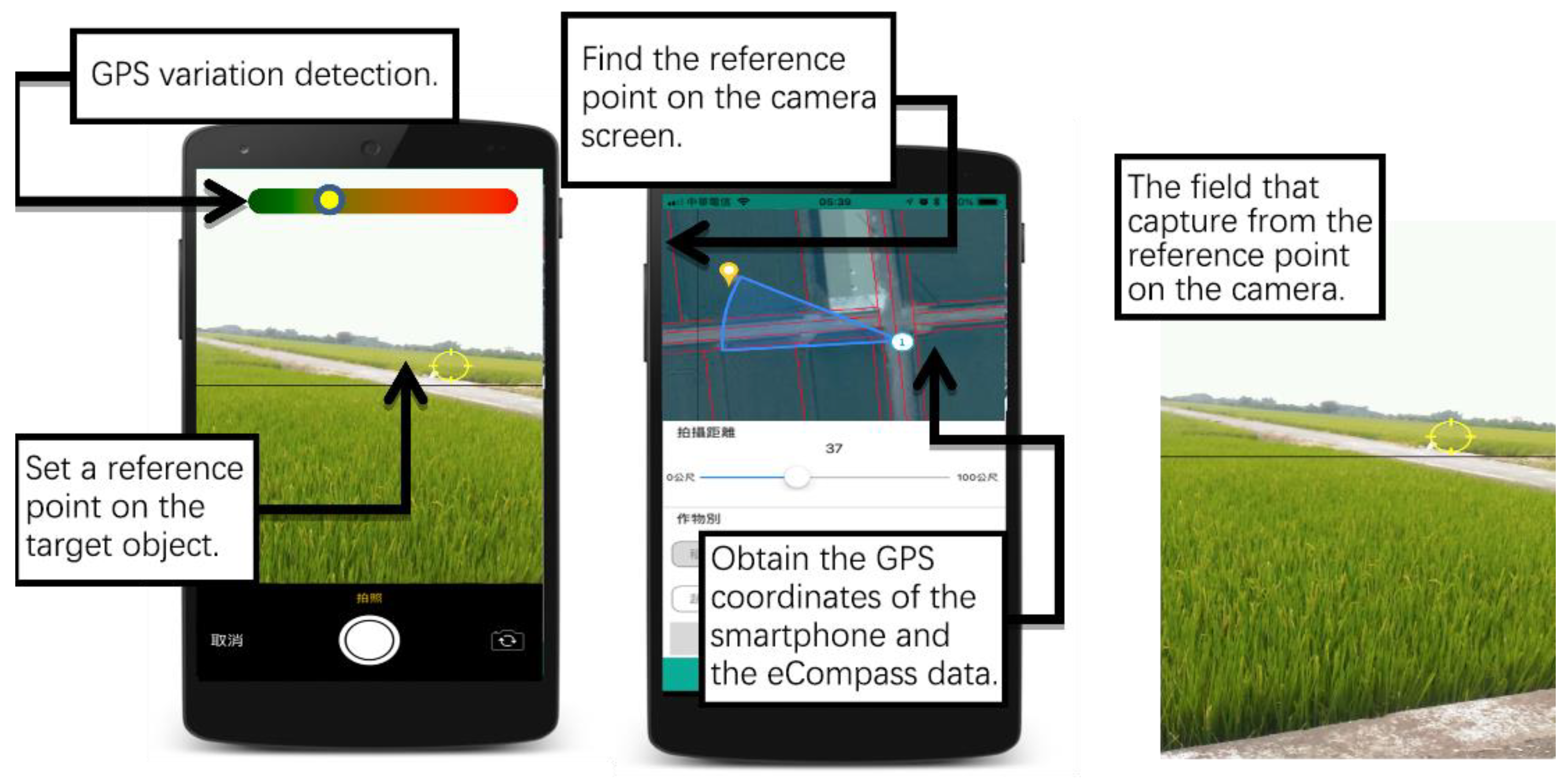
Although smartphone cameras have built-in GPS systems to find the coordinates of the phone, the purpose of agricultural surveys is to find the cadastral data of the crop cultivation area. Therefore, the proposed agricultural survey APP adds a reference point on the camera screen for users to set on the target object. Since GPS results may differ between the smartphones of different brands, some brands of cameras are made of non-single lenses, and the target distance can be calculated by using the function of the camera. However, if the phone has only a single lens, it is impossible to calculate the target distance directly. Therefore, in order to avoid brand differences, some adjustments were made, and the proposed APP has a function to detect variations in the GPS. As shown in
Figure 4, it is only when variations in the GPS are small that the user can take photos successfully.
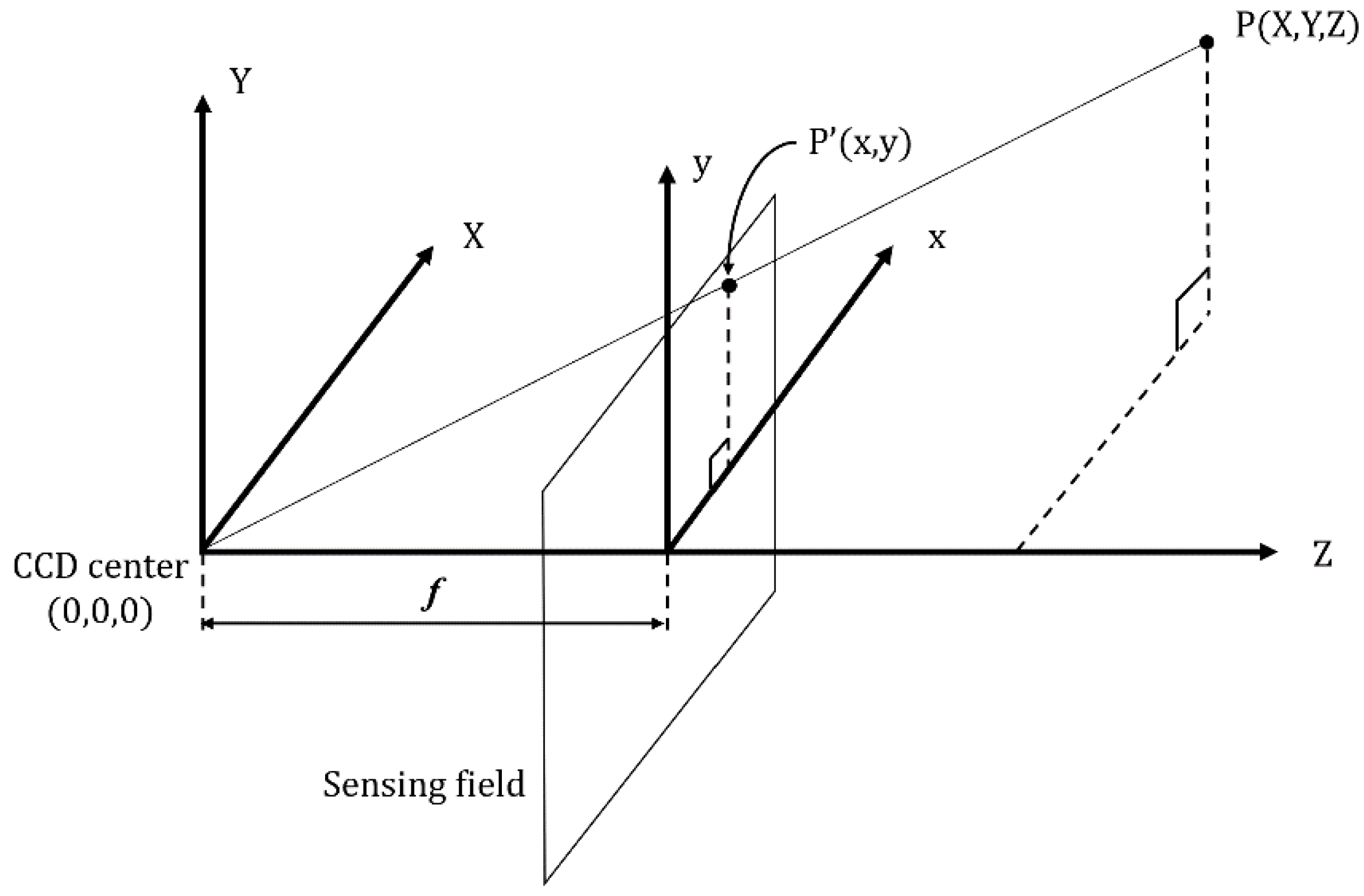
As depicted in
Figure 5, this study assumes that the coordinates of the CCD center are (0,0,0); that the coordinates of the target object (P) are (
X,
Y,
Z); that the coordinates of the object in the image plane is (
x,
y); and that the focal length is
f (Equation (1)):
Moreover, the study assumes that the coordinates of the object (P) in the local coordinate system are
; that the coordinates of the CCD center are
; and the matrix is rotated in order to obtain the coordinates of the object (P) (Equations (2) and (3)):
The abovementioned equations can lead to the following two collinearity equations (Equation (4)):
With the coordinates of the smartphone at the time of the image acquisition and the angle of elevation, the proposed APP can find the coordinates of the CCD center. Next, the camera with a 55AE lens must be set at a height of 1.5 m in order to calculate the coordinates of the object .
2.2. Satellite Image Processing
According to the cadastral data of the grouth-truth data (the date of the image acquistion and the growth stages that were interpreted by the agricultural professionals) the proposed APP retrieves the needed satellite images of the full growth stages. This study uses the multispectral SkySat satellite imagery that is owned by the U.S. company, Planet, which records the red, green, blue, and near-infrared (NIR) light that is reflected off the ground.
The satellite images were postprocessed with Haralick Texture [
4,
5], which was introduced by Haralick in 1973. Haralick Texture can express the quantitative value of the surface material of an object, and, when it is necessary to compare the touch, texture, or pattern of different materials, this method can express the difference value in their features. Thus, it was used to extract the features of the satellite image as one of the parameters for the training. The SEaTH algorithm [
6] was also used to find the most suitable threshold value for each band of the satellite spectrum as a feature to recognize cabbage.
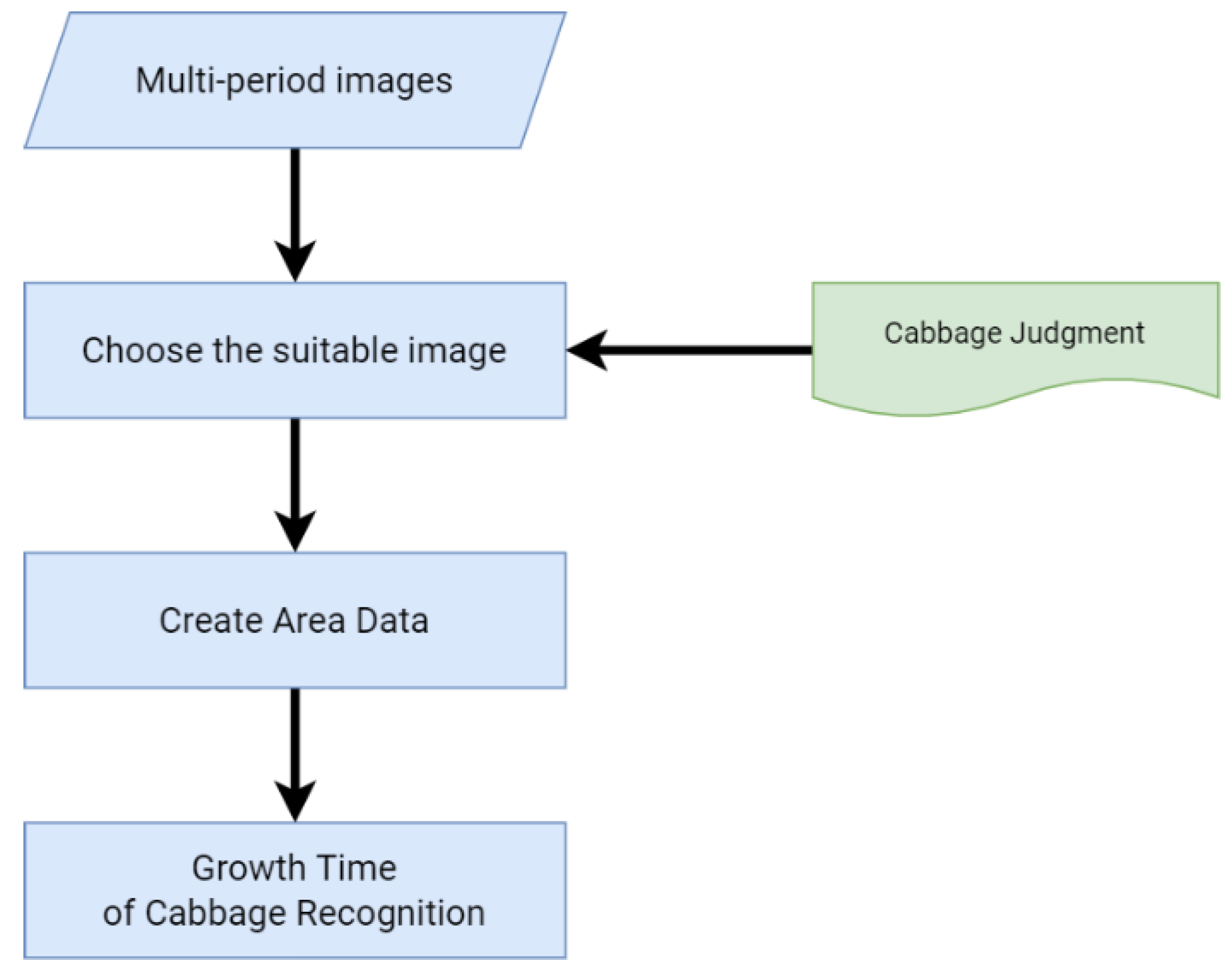
The processed data were also classified into growers by using by differenced image classification [
7,
8] (shown on
Figure 6) and the photographic images in order to ensure that the satellite images could effectively distinguish objects that were not otherwise apparent in the images of the single growth days. For example, on the basis of the normalized difference vegetation index (NDVI) and the spectral reflection curves of the cabbage on different growth days, several satellite images of different growth days can be selected in the same area, and the image of the growth time of the cabbage can be used as the reference point to calculate the growth days of the cabbage in the satellite images of the same area. The difference values of the different growth days for the influence characteristics of the same area can be used to highlight the differences in the different growth periods of the cabbage.
2.3. Data Mining Method: Gradient Boosting Decision Tree (GBDT)
Decision trees (DTs) are used as a basic machine learning method for classification and regression [
9]. DTs with visual explainability speed up the processing time, but overfitting can easily occur. Although pruning helps to prevent overfitting, its efficacy is not significant. Boosting is a method that is used in classification to equally weight all of the training examples, such as by increasing the weight of incorrectly classified examples, and by decreasing the weight of correctly classified examples. The boosting method trains multiple classifiers in linear combinations so as to improve their performance.
The gradient boosting algorithm is an ensemble machine learning method that combines many different algorithms in the framework, and every model is created at the gradient descent direction of the loss function for the model performance evaluation [
10]. Generally, the smaller values of the loss function represent the better performance of the model. Minimizing the loss function simultaneously boosts the performance of the model. Therefore, the optimal method is to decrease the gradient of the loss function so as to improve the model performance.
2.3.1. Tree Ensemble Methods
Tree ensemble methods, including GBM, GBDT, and random forests, are commonly used, and particularly for classification and regression problems. Tree ensemble methods comprise several features:
Tree ensemble methods do not reduce or change the input variables. It is not necessary to standardize the input variables;
Tree ensemble methods allow users to understand the correlations between variables;
Tree ensemble methods can be used in multiple research fields for quantization.
GBDT, which is the model that is based on tree ensembles, is a technique that continuously wins Kaggle and other data analysis competitions, and it has also been extensively used in both academia and industry. GBDT integrates the gradient boosting algorithm with the decision tree algorithm for deep learning. Since one single decision tree cannot satisfy practical applications, GBDT creates many CART-based decision trees, and the sum of the functions (
) on each decision tree is used to reflect the result of each attribute (Equation (5)):
The definitions of the variables are as follows: K is the number of decision trees; f is the functions in the function space, ; and is all possible CART ensembles.
Generally, the way to optimize supervised learning is to train the sum of Loss + Regularization (Equations (6)–(8)) to the minimum. The loss function (
) must be trained first before regularization (
) in order to simplify the branches and the depths of the decision trees, or to adjust the weight for a second derivative:
The optimization of GBDT can be achieved by using the following heuristic method (Equation (9)):
Determine the next step according to the computational results: train the model by using the loss function to minimize errors;
Cut off redundant branches: standardize the branches of the decision trees to simplify the complexity of the trees;
Explore the deepest decision tree: limit the expansion of the functions;
Balance the extensiveness of the leaf nodes: standardize the weight of the second- derivative leaf nodes.
2.3.2. Gradient Boosting Machine Learning Techniques
GBDT first fixes what has been learned, and it determines the function of a tree whenever a new tree is added. In Equation (10),
is the
t-th step:
As Equation (11) shows, the decision tree that learned in the t-th step determines the tree to add (
) according to the minimum optimization objective:
2.3.3. Optimization Objective
To achieve the goal of square loss = 0,
- 2.
Regularization for Decision Trees
According to Equation (15), the tree is defined as a set of vectors, in which
is the number of leaves, and
is the second regularization of the leaf weight:
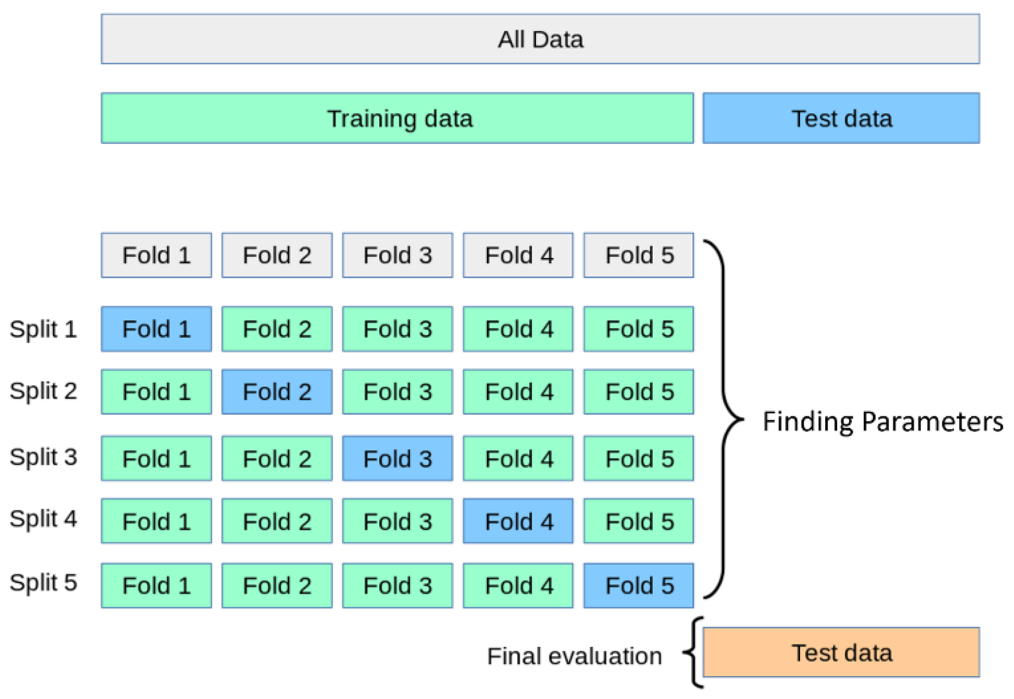
2.3.4. K-Fold Cross Validation for Data Mining
The K-fold cross-validation method splits the training dataset into k subsamples, among which one subsample is used as the test data for the model validation, while the rest of the k-1 subsamples are used as training data. The k-fold cross-validation process is repeated k times, with each of the k subsamples used exactly once for validation. The k results from the folds are averaged or combined in order to generate a single estimation (
Figure 7).
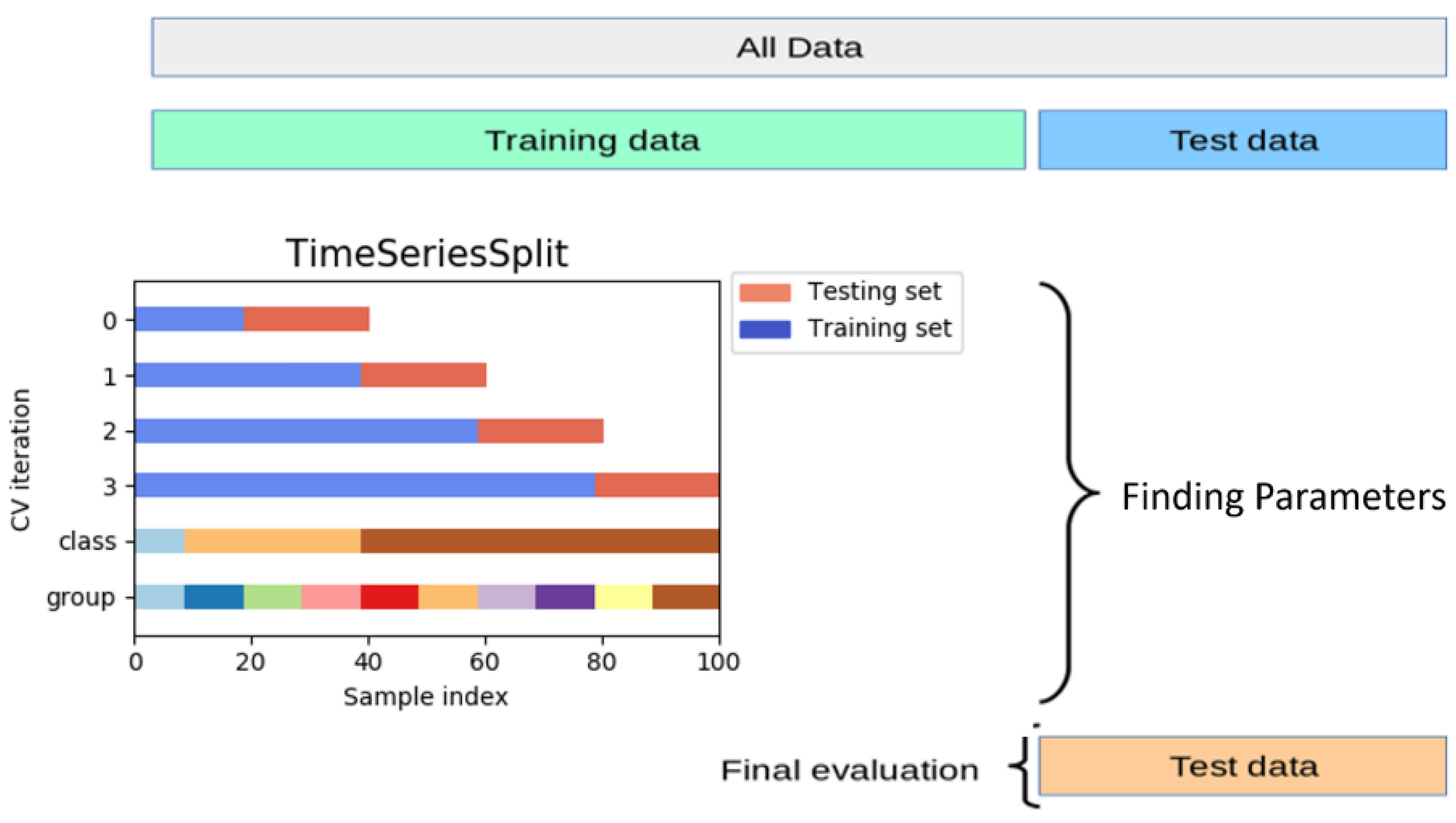
Since our dataset is recorded over consistent intervals of time, the data are arranged in chronological order for the cross validation. The growth days of the cabbages can then be predicted according to the historical data collected, as shown in
Figure 8.
2.3.5. Model Validation
Validation of Regression Models: the mean absolute error (
MAE) is the average absolute difference between the observed values and the calculated values. Since absolute errors in replicated measurements of the same physical quantity may differ, we averaged the absolute value of the errors in order to obtain the
MAE. Compared with the mean error, the
MAE is an absolute error measure that is used to prevent the positive and negative deviations from canceling one another. Therefore, the
MAE can better reflect the real situation of the error of prediction (Equation (16)):
Validation of Classification Models: a confusion matrix is created on the basis of the values of the real target attributes and the predicted values in order to compute the classification metrics, including the precision, the recall and the F-measure.
Figure 9 shows the abovementioned steps and the flowchart of the methodology.
3. Results
3.1. Ground-Truth Data and Satellite Imagery Data Collection
3.1.1. Ground-Truth Data
During the period from 15 December 2018 to 11 February 2019, the field survey APP captured 735 ground-truth data records of the cabbage cultivation areas in Yunlin County, and agricultural professionals examined the records in order to interpret the cabbage growth stages, as shown in
Figure 10 and
Figure 11.
3.1.2. Satellite Imagery Data
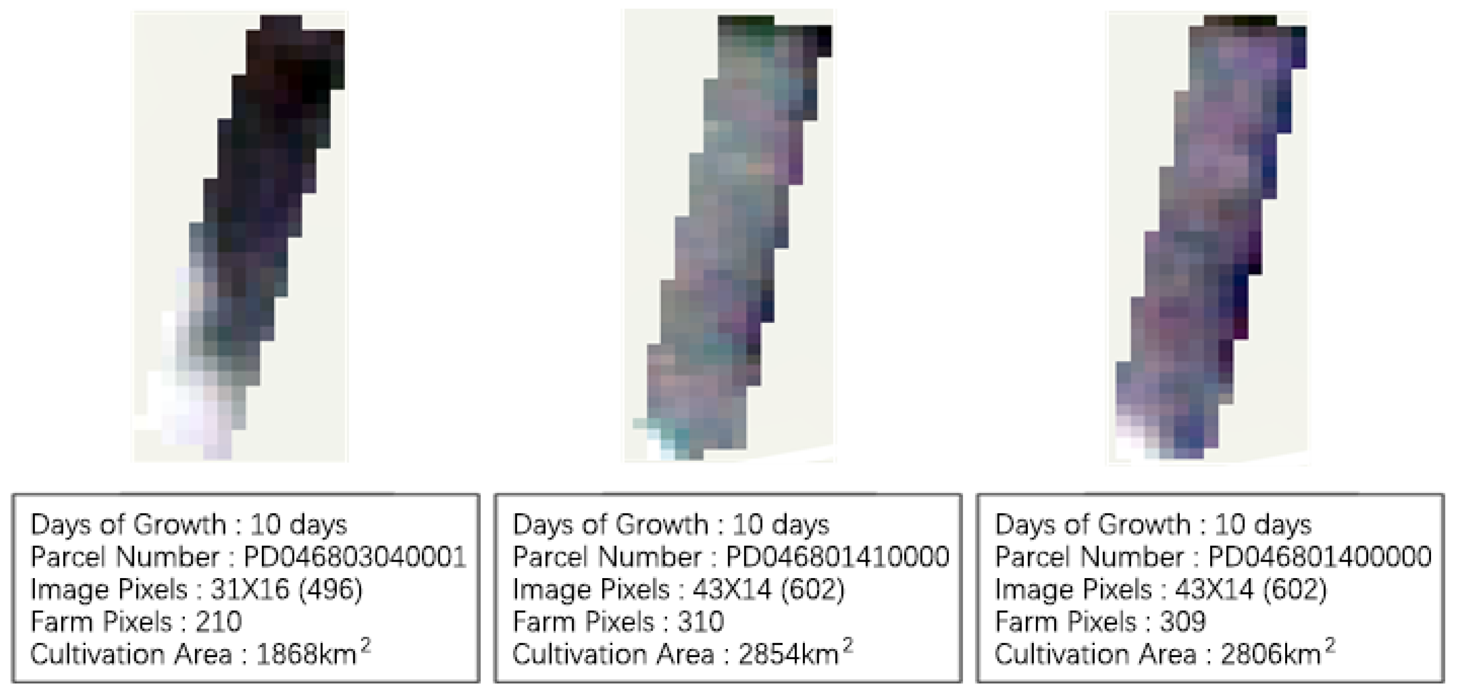
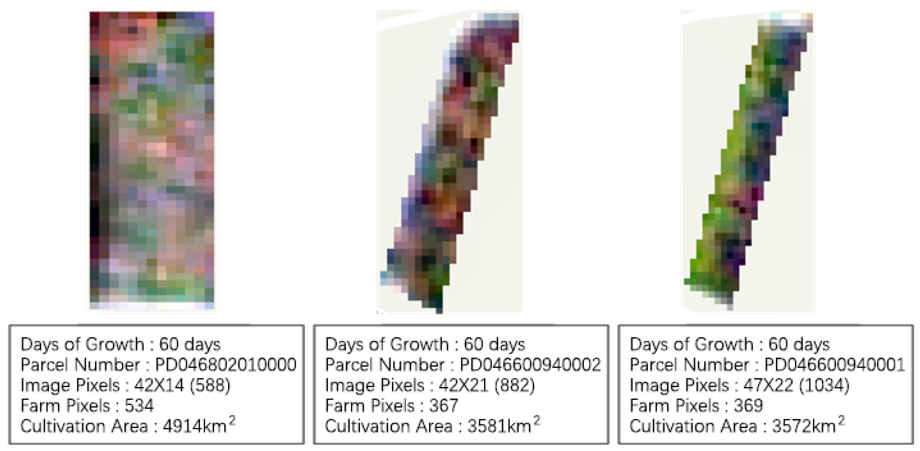
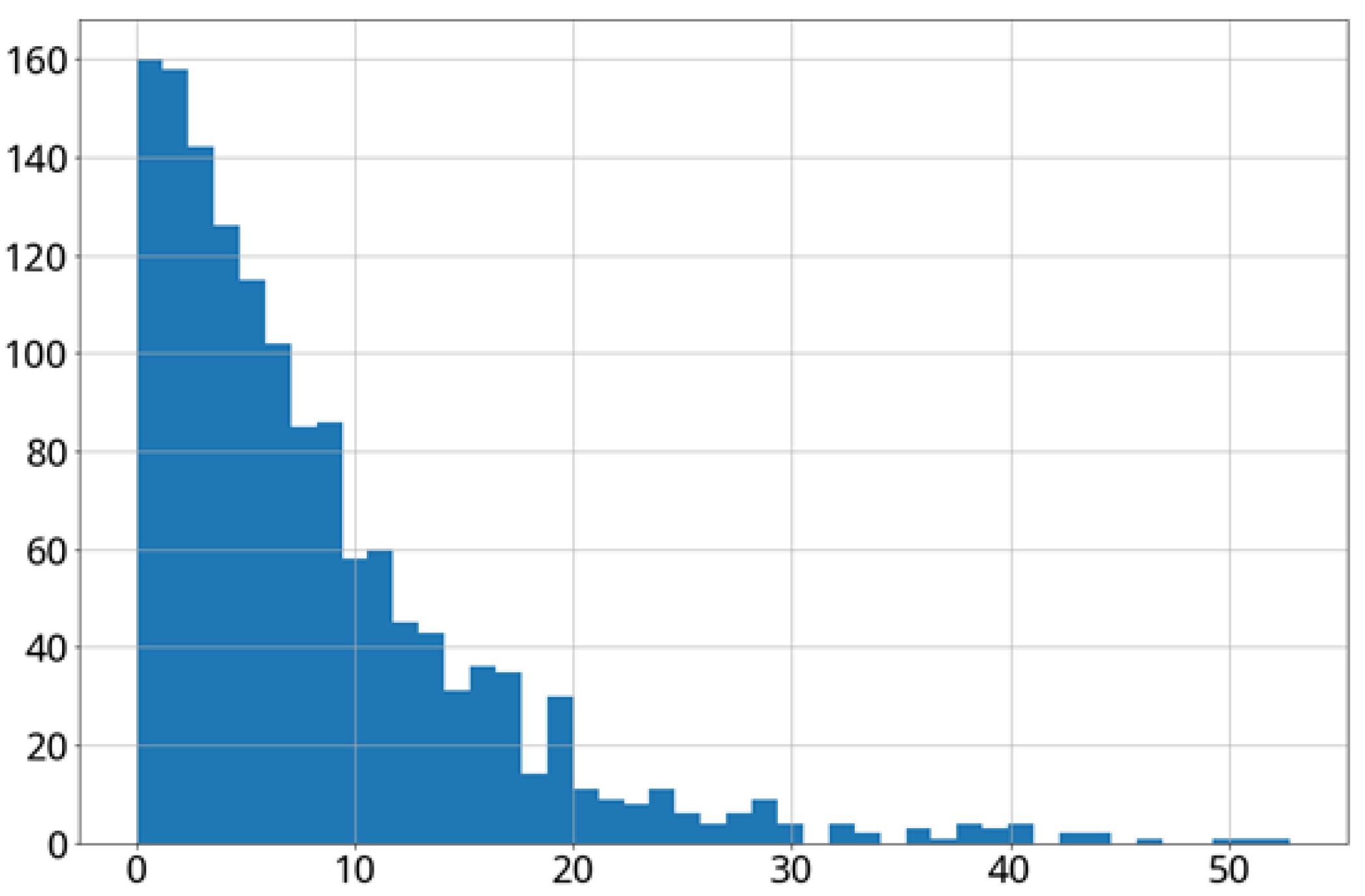
The multitemporal multispectral images that contain the ground-truth data were captured by miniature satellites operated by Planet Labs. For cabbages, the days to maturity are about 70 days, but this could vary according to seasons or regions. Therefore, this study gathered the data on 0–70 days of cabbage growth for the analysis, and it collected the satellite imagery data on the basis of the cadastre during the complete cabbage growth stages, according to the ground-truth data and the professional interpretations (
Figure 12,
Figure 13,
Figure 14 and
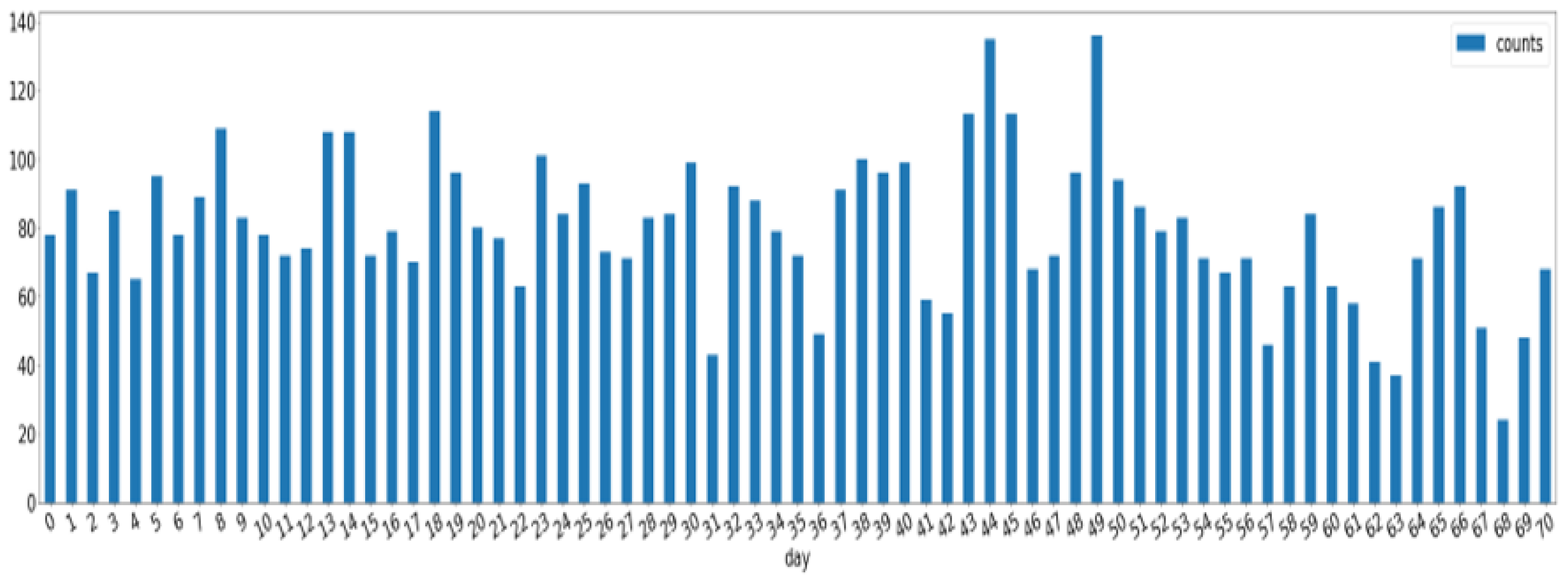
Figure 15). The data collection was conducted from 15 October 2018 to 19 March 2019, and 5654 records were collected for 0–70 days of the cabbage growth (
Figure 16).
3.2. Feature Selection
3.2.1. Spectral Feature Selection
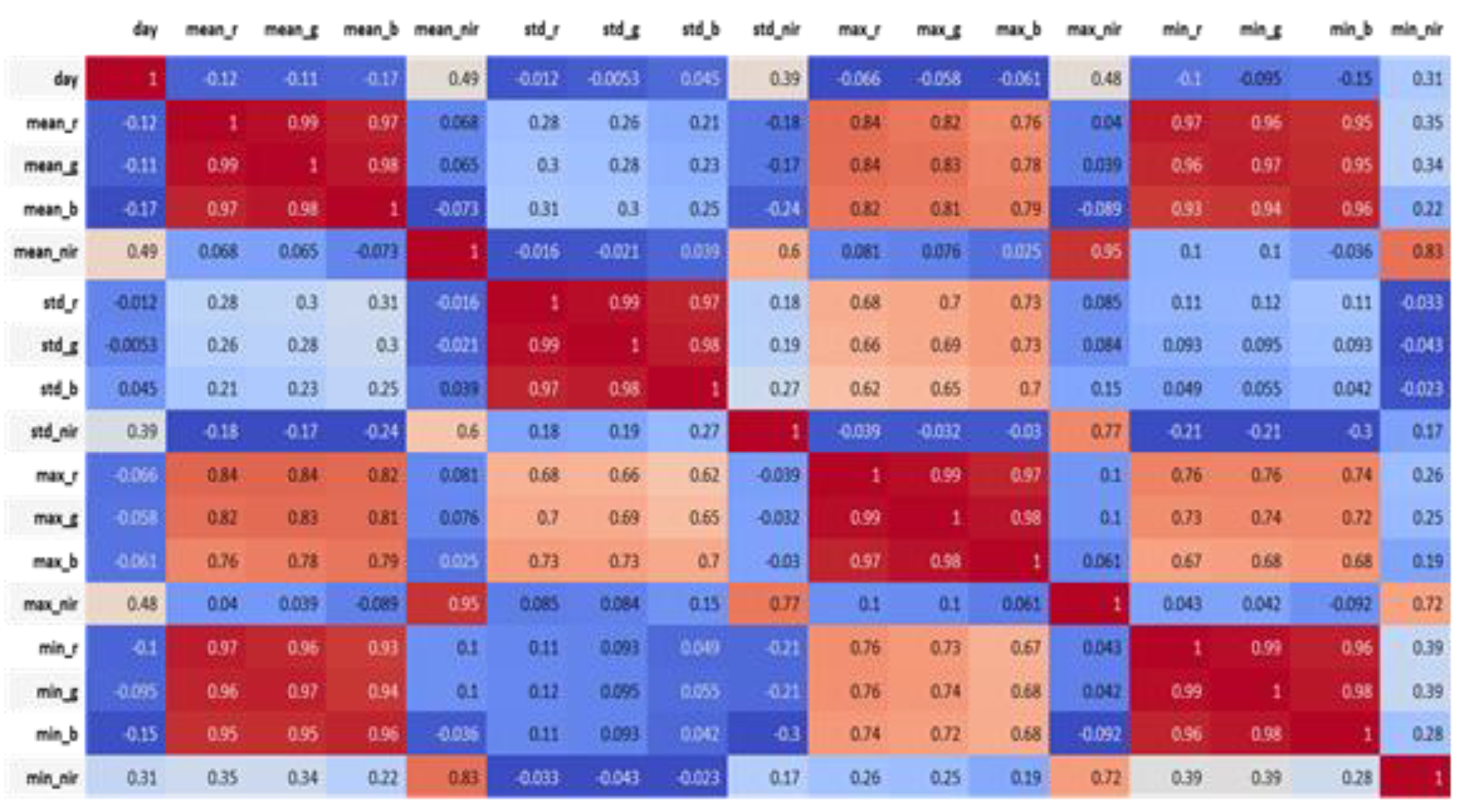
The multispectral satellite images that are used in this study are 3 m × 3 m pixels, and each pixel can reflect all of the visible RGB lights and the invisible infrared radiation (four spectral values in total). The corresponding pixel values are obtained according to the cadastral data. Next, a data analysis is conducted in order to distinguish the correlation between 16 attributes, including the mean, the std, the max and min of all the pixel values on each cadastre, and the days of cabbage growth (
Figure 17). The timeframe of 20 to 60 days of cabbage growth was selected to present the values of the spectral features, including the mean, max, and min of the infrared radiation (
Table 1).
3.2.2. Vegetation Index Feature Selection
The pixel spectral values were used to calculate eight types of vegetation indices, including the NDVI [
11,
12,
13], the infrared percentage vegetation index (IPVI) [
14], the cropping management factor index (CMFI), the band ratio (BR), the square band ratio (SQBR), the vegetable index (VI), the average brightness index (ABI), and the modified soil adjusted vegetation index (MSAVI) [
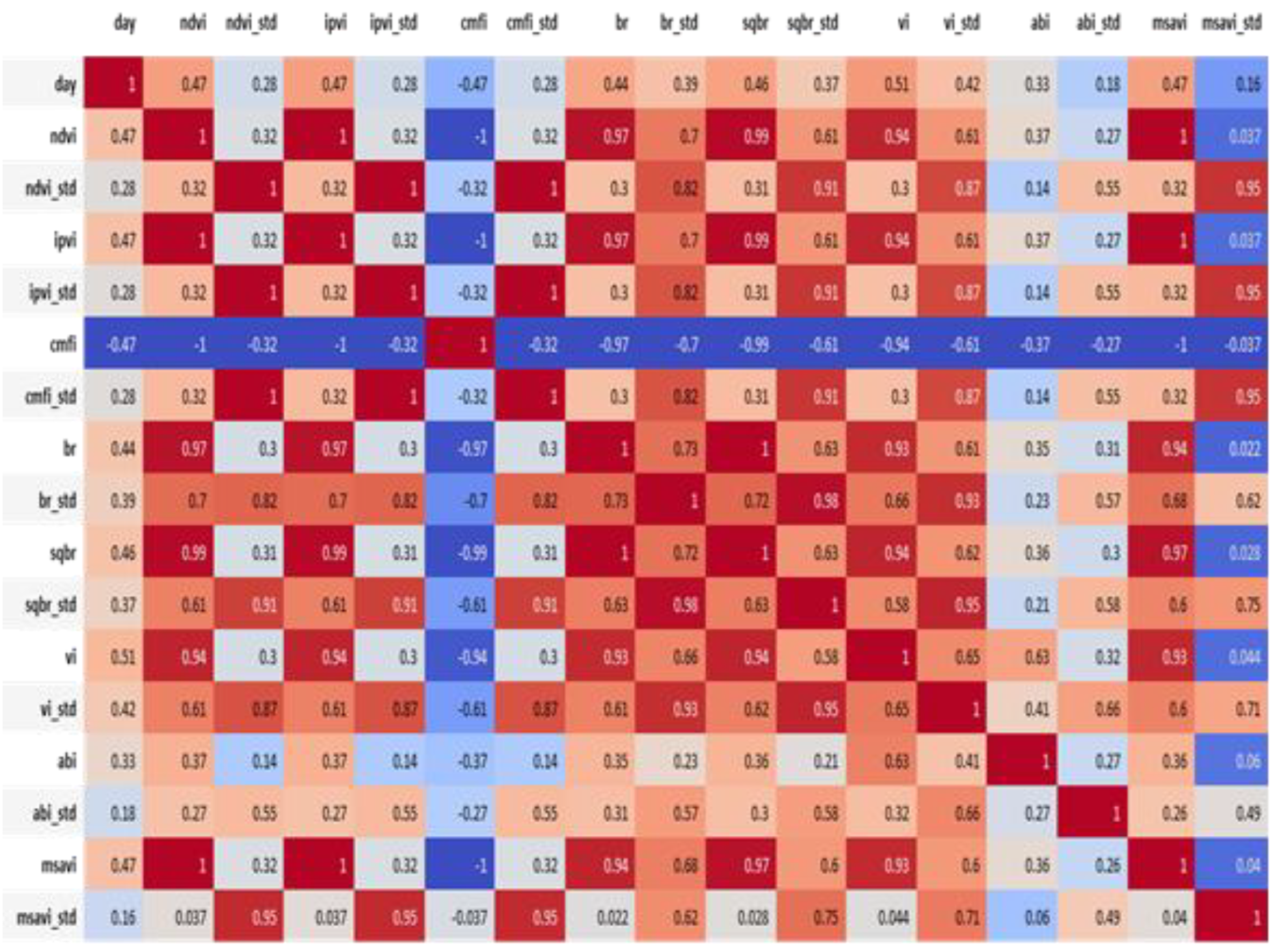
15,
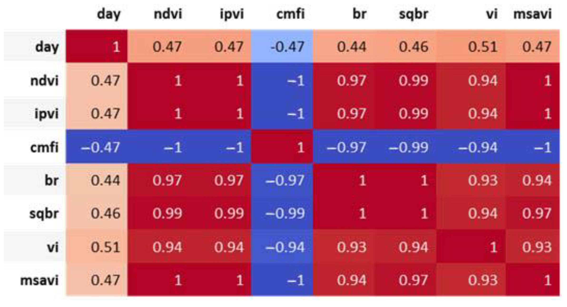
16]. A total of 16 attributes, including the mean and standard deviation of the individual vegetation index, were employed for the correlation analysis between the indices and the cabbage growth stages (i.e., the days of growth of the cabbages). The results are shown in
Figure 18 and
Figure 19. The period between 20 and 60 days indicates a highly positive correlation with the vegetation indices. In particular,
Figure 19 shows that the vegetation indices are more correlated, in comparison with the spectrum information, to the days of growth of the cabbages. However, most of the vegetation indices are calculated on the basis of near-infrared and red-light values, which happen to be highly correlated. Therefore, only one of the three completely correlated (i.e., correlation coefficients equal to 1 or −1) vegetation indices, such as the NDVI (IPVI, MSAVI, CMFI), the BR (SQBR), or the VI, was adopted (as shown in
Table 2).
3.2.3. Texture Feature Selection
The texture features of the satellite images that are taken into account include: a total of 6 image gradient [
17] attributes (the mean and standard deviations of gx, gy, and gxy), and 13 attributes that are derived from the GLCM method, which makes a total of 19 attributes. However, the correlation analysis shows that all of the texture features are not correlated with the days of growth of the cabbages (
Table 3). The reason may be that the resolution of the satellite imagery that was used was not high enough. Therefore, these features were not included in the model training.
3.2.4. Threshold Feature Selection
In order to increase the model prediction accuracy, the respective thresholds for the abovementioned features that were strongly correlated to the cabbage growth stages (namely, the near-infrared spectrum value and the NDVI, the BR, and the VI, which are the three vegetation indices) were used to filter the noise. The range of each of these features was defined by their induvial maximum and minimum values. For each of the four features, the 5654 samples were partitioned into three subsets according to their range values (see
Table 4). Two threshold candidates were obtained for each feature. For example, one of the thresholds (2588) for the NIR can be obtained by (5785−-990)/3 + 990. GBDT was applied five times in order to train the model on the basis of the cross-validation method, and the minimum mean square error (MSE) was adopted to select the optimal threshold values (
Table 5).
Once the optimal threshold value for each of the four features was determined, the additional 20 features for each image sample were defined as follows: the proportion of pixels with values above the threshold, and the mean/standard deviations of pixels with values above/below the threshold. The features are listed in
Appendix A.
3.2.5. Features Defined by the Differences between Two Consecutive Satellite Images
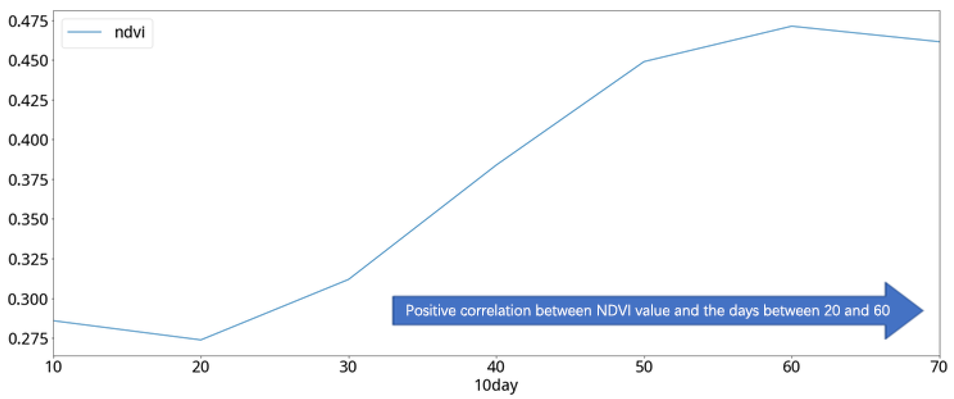
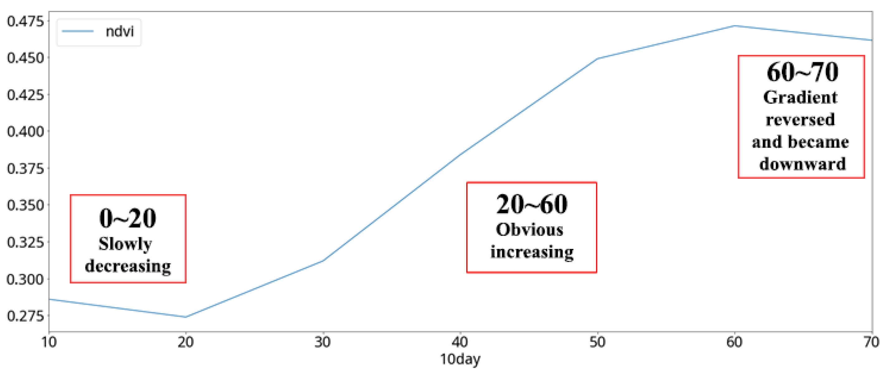
In the analysis of the cabbage vegetative index, the NDVI curve of the cabbage in different periods, which is averaged in units of 10 days, shows a significant positive correlation between the 20th and 60th days of the cabbage-growing period (
Figure 20). Compared to the growth stages of cabbage (
Table 6), the NDVI values of the cabbage show a rising trend in both the mature stage and the cupping stage (
Figure 21). Considering the result from the previous comparison, it can be inferred that the NDVI growth rate of the two consecutive satellite images can be used to effectively predict the growth stage of cabbages. Therefore, the individual difference values of the two consecutive images of each of the previously mentioned features were selected as the features to be used in this study, as shown in
Table 7.
3.2.6. Feature Summary
In summary, this study uses a total of 54 image features, 3 near-infrared light features (the average, standard deviation, and maximum values), 3 vegetation index features (NDVI, BR, and VI), 20 features that were obtained from near-infrared light, the NDVI, the BR, and the VI after threshold filtering (proportion of pixels with values above the threshold, and mean/standard deviation values of pixels with values above/below the threshold), and 1 feature that indicates the day of the year that the image was captured. So far, there are 27 features listed above, and the individual difference value for each feature was calculated on the basis of two consecutive images, which adds up to 54 features for the data mining (see
Appendix A).
3.3. Modeling and Verification
The collected ground-truth data, along with the location information, consist of a total of 735 samples, among which 220 samples were randomly selected for testing, and the remaining 515 samples were used for the cross-validation training of the regression and classification models.
3.3.1. GBDT Regression Analysis
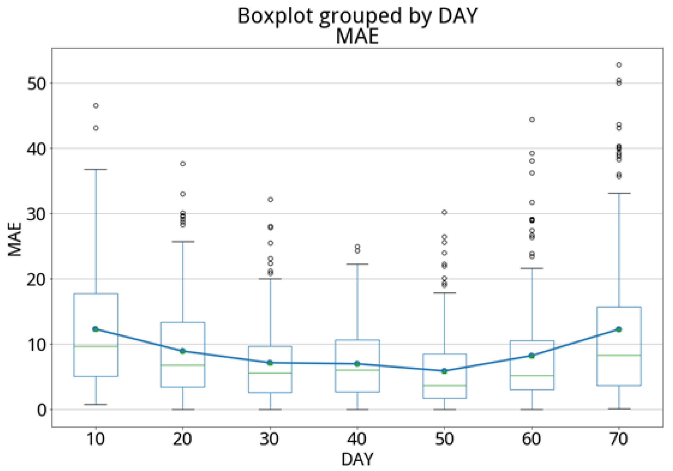
The GBDT regression technique was applied to the testing set (with 220 samples) to predict the growth stage of the cabbage from Day 0 to Day 70. The experimental results are shown in
Table 8 and
Figure 22. The average error is 8.17 days, with 75% of the prediction errors within 11 days, which are summarized in
Table 9 and
Figure 22.
3.3.2. GBDT Classification Analysis
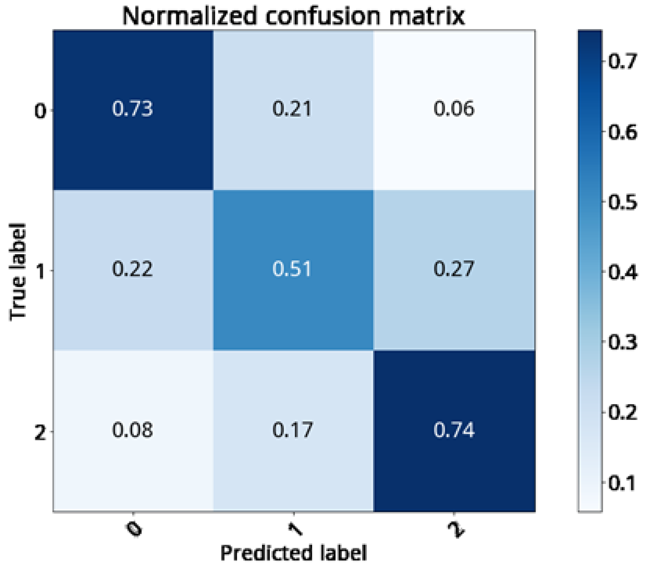
The GBDT classification technique was applied to the testing set (with 220 samples) to identify the growth status of the cabbage from three different stages: namely, the cupping, early heading, and mature stages. The experimental results are shown in
Table 10 And
Figure 23 and the confusion matrix shown in
Figure 24. The classification recalls are 73, 51 and 74%, respectively. If the growth status of cabbage has been divided into two stages instead of three (namely, within 40 days and beyond 40 days), then the prediction recalls become 83 and 76%, respectively. The results are shown in
Table 11 and
Figure 25.
3.4. Programing Language and Libraries
This study uses Python, which is the most popular language for data analysis, data science, and machine learning. The biggest advantage of using Python is that there are plenty of libraries to support the latest technologies.
Table 12 lists all the libraries or packages that were used to conduct the experiments.
4. Discussion
This paper first attempts to use multiperiod multispectral satellite image information for training a deep learning model. Cabbage is an important short-term cash crop, which often encounters an imbalance between production and sales. This study uses GBDT for the regression analysis. With the limited amount of training data (i.e., 735 ground-truth images), the trained model was able to automatically predict the days of growth of the cabbage on the basis of the satellite images of the cabbage field, with an average error of 8.17 days, and 75% of the predictions having errors less than 11 days. (Note: the cabbage’s growth cycle is between 0 and 70 days.) Moreover, this study also uses GBDT for the classification analysis. First, if the cabbage growth status is divided into three stages (the cupping, early heading, and mature stages), then the prediction recalls for these three stages are 73, 51, and 74%, respectively. Second, if the growth status is divided into two stages (within 40 days and beyond 40 days), then the prediction recalls become 83 and 76%, respectively. These results show that, with the appropriate data mining technology, multiperiod and multispectral satellite image information can be used to automatically determine the days of growth and the growth stages of cabbage. If the government’s agriculture department could make use of such results, by knowing the harvested area of cabbage, government staffs can prepare and respond early when the possibility of an imbalance between production and sales emerges.
In addition, the field survey APP that was developed in this study for collecting the ground-truth data, together with the cadastral information, have proven to come in handy. The ground-truth data for the experiments were captured with the help from colleagues at the Yunlin Irrigation Association. The collected photos were manually examined before use as training data. The mobile devices were also screened to ensure that the data obtained by their GPS and digital compass sensors, as well as the alignment information set by the APP, were accurate. The cadastral information of the image can be calculated by these data, which provide the ground-truth information for the AI training of the aerial and satellite images. The experimental result is an important opportunity for agricultural production surveys. If this APP can be adopted by agricultural administration offices, the on-site surveys of agricultural products can be more accurate. Previously, only statistical data from townships were available, but, with the help of this APP, it is possible to obtain the cadastral information. When there is an important crop that needs production guidance, the producer can be found through the cadastral information so that the related actions can be directly and effectively performed, or, in cases where the agricultural product is damaged because of natural disasters, farmers can use the APP to take pictures and to apply for assistance so that the rescue can take place more efficiently. Moreover, this APP is easy to use, which makes it a handy tool for agricultural market reporters during agricultural investigations. It can also be used by general users in order to collect updated agricultural information through mass outsourcing, which has the advantages of saving time, manpower, and costs.
5. Conclusions
The results of the proposed method have verified that data mining technology can be used to predict the growth stages or days of growth of cabbage by analyzing the multispectral satellite images. For future works, besides the further improvement of the model, it is also necessary to develop a recognition method to identify cabbage fields by multispectral satellite images. The combination of these two methods would become a highly effective solution for assisting the production and sales of cabbage.
Future research could use the Assisted Global Positioning System, which is a technology that uses cell-phone-based station signals to obtain GPS locations more accurately and quickly, and to find the location of photographed objects. In addition, it may be possible to try other crops for growth prediction, and, possibly, the methods of this study could be applied to other similar species for growth prediction.
Author Contributions
D.-C.H.: conceptualization, methodology, data curation, validation, formal analysis, visualization, writing—original draft; F.H.: formal analysis, visualization, writing—original draft; F.J.T.: software, validation, writing—original draft; T.-Y.W.: conceptualization, methodology, project administration; Y.-C.L.: investigation. All authors have read and agreed to the published version of the manuscript.
Funding
This work was funded by the Ministry of Science and Technology, Taiwan under Grant No MOST 110-2221-E-020-023, and MOST 108-2321-B-197-004.
Institutional Review Board Statement
Not applicable.
Informed Consent Statement
Not applicable.
Data Availability Statement
Not applicable.
Acknowledgments
This study was supported by the Ministry of Science and Technology, Taiwan, under grant No. MOST 110-2221-E-020-023, and MOST 108-2321-B-197-004.
Conflicts of Interest
The authors declare no conflict of interest.
Appendix A
| No. | Category | Features | Attributes | Description | If Used? |
|---|
| 1 | Date | Month | month | Captured month | |
| 2 | Day | date | Captured day | |
| 3 | Day of the year | yday | The day of the year that the image was captured. | Y |
| 8 | Spectrum | Red-light average | mean_r | | |
| 9 | Red-light standard deviation | std_r | | |
| 10 | Red-light max value | max_r | | |
| 11 | Red-light min value | min_r | | |
| 12 | Green-light average | mean_g | | |
| 13 | Green-light standard deviation | std_g | | |
| 14 | Green-light max value | max_g | | |
| 15 | Green-light min value | min_g | | |
| 16 | Blue-light average | mean_b | | |
| 17 | Blue-light standard deviation | std_b | | |
| 18 | Blue-light max value | max_b | | |
| 19 | Blue-light min value | min_b | | |
| 20 | Near-infrared-light average | mean_nir | | Y |
| 21 | Near-infrared-light standard deviation | std_nir | | Y |
| 22 | Near-infrared-light max value | max_nir | | Y |
| 23 | Near-infrared-light min value | min_nir | | |
| 24 | Texture | Image x gradient average | gx_mean | RGB image x gradient | |
| 25 | Image x gradient standard deviation | gx_std | RGB image x gradient | |
| 26 | Image y gradient average | gy_mean | RGB image y gradient | |
| 27 | Image y gradient standard deviation | gy_std | RGB image y gradient | |
| 28 | Image x and y gradients average | gxy_mean | RGB image x and y gradients | |
| 29 | Image x and y gradients standard deviation | gxy_std | RGB image x and y gradients | |
| 30 | Haralick texture | haralick_1 | GLCM gives 13 features | |
| 31 | haralick_2 | |
| 32 | haralick_3 | |
| 33 | haralick_4 | |
| 34 | haralick_5 | |
| 35 | haralick_6 | |
| 36 | haralick_7 | |
| 37 | haralick_8 | |
| 38 | haralick_9 | |
| 39 | haralick_10 | |
| 40 | haralick_11 | |
| 41 | haralick_12 | |
| 42 | haralick_13 | |
| 43 | Vegetation Index | Normalized difference vegetation index | ndvi | Average | Y |
| 44 | ndvi_std | Standard deviation | |
| 45 | Infrared percentage vegetation index | ipvi | Average | |
| 46 | ipvi_std | Standard deviation | |
| 47 | Cropping management factor index | cmfi | Average | |
| 48 | cmfi_std | Standard deviation | |
| 49 | Band ratio | br | Average | Y |
| 50 | br_std | Standard deviation | |
| 51 | Square band ratio | sqbr | Average | |
| 52 | sqbr_std | Standard deviation | |
| 53 | Vegetation index | vi | Average | Y |
| 54 | vi_std | Standard deviation | |
| 55 | Average brightness index | abi | Average | |
| 56 | abi_std | Standard deviation | |
| 57 | Modified soil adjusted vegetation index | msavi | Average | |
| 58 | msavi_std | Standard deviation | |
| 59 | Threshold | Proportion of pixels with values above the near-infrared threshold | nir_ratio | Threshold 4186 | Y |
| 60 | The mean value of pixels with values above the near-infrared threshold | nir_mean | Y |
| 61 | The standard deviation value of pixels with values above the near-infrared threshold | nir_std | Y |
| 62 | The mean value of pixels with values below the near-infrared threshold | nir_un_mean | Y |
| 63 | The standard deviation value of pixels with values below the near-infrared threshold | nir_un_std | Y |
| 64 | Proportion of pixels with values above the NDVI threshold | ndvi_ratio | Threshold 0.47 | Y |
| 65 | The mean value of pixels with values above the NDVI threshold | ndvi_mean | Y |
| 66 | The standard deviation value of pixels with values above the NDVI threshold | ndvi_std | Y |
| 67 | The mean value of pixels with values below the NDVI threshold | ndvi_un_mean | Y |
| 68 | The standard deviation value of pixels with values below the NDVI threshold | ndvi_un_std | Y |
| 69 | Proportion of pixels with values above the BR threshold | vi_ratio | Threshold 3.02 | Y |
| 70 | The mean value of pixels with values above the BR threshold | vi_mean | Y |
| 71 | The standard deviation value of pixels with values above the BR threshold | vi_std | Y |
| 72 | The mean value of pixels with values below the BR threshold | vi_un_mean | Y |
| 73 | The standard deviation value of pixels with values below the BR threshold | vi_un_std | Y |
| 74 | Proportion of pixels with values above the VI threshold | abi_ratio | Threshold 1034 | Y |
| 75 | The mean value of pixels with values above the VI threshold | abi_mean | Y |
| 76 | The standard deviation value of pixels with values above the VI threshold | abi_std | Y |
| 77 | The mean value of pixels with values below the VI threshold | abi_un_mean | Y |
| 78 | The standard deviation value of pixels with values below the VI threshold | abi_un_std | Y |
| 79 | Difference | The difference values of all the features used. | *_diff | Only calculate features that are marked Y in the last column. | |
References
- Pluto-Kossakowska, J. Review on Multitemporal Classification Methods of Satellite Images for Crop and Arable Land Recognition. Agriculture 2021, 11, 999. [Google Scholar] [CrossRef]
- Fernández-Sellers, M.; Siesto, G.; Lozano-Tello, A.; Clemente, P.J. Finding a suitable sensing time period for crop identification using heuristic techniques with multi-temporal satellite images. Int. J. Remote Sens. 2021, 1–18. [Google Scholar] [CrossRef]
- Felegari, S.; Sharifi, A.; Moravej, K.; Amin, M.; Golchin, A.; Muzirafuti, A.; Tariq, A.; Zhao, N. Integration of Sentinel 1 and Sentinel 2 Satellite Images for Crop Mapping. Appl. Sci. 2021, 11, 10104. [Google Scholar] [CrossRef]
- Haralick, R.M.; Shanmugam, K.; Dinstein, I.H. Textural features for image classification. IEEE Trans. Syst. Man Cybern. 1973, 610–621. [Google Scholar] [CrossRef] [Green Version]
- Miyamoto, E.; Merryman, T. Fast Calculation of Haralick Texture Features; Human Computer Interaction Institute, Carnegie Mellon University: Pittsburgh, PA, USA, 2005. [Google Scholar]
- Nussbaum, S.; Niemeyer, I.; Canty, M. SEATH-a new tool for automated feature extraction in the context of object-based image analysis. In Proceedings of the 1st International Conference on Object-Based Image Analysis (OBIA), Salzburg, Austria, 4–5 July 2006. [Google Scholar]
- Wan, S.; Chang, S.-H.; Peng, C.-T.; Chen, Y.-K. A novel study of artificial bee colony with clustering technique on paddy rice image classification. Arab. J. Geosci. 2017, 10, 1–13. [Google Scholar] [CrossRef]
- Wolter, P.T.; Mladenoff, D.J.; Host, G.E.; Crow, T.R. Using multi-temporal landsat imagery. Photogramm. Eng. Remote Sens. 1995, 61, 1129–1143. [Google Scholar]
- Vens, C.; Struyf, J.; Schietgat, L.; Džeroski, S.; Blockeel, H. Decision trees for hierarchical multi-label classification. Mach. Learn. 2008, 73, 185–214. [Google Scholar] [CrossRef] [Green Version]
- Bentéjac, C.; Csörgő, A.; Martínez-Muñoz, G. A comparative analysis of gradient boosting algorithms. Artif. Intell. Rev. 2021, 54, 1937–1967. [Google Scholar] [CrossRef]
- Burgan, R.E. Monitoring Vegetation Greenness with Satellite Data; US Department of Agriculture, Forest Service, Intermountain Research Station: Ogden, UT, USA, 1993; Volume 297.
- Elvidge, C.D.; Chen, Z. Comparison of broad-band and narrow-band red and near-infrared vegetation indices. Remote Sens. Environ. 1995, 54, 38–48. [Google Scholar] [CrossRef]
- Rouse, J.W., Jr.; Haas, R.H.; Schell, J.; Deering, D. Monitoring the Vernal Advancement and Retrogradation (Green Wave Effect) of Natural Vegetation; NASA: Washington, DC, USA, 1973.
- Crippen, R.E. Calculating the vegetation index faster. Remote Sens. Environ. 1990, 34, 71–73. [Google Scholar] [CrossRef]
- Huete, A.R. A soil-adjusted vegetation index (SAVI). Remote Sens. Environ. 1988, 25, 295–309. [Google Scholar] [CrossRef]
- Qi, J.; Chehbouni, A.; Huete, A.R.; Kerr, Y.H.; Sorooshian, S. A modified soil adjusted vegetation index. Remote Sens. Environ. 1994, 48, 119–126. [Google Scholar] [CrossRef]
- Jacobs, D. Image Gradients. Available online: https://www.cs.umd.edu/~djacobs/CMSC426/ImageGradients.pdf (accessed on 10 December 2021).
Figure 1.
Multitemporal satellite image analysis.
Figure 1.
Multitemporal satellite image analysis.
Figure 2.
Data mining procedure.
Figure 2.
Data mining procedure.
Figure 3.
The crucial technique for the agricultural survey APP is to measure the distance between the camera and the object.
Figure 3.
The crucial technique for the agricultural survey APP is to measure the distance between the camera and the object.
Figure 4.
While taking photos, the proposed agricultural survey APP offers a reference point on the target object, and it has a GPS variation detection function.
Figure 4.
While taking photos, the proposed agricultural survey APP offers a reference point on the target object, and it has a GPS variation detection function.
Figure 5.
Vector diagram of the CCD center and the target object when photographing.
Figure 5.
Vector diagram of the CCD center and the target object when photographing.
Figure 6.
Differential image classification flowchart.
Figure 6.
Differential image classification flowchart.
Figure 7.
K-fold model cross validation.
Figure 7.
K-fold model cross validation.
Figure 8.
Time series cross validation.
Figure 8.
Time series cross validation.
Figure 9.
Flowchart of the methodology.
Figure 9.
Flowchart of the methodology.
Figure 10.
Backstage interpretations of the field survey images by an agricultural professional.
Figure 10.
Backstage interpretations of the field survey images by an agricultural professional.
Figure 11.
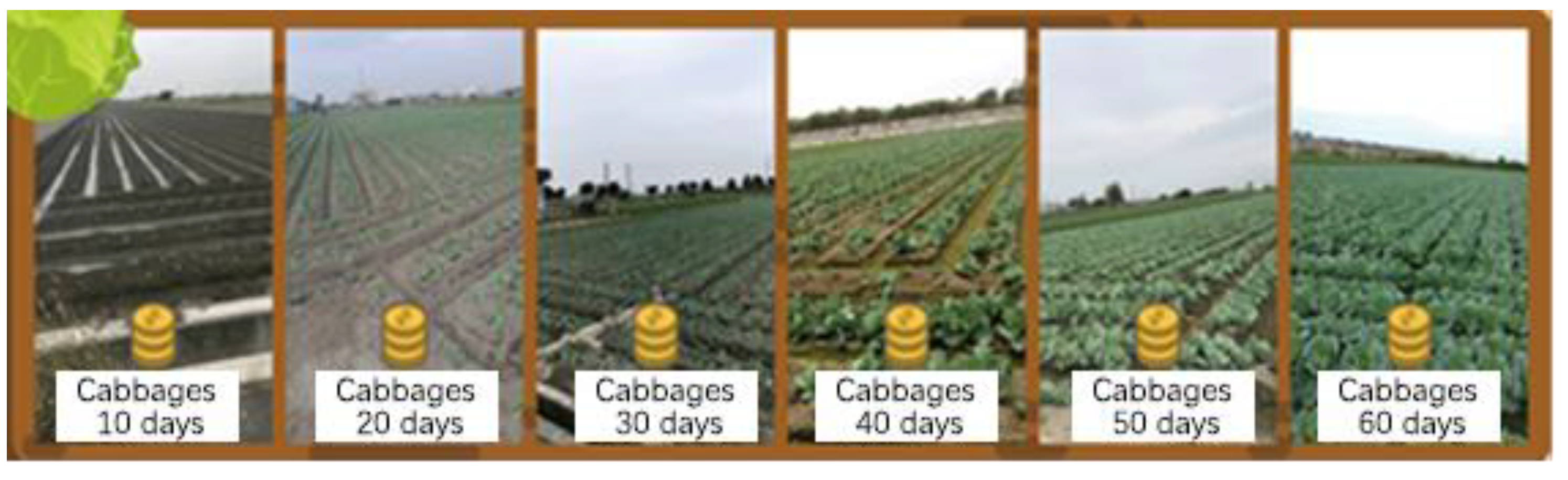
Agricultural professionals interpret the growth days of cabbages according to the field survey images.
Figure 11.
Agricultural professionals interpret the growth days of cabbages according to the field survey images.
Figure 12.
Satellite images of cabbages (10 days).
Figure 12.
Satellite images of cabbages (10 days).
Figure 13.
Satellite images of cabbages (30 days).
Figure 13.
Satellite images of cabbages (30 days).
Figure 14.
Satellite images of cabbages (60 days).
Figure 14.
Satellite images of cabbages (60 days).
Figure 15.
Multitemporal satellite images of cabbages under the same parcel number.
Figure 15.
Multitemporal satellite images of cabbages under the same parcel number.
Figure 16.
Number of satellite images on days of cabbage growth.
Figure 16.
Number of satellite images on days of cabbage growth.
Figure 17.
Correlation between spectral features and cabbage growth stages.
Figure 17.
Correlation between spectral features and cabbage growth stages.
Figure 18.
Correlations between vegetation index features and cabbage growth stages.
Figure 18.
Correlations between vegetation index features and cabbage growth stages.
Figure 19.
High or even complete correlations between pairs of vegetation index features.
Figure 19.
High or even complete correlations between pairs of vegetation index features.
Figure 20.
Correlation analysis between cabbage growth stages and NDVI values.
Figure 20.
Correlation analysis between cabbage growth stages and NDVI values.
Figure 21.
Cabbage growth stages vs. NDVI values.
Figure 21.
Cabbage growth stages vs. NDVI values.
Figure 22.
Growth stage prediction results of cabbage from Day 0 to Day 70.
Figure 22.
Growth stage prediction results of cabbage from Day 0 to Day 70.
Figure 23.
Distribution chart of the growth stage prediction of cabbage.
Figure 23.
Distribution chart of the growth stage prediction of cabbage.
Figure 24.
Confusion matrix of the cabbage growth stage classification from cupping, early heading, and mature stages.
Figure 24.
Confusion matrix of the cabbage growth stage classification from cupping, early heading, and mature stages.
Figure 25.
The confusion matrix of the cabbage growth stage classification from early growth and mid-heading stages.
Figure 25.
The confusion matrix of the cabbage growth stage classification from early growth and mid-heading stages.
Table 1.
Correlation coefficients between spectral features and cabbage growth stages.
Table 1.
Correlation coefficients between spectral features and cabbage growth stages.
| Spectral Features | Correlation Coefficient |
|---|
| mean_nir Mean value of NIR | 0.486128 |
| std_nir Standard deviation of NIR | 0.393943 |
| max_nir Maximum of NIR | 0.478906 |
Table 2.
Correlation analysis between vegetation indices and cabbage growth stages.
Table 2.
Correlation analysis between vegetation indices and cabbage growth stages.
| Vegetation Index | Correlation Coefficients |
|---|
| NDVI | 0.47121 |
| IPVI | 0.47121 |
| CMFI | −0.47121 |
| BR | 0.443567 |
| SQBR | 0.458123 |
| VI | 0.508448 |
| MSAVI | 0.468535 |
Table 3.
Correlations between texture features and cabbage growth stages.
Table 3.
Correlations between texture features and cabbage growth stages.
| Texture Feature | Correlation Coefficients |
|---|
| haralick_1 | −0.012057 |
| haralick_2 | −0.011231 |
| haralick_3 | 0.004898 |
| haralick_4 | −0.029392 |
| haralick_5 | 0.065032 |
| haralick_6 | −0.123112 |
| haralick_7 | −0.029654 |
| haralick_8 | −0.054594 |
| haralick_9 | −0.016616 |
| haralick_10 | 0.016184 |
| haralick_11 | −0.009838 |
| haralick_12 | 0.060944 |
| haralick_13 | −0.014681 |
| gxy_mean | −0.004639 |
| gxy_std | 0.022363 |
| gx_mean | −0.002482 |
| gx_std | 0.005792 |
| gy_mean | 0.000629 |
| gy_std | 0.045106 |
Table 4.
Important features and their threshold candidates.
Table 4.
Important features and their threshold candidates.
| Features | Minimum | Maximum | Threshold Candidates
(3 Partitions) |
|---|
| NIR | 990 | 5785 | 2588, 4186 |
| NDVI | −0.09 | 0.76 | 0.19, 0.47 |
| BR | 0.83 | 7.4 | 3.02, 5.21 |
| VI | −519 | 4142 | 1034, 2588 |
Table 5.
The optimal threshold values for each feature on the basis of cross-validation method.
Table 5.
The optimal threshold values for each feature on the basis of cross-validation method.
| Features | Minimum | Maximum | Optimal Threshold Value |
|---|
| NIR | 990 | 5785 | 4186 |
| NDVI | −0.09 | 0.76 | 0.47 |
| BR | 0.83 | 7.4 | 3.02 |
| VI | −519 | 4142 | 1034 |
Table 6.
Cabbage growth stages.
Table 6.
Cabbage growth stages.
| Cabbage Growth Stages | Days |
|---|
| Cupping Stage | 0–40 |
| Early Heading Stage | 40, 50, 60 |
| Mature Stage | 70–80 |
Table 7.
Differences in individual features between two consecutive satellite images captured at the same location.
Table 7.
Differences in individual features between two consecutive satellite images captured at the same location.
| Day | ndvi | std_nir | … | std_nir_diff |
|---|
| 7 | 0.721168 | 647.696193 | … | NaN |
| 28 | 0.281660 | 1019.547319 | … | 371.851125 |
| 37 | 0.270601 | 1351.375908 | … | 331.828589 |
| 48 | 0.447606 | 1576.486765 | … | 225.110857 |
| 55 | 0.454097 | 1657.495210 | … | 81.008445 |
| 63 | 0.515093 | 1578.958585 | … | −78.536626 |
Table 8.
Growth stage prediction results of cabbage from Day 0 to Day 70.
Table 8.
Growth stage prediction results of cabbage from Day 0 to Day 70.
| Day | Count | Mean | Std. | Min. | 25% | 50% | 75% | Max. |
|---|
| 10 | 3.00 | 3.27 | 2.52 | 0.85 | 1.96 | 3.08 | 4.48 | 5.88 |
| 20 | 161.00 | 7.26 | 9.46 | 0.02 | 2.13 | 4.59 | 8.30 | 52.81 |
| 30 | 322.00 | 9.12 | 8.18 | 0.08 | 3.75 | 7.04 | 11.96 | 43.66 |
| 40 | 296.00 | 9.04 | 7.64 | 0.02 | 3.18 | 6.84 | 13.20 | 38.71 |
| 50 | 366.00 | 8.19 | 7.69 | 0.02 | 2.21 | 5.69 | 12.11 | 43.20 |
| 60 | 184.00 | 7.74 | 6.46 | 0.02 | 3.17 | 6.57 | 10.77 | 46.61 |
| 70 | 91.00 | 4.52 | 3.49 | 0.19 | 1.78 | 3.57 | 7.20 | 13.64 |
Table 9.
Cabbage growth stage prediction summary.
Table 9.
Cabbage growth stage prediction summary.
| Statistics | MAE |
|---|
| Count | 1423 |
| Mean | 8.17072 |
| Std. | 7.746078 |
| Min. | 0.017453 |
| 25% | 2.672483 |
| 50% | 5.971289 |
| 75% | 11.03056 |
| Max. | 52.809956 |
Table 10.
Growth status classification results of cabbage from cupping, early heading, and mature stages.
Table 10.
Growth status classification results of cabbage from cupping, early heading, and mature stages.
| Stages | Precision | Recall | F1-Score | Support |
|---|
Cupping Stage
(0–25 days) | 0.69 | 0.73 | 0.71 | 415 |
Early Heading Stage
(25–40 days) | 0.50 | 0.51 | 0.50 | 379 |
Mature Stage
(40–70 days) | 0.79 | 0.74 | 0.77 | 629 |
| Avg./Total | 0.68 | 0.68 | 0.68 | 1423 |
Table 11.
Growth stage classification results of cabbage from early growth and mid-heading stages.
Table 11.
Growth stage classification results of cabbage from early growth and mid-heading stages.
| Stages | Precision | Recall | F1-Score | Support |
|---|
Early Growth Stage
(0~40 days) | 0.81 | 0.83 | 0.82 | 794 |
Mid-Heading Stage
(40~70 days) | 0.78 | 0.76 | 0.77 | 629 |
| Avg./Total | 0.80 | 0.80 | 0.80 | 1423 |
Table 12.
Python libraries or packages used in this study.
Table 12.
Python libraries or packages used in this study.
| Functionality | Libraries or Packages |
|---|
| Data Manipulation | Pandas |
| Image Preocessing | cv2 |
| Reading Satellite Images | Tifffile |
| Model Training | scikit-learn |
| Model | LightGBM |
| Publisher’s Note: MDPI stays neutral with regard to jurisdictional claims in published maps and institutional affiliations. |
© 2022 by the authors. Licensee MDPI, Basel, Switzerland. This article is an open access article distributed under the terms and conditions of the Creative Commons Attribution (CC BY) license (https://creativecommons.org/licenses/by/4.0/).


