Assessing the Efficiency of Remote Sensing and Machine Learning Algorithms to Quantify Wheat Characteristics in the Nile Delta Region of Egypt

Abstract

Monitoring strategic agricultural crops in terms of crop growth performance, by accurate cost-effective and quick tools is crucially important in site-specific management to avoid crop reductions. The availability of commercial high resolution satellite images with high resolution (spatial and spectral) as well as in situ spectra measurements can help decision takers to have deep insight on crop stress in a certain region. The research attempts to examine remote sensing dataset for forecasting wheat crop (Sakha 61) characteristics including the leaf area index (LAI), plant height (plant-h), above ground biomass (AGB) and Soil Plant Analysis Development (SPAD) value of wheat across non-stress, drought and salinity-induced stress in the Nile Delta region. In this context, the ability of in situ spectroradiometry measurements and QuickBird high resolution images was evaluated in our research. The efficiency of Random Forest (RF) and Artificial Neural Network (ANN), mathematical models was assessed to estimate the four measured wheat characteristics based on vegetation spectral reflectance indices (V-SRIs) extracted from both approaches and their interactions. Field surveys were carried out to collect in situ spectroradiometry measurements concomitant with the acquisition of QuickBird imagery. The results demonstrated that several V-SRIs extracted from in situ spectroradiometry data and the QuickBird image correlated with the LAI, plant-h, AGB, and SPAD value of wheat crop across the study site. The determination coefficient (R²) values of the association between V-SRIs of in situ spectroradiometry data and various determined wheat characteristics varied from 0.26 to 0.85. The ANN-GSIs-3 was found to be the optimum predictive model, demonstrating a greater relationship between the advanced features and LAI. The three features of V-SRIs comprised in this model were strongly significant for the prediction of LAI. The attained results indicated high R² values of 0.94 and 0.86 for the training and validation phases. The ANN-GSIs-3 model constructed for the determination of chlorophyll in the plant which had higher performance expectations (R² = 0.96 and 0.92 for training and validation datasets, respectively). In conclusion, the results of our study revealed that high resolution remote sensing images such as QuickBird or similar imagery, and in situ spectroradiometry measurements have the feasibility of providing necessary crop monitoring data across non-stressed and stressed (drought and salinity) conditions when integrating V-SRIs with ANN and RF algorithms.

1. Introduction

The scarcity of freshwater resources is considered an essential consideration in both arid and semi-arid environments and thus the accessibility of water resources of low quality (e.g., drainage water, wastewater, and brackish water) has become a more important consideration in supplementing supply [1,2,3,4]. Broadly, irrigation efficiency within cultivated sectors in many regions worldwide is low and remarkable water savings could be accomplished via a more precise, robust and efficient management of available irrigation water resources. Jones [5] confirmed that water stress is the main factor influencing the limitations of crop production and therefore crop water requirements should be satisfied to avoid low crop productivity.

In the Nile Delta region, grain crop production is mainly hindered by issues of water availability and salinity as a result of limited water resources [6]. Detecting stress in agricultural crops across vast areas by traditional methods (e.g., point-sampling) is time consuming and costly and is sometimes unrepresentative in offering a spatial panorama of stress patterns [4,7,8,9]. Precise and fast assessment and monitoring ways for crop health status to quantify crop characteristics can enhance site-specific management to obtain a higher crop productivity in comparison to traditional monitoring techniques. In this regard, remote sensing of different platforms may offer a reliable tool in precision agriculture [10,11,12,13]. Drought and salinity stress are considered major inhibitors of strategic crop production (e.g., wheat, corn and rice), and more energies to spot their effects for irrigation management strategies are compulsory as several studies have quantitatively evaluated the potential of remote sensing to identify cultivated areas that are suffering from water and/or salinity stress [14]. Irrigation and water salinity management procedures must be carefully managed to maximize water use efficiency and to avoid higher salinity levels in the root zone by adding the optimum rates of water [6,15,16]. Observing crop health status is normally dependent upon destructive sampling, which as mentioned earlier is time consuming, costly, and is an unrepresentative process. A reliable alternative is the utilization of remote sensing of different platforms as a fast and robust tool that integrates the crop response to the negative effects of drought and salinity.

Expected climate change and global warming over the present century will lead to increase evaporation and as a result, a lack of freshwater resources linked to water stress, which is an obstacle to the world’s food security [17,18,19]. Basically, water stress and/or salinity stress of soil disrupt the main plant functions, resulting in significant decreases in several morphological and physiological crop features, such as chlorophyll concentration, the water status of plants, photosynthetic activity, stomatal conductance and aerial fresh biomass, causing significant losses in crop productivity [20,21,22,23]. In this context, the accurate and instantaneous detection of drought and salinity stress impact on both the local and regional scales is fundamentally important for achieving high crop yields and maximizing water productivity.

Remote sensing of different platforms has been used to monitor agricultural crops status over the past few decades. It is able to provide instantaneous information over vast cultivated regions of high economic importance, such as wheat and corn [6,24,25]. Such instantaneous information related to crop productivity is fundamentally crucial for experts and decision makers, from small-scale growers to the national authority, offering a step forward for maximizing crop yield whilst using available water resources in a more efficient way. Recently, the launch of a new generation of satellites (QuickBird, GeoEye 1, 2, and 3) with high capacities has been utilized in the precision farming field, which in reality would be useful in site-specific management. Many previous studies have revealed the feasibility of satellite images to quantify various crop characteristics (e.g., biochemical and biophysical). These include, for example, the identification of chlorophyll concentration [6,26,27,28]; the prediction of yield [29,30,31,32]; measuring leaf area index (LAI) [33,34,35]; the identification of nitrogen status [36]; estimating above-ground biomass [37]; quantifying evapotranspiration [38]; and the detection of crop disease [39,40]. These above-mentioned studies used satellite-based V-SRIs for the identification of crop characteristics, showing the robustness of high resolution satellite imagery (<2 m) to assess crop growth performance and to avoid stress on crops at a local scale. A decent number of satellite-based indices (Vegetation-SRIs) have been utilized as indicators of crop growth performance and yield. For instance, LAI and above ground biomass were noticed to be responsive to the Green Normalized Vegetation Index (GNDVI) and the simple ratio (SR) [41,42]. The sensitivity of the Red-edge Triangle Vegetation Index (RTVI) and other red-edge based indices to LAI and biomass has been demonstrated [41]. Intra-field variability can also be mapped using QuickBird at broad scales. Monitoring crop growth performance using ground-based remote sensing data based on spectral reflectance has also been used in making effective agricultural decisions [43,44,45,46]. Ground-based remote sensing is beneficial because the spectra are recorded at a close range to the plant canopy, removing the influence of environmental variables such as clouds and shadows that sometimes hinder the acquisition of clear images.

The latest machine-learning models such as Artificial Neural Network (ANN), and Random Forest (RF), can enhance the efficiency of predicting different crop characteristics based on spectra reflectance data. ANNs have been proven to be highly efficient as a regression approach, especially when utilised for pattern recognition and function determination. Compared to traditional methods, an ANN can tolerate and interpret an incomplete dataset; approximate results as well as they are less vulnerable to outliers [47]. As a result of their massively parallel processing architecture ANN models are able to effectively handling complicated calculations and therefore they are among the most preferred techniques for high speed processing of massive datasets [48]. ANNs can generalize non-linear styles within a certain dataset and resolve sophisticated issues. The main advantage of the RF model is the flexibility to variable distribution and it is not at risk to abnormal outputs and/or noise, and also an advanced-dimensional data-sensitive model. The RF model is a reliable model against over-fitting and it has been utilized efficiently in solving regression problems [49]. These two methods involve a great number of spectral or band-ratio indices into a single index to elevate the detection of measured crop characteristics. Many studies have pointed out that the SRI’s integrated with these machine learning models can achieve precise estimation of varying biophysical crop properties [50,51,52]. For example, Yang et al. [52] found that integrating optimized SRIs with an RF model performed better for estimating the AGB of potato at certain growth stages independently or throughout all growth stages together. Wang et al. [52] and Niu et al. [53] found that linking SRI with RF, and ANN promoted the performance for quantifying AGB of wheat and maize at various growth phases. The present research hypothesized that coupling remotely sensed data at both ground and satellite-based remote sensing data and ANN and RF models can enhance the estimation of wheat growth performance and yield.

There is limited evidence available to evaluate the ANN and RF approaches for predicting the LAI, plant-h, AGB, and SPAD value of wheat dependent upon a combined approach of vegetation-SRIs extracted from both the in situ spectroradiometry dataset and QuickBird images. Hence, the specific objective of the current investigation were (i) investigate the effects of better irrigation practices, water and salinity stress conditions on the four measured wheat characteristics (LAI, plant-h, AGB, and SPAD value); (ii) having mapped different crops via remote sensing, quantify wheat characteristics through remotely sensed data across healthy, moisture and salinity stressful conditions; (iii) evaluate the efficiency of different classification algorithms for mapping varying crops throughout the entire study site; (iv) evaluate the efficiency of varying V-SRIs extracted from in situ spectroradiometry measurements and QuickBird imagery to estimate four measured wheat characteristics; and (v) assess the effectiveness of ANN and RF dependent on V-SRIs obtained from in situ spectroradiometry data and QuickBird images and their combination to detect different measured wheat characteristics of wheat.

2. Materials and Methods

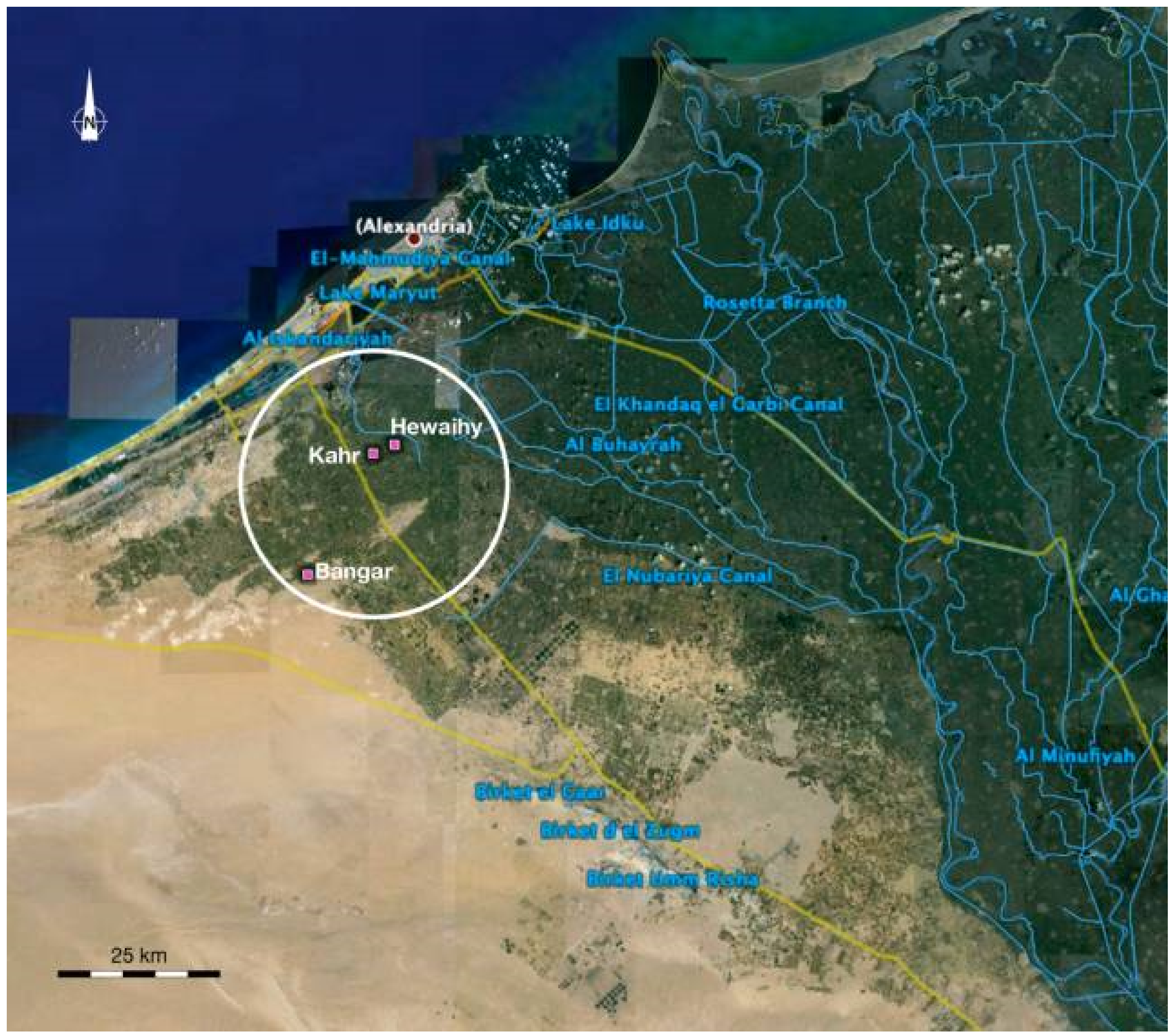
2.1. Study Site Description

The study was conducted in a region located in the southwest Nile Delta, Egypt (lat of 30.93° N and long of 29.89° E). Field work campaigns were conducted in wheat fields during the March of the winter season 2007 concurrent with satellite imagery acquisition. The field campaigns were planned to couple with the capturing time of satellite images. March time was chosen for detecting stress in wheat crops since the climate starts to be warmer over this period of time and wheat crops grow quickly. To have a spatial variation in crop health status, three study areas were selected, namely, elnaser, elkahr and elbangar covering a large area. The predominant soil of these study areas is mainly a sandy loam, since these lands have been reclaimed and cultivated recently. The climate in this region can be described as having slightly hot summers and moderate winters, with average minimum and maximum temperatures of 16.6 °C and 24.3 °C, a rainfall of 0 mm and 28.3 mm per year; humidity of 69 and 68%; and wind speed of 3.7 and 3.94 m s⁻¹. To have varying growing conditions of wheat such as healthy, water and salinity induced stress, twelve fields were selected across the entire study site (Figure 1).

Field campaigns aimed to gather ground reference data of wheat crops, which were collected randomly at different sites. All types of common irrigation systems are used across the entire study site (traditional surface, sprinkler and drip irrigation). Farmers sometimes use alternative sources of fresh water (e.g., agricultural drainage water) to irrigate crops at the tail end of the irrigation canal system, even with the risk of an increased salinity level. The canal system of delivering water into the main irrigation canals sometimes takes a longer time than usual for different reasons and thus subject crops to water stress that end up with a reduced crop productivity. Wheat is usually planted during the first and second week of November throughout the entire region and is often terminated at the beginning of May.

2.2. In Situ Spectroradiometry Measurements

In situ spectroradiometry measurements were collected from different fields across the whole study site during winter season of 2007 (7 March, 8 March and 9 March) concomitant with the collection of QuickBird satellite image. Furthermore, spectral measurements were collected in 2014 and 2015 to be used for modelling. Spectral measurements were collected from random fields across the entire study region, taking into consideration the size of the field and even the crop health status. An ASD FieldSpec mobile spectroradiometer with a spectral range of 325–1075 nm was employed to collect reflectance from wheat leaves and canopies. To keep the changes in solar zenith angle at a minimum, the spectral reflectance acquisition was restricted to between 11:00 and 15:00 h GMT. The obtained spectra were smoothed to eliminate noise at both ends of the spectrum using the ASD software, which was done for all datasets acquired by the instrument. During spectra collection, a metal stand of 2 m height was used to put the instrument at a constant distance from the ground level at all sampling locations.

2.3. Remote Sensing Imagery Acquisition, Processing and Analysis

One QuickBird image was captured covering wheat crops within the study site. QuickBird has four multi-spectral bands with a resolution of 2.4 m as high spatial resolution photography. Technical characteristics of QuickBird image of wheat fields captured is presented in

Table 1. Technical characteristics of QuickBird image of wheat fields captured on 7 March 2007 in South-West Nile Delta, Egypt.

Satellite Name	QuickBird
Acquisition date	3 July 2007
Acquisition time	09:06
Cloud cover	33%
Off nadir angle	13°
Target azimuth angle	210°
Spectral bands number	4
Environmental quality	99%
Centre location	Latitude/Longtude: 30.99°/29.84°

. The QuickBird image of wheat and other classes (e.g., clover, bare soil and water) was captured at 09:13 h GMT on 7 March 2007. The 7 March QuickBird image was radiometrically corrected by the image supplier (Infoterra Group, Newcastle upon Tyne, UK). The image to image technique in the ENVI software was run to geo-correct the image, using the previously collected ground control points (GCP) sampled for certain locations over field campaign times covering a large area of the study site. The FLAASH (Fast Line-of-sight Atmospheric Analysis of Hypercubes) module was performed to atmospherically correct the obtained image. Unsupervised and supervised classification algorithms were run in ENVI software using the corrected image to choose the most efficient algorithm for identifying wheat and other classes across the entire region. Varying unsupervised and supervised algorithms were evaluated on the acquired QuickBird image utilizing ENVI v5.1 to identify wheat, and other classes across the whole study area. Unlike unsupervised algorithms, supervised algorithms require a pre-prepared dataset collected during field campaigns. A validation dataset was constructed manually on the QuickBird image comprising more than 2000 clear pixels for every class to exclude interference between pixels of different classes (different spectral signature). Pure pixels were picked up carefully to avoid misleading data. A post classification technique, confusion matrix, was extracted for both k-means and MLC algorithms.

2.4. Sampling Strategy of Wheat Crop

During field campaigns, three random vegetative samples within each field were sampled after collecting reflectance spectra from wheat canopies to determine various wheat characteristics (LAI, plant-h, AGB and SPAD value). An area of 1 m² was sampled at the soil level and this was repeated three times within each field of the field survey. AGB was timely recorded for each sample. Wheat plant height was measured using a measuring tape. LAI is known as the ratio between the total leaf area of a certain number of sampled plants and the occupied area allocated for them. Following the calculation of the leaf area for individual samples, the LAI was calculated by the following formula:

$$\mathrm{LAI}=\frac{LA}{OA}$$

(1)

where: LAI refers to the leaf area index; LA refers to the leaf area per sample; OA is the taken land area by plants.

A hand-held SPAD 502 chlorophyll meter (Minolta, Osaka, Japan) was employed during field visits survey to measure chlorophyll concentration as SPAD values. Care was taken to measure chlorophyll relatively in apical leaves. The measures of chlorophyll were recorded at different locations on the same leaf to keep variability at a minimum, and then the average of these records was calculated.

2.5. Calculating Vegetation Spectral Indices

QuickBird has four spectral bands including blue, red, green, and infrared. Based on the sensitivity to variations in leaf pigments, aboveground biomass, leaf structure and the concentration of plant water, previously used V-SRIs were extracted from both in situ spectroradiometry data and the 7 March QuickBird image to estimate the efficiency of remote sensing and to assess the wheat characteristics. The V-SRIs were selected based on their sensitivity to changes in biomass, leaf pigmentation, leaf/tissue structure and plant water content. The indirect effects, which are manifested by changes in reflectance in the VIS and NIR ranges, are linked to leaf and canopy properties, such as leaf pigments, leaf structure, and scattering, which change as a result of stress factors.

Table 2. Formulae of tested vegetation-SRIs and references collected from previous investigations.

Vegetation-SRIs	Formulae	Reference
Difference vegetation index (DVI)	NIR − Red	[54]
Infra-Red percentage vegetation index (IPVI)	NIR/(NIR + Red)	[55]
Stress index (SI)	Red/NIR	[56]
Green normalized difference vegetation index (GNDVIbr)	(NIR − green)/(NIR + green)	[57]
Normalized difference vegetation index (NDVI)	(NIR − Red)/(NIR + Red)	[58]
Renormalized difference vegetation index (RDVI)	$\sqrt{NDVI}X DVI$	[59]
Simple ratio (SR)	NIR/Red	[60]
Specific leaf area vegetation index (SLAVI)	NIR/(Red + NIR)	[61]
Vegetation index (VI)	NIR/(green − 1)	[62]
Optimized soil adjusted vegetation index (OSAVI)	((NIR − Red)/(NIR + Red + L)) × (1 + L), L = 0.16	[63]

lists the formulae used for calculating different selected V-SRIs associated with references.

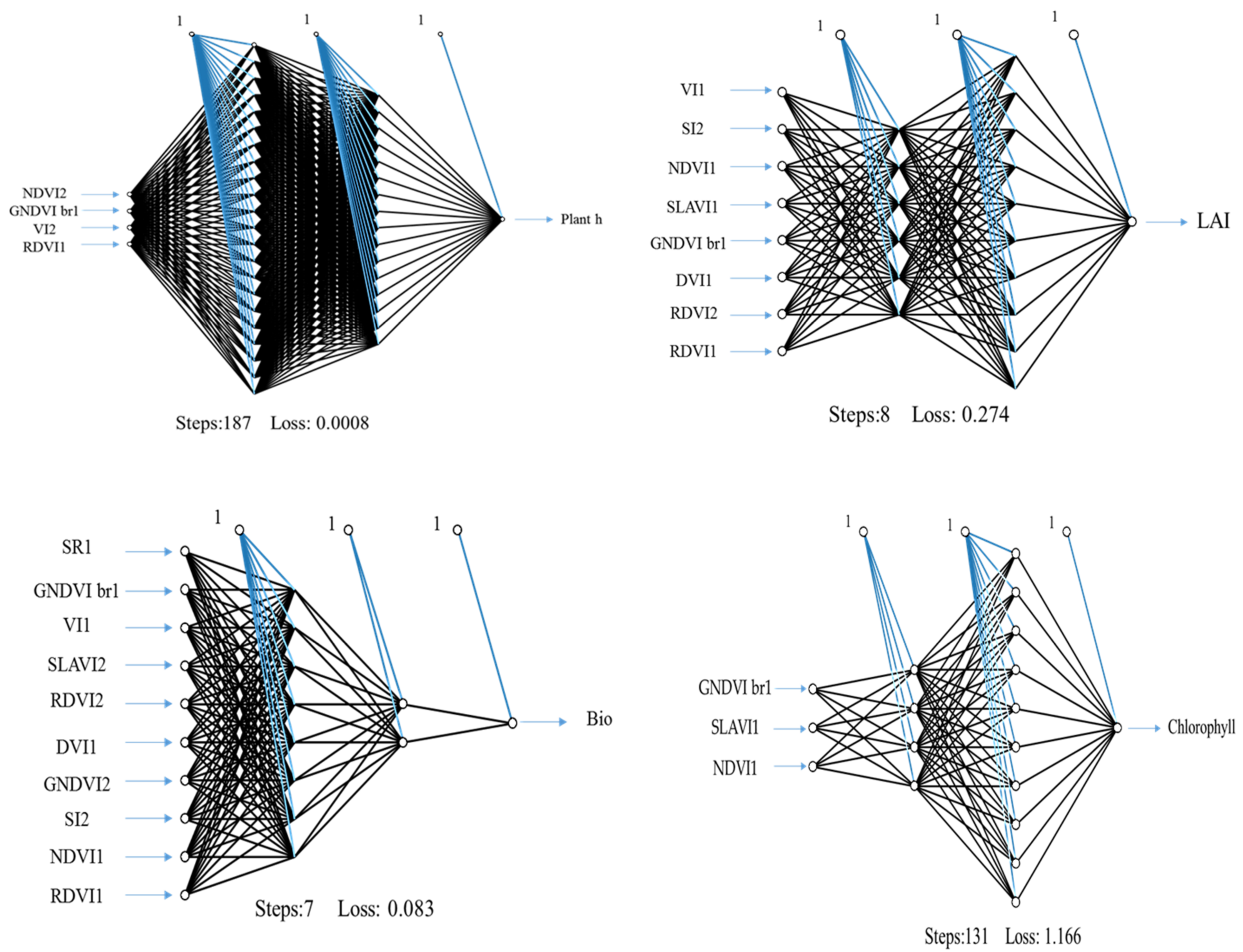
2.6. Back-Propagation Neural Network (BPNN)

One of the commonly used artificial neural networks is the BPNN [64], which is a neural network with 3 layers. The input layer of BPNN is responsible for storing the basic data of the neural network while the hidden layer is considered a connection between the first (input) and final (output) layers; the output layer is responsible for delivering the outcome of the input data. There is also a single hidden layer in the network with several nodes; the number of nodes in the hidden layer is determined by the regression’s accuracy. The hidden layer, which is often described as weight, represents the “activation” nodes. The output layer is the final layer that displays the detected value of the measured parameter. ANN models are developed as extended mathematical models that replicate human cognition in prediction and pattern recognition based on a sequence of neurons or nodes that are connected by rated connections [65,66].

The network was trained for at least 1000 iterations or until the error value dropped below a certain threshold (10⁻⁴). On the training dataset, the validation technique with the LOOV procedure was used to determine the number of neurons in the concealed layer. The restricted memory parameter of Broyden–Fletcher–Goldfarb–Shanno was chosen to efficiently implement the algorithm [67]. The formula below was used to determine the most informative feature in order to improve the predictive efficiency of the regression model and to reduce the hyperspectral image dimensionality [68].

$$\mathrm{M}=\frac{{{\displaystyle \sum }}_{j=1}^{n_H}\left[\left(\left|I\right|{ }_{P_j}/{{\displaystyle \sum }}_{k=1}^{n_p} \left|I\right|{ }_{P_{j,k}} \right){\left|O\right|}_j\right]}{{{\displaystyle \sum }}_{i=1}^{n_p}\left({{\displaystyle \sum }}_{j=1}^{n_H}\left[\left(\left|I\right|{ }_{P_{i,j}}/{{\displaystyle \sum }}_{k=1}^{n_p} \left|I\right|{ }_{P_{i,j,k}} \right){\left|O\right|}_j\right]\right)}$$

(2)

where M is a significant measure for the input variable, n_p refers to the number of variables in the input, n_H equals the number of nodes in the hidden layer, 〖|I|〗_(P_j) is the absolute value of the hidden layer weight for the pth input variable and the jth unseen layer, and |O|_j belongs to the absolute value of the output layer rating for the jth hidden layer.

2.7. Random Forest Regression (RF)

RF model, which is based on regression trees, could be a useful strategy for determining the relationship between a large number of independent variables and a single dependent variable. The RF uses the repeated partitioning method to fragment the dataset into many nodes within a homogeneous subset termed regression tree (ntree) before averaging the results of all the trees. Bootstrap sampling is then implemented based on the training dataset to build each tree to its maximum size without interrupting the input variables selection at each node. In the regression phase of each tree, the RF uses randomization by selecting a random subset of variables (mtry) for the determination of the split at each node [69]. The leave-one-out validation approach (LOOV) is then used to optimize the two major model parameters (mtry and ntree), producing a less root mean squared error of validation (RMSEV). The ntree must have a value within 1 to 25, while the value of mtry is calculated with different feature numbers. All the features were arranged once the model had been trained using the optimal parameters; the selection of the optimal features was based on the use of variable significance statistics [70]. During all iterations, the results were collected, and several options were analyzed to determine the best feature interaction, which are the ones with the lowest cost.

2.8. Model Evaluation

The statistical metrics root mean square error (RMSE) and determination coefficient (R²) were used to estimate the effectiveness of the regression model [71,72]. All parameters can be explicated by: F_act refers to the pre-determined true value which is based on laboratory calculations, F_p refers to the detected or simulated value, F_ave represents the mean value, and N represents the total number of data records.

1. Root mean square error

$$\mathrm{RMSE}=\sqrt{\frac{1}{N}{{\displaystyle \sum }}_{i=1}^N{\left(F_{act}-F_p\right)}^2}$$

(3)

2. Determination coefficient

$${\mathrm{R}}^2=\frac{{\displaystyle \sum }{\left(F_{act}-F_p\right)}^2}{{\displaystyle \sum }{\left(F_{act}-F_{ave}\right)}^2}$$

(4)

2.9. Statistical Analysis

Data were statistically analyzed using SPSS v. 12.0, (SPSS Inc., Chicago, IL, USA) and were also tested for normality by the Anderson–Darling manner at the 95% probability level. The relationship between the tested SRIs and various wheat characteristics was also investigated using simple linear regression performed in Sigma Plot v. 11.0 (SPSS, Chicago, IL, USA) to clearly identify the optimum SRIs based on the greatest value of a determination coefficient (R²). The significance level of the R² for these relationships was set at a 0.05 confidence level.

3. Results and Discussion

3.1. Effect of Well Irrigated and Varying Stress Conditions on the LAI, Plant Hight, Biomass and SPAD Value of Wheat

Data collected over different field visits demonstrated a significant difference in various wheat crop characteristics. It is obvious that salinity stress has the greatest negative impact on different crop characteristics as presented in

Table 3. Mean and standard deviation (SD) of LAI, plant height (plant-h), above ground biomass (AGB) and SPAD value of wheat crops in three years across the study site.

Fields	Field Code	Treatment	LAI	Plant-h (m)	AGB	SPAD	LAI	Plant-h (m)	AGB	SPAD	LAI	Plant-h (m)	AGB	SPAD
					(kg m−2)				(kg m−2)				(kg m−2)
			First year				Second year				Third year
Field 1	S1	Non-stress	3.85 ± 0.46 a	0.70 ± 0.05 cd	1.85 ± 0.15 b	42.2 ± 1.0 ab	3.34 ± 0.23 b	0.89 ± 0.04 ab	1.52 ± 0.02 b	43.1 ± 2.3 ab	4.30 ± 0.43 a	1.01 ± 0.01 a	2.50 ± 0.23 a	47.0 ± 1.8 a
Field 2	S2	Drought stress	2.94 ± 0.53 b	0.68 ± 0.04 de	1.39 ± 0.17 c	41.4 ± 1.7 ab	2.46 ± 0.23 de	0.87 ± 0.04 ab	1.29 ± 0.03 c	41.5 ± 1.9 b	2.82 ± 0.24 b	0.85 ± 0.04 c	1.58 b ± 0.57 c	43.5 ± 2.2 b
Field 3	S3	Drought stress	2.36 ± 0.15 b	0.86 ± 0.03 b	1.68 ± 0.07 b	43.2 ± 0.4 a	2.30 ± 0.05 ef	0.77 ± 0.08 c–e	1.17 ± 0.06 d	41.1 ± 1.9 b	2.54 ± 0.33 b	0.84 ± 0.07 c	1.18 ± 0.55 cd	41.4 ± 0.6 bc
Field 4	S4	Drought stress	2.55 ± 0.56 b	0.75 ± 0.08 c	1.4 ± 0.16 bc	41.6 ± 0.4 ab	2.76 ± 0.19 cd	0.84 ± 0.06 bc	1.44 ± 0.04 b	42.7 ± 0.4 b	2.36 ± 0.24 b	0.68 ± 0.07 d	1.14 ± 0.54 cd	39.7 ± 1.0 c
Field 5	S5	Drought stress	2.81 ± 0.25 b	0.65 ± 0.04 de	0.97 ± 0.04 d	41.1 ± 0.2 ab	2.81 ± 0.10 c	0.78 ± 0.06 cd	1.42 ± 0.03 b	41.1 ± 0.2 b	2.82 ± 0.24 b	0.85 ± 0.04 c	1.66 ± 0.46 bc	42.8 ± 2.3 bc
Field 6	KO	Non-stress	4.09 ± 0.42 a	1.00 ± 0.03 a	2.2 ± 0.24 a	44.9 ± 1.0 a	3.85 ± 0.47 a	0.95 ± 0.04 a	1.69 ± 0.09 a	45.5 ± 0.5 a	4.00 ± 0.42 a	1.03 ± 0.02 a	2.34 ± 0.09 ab	43.6 ± 0.6 b
Field 7	RA	Non-stress	4.03 ± 0.43 a	1.013 ± 0.01 a	1.98 ± 0.07 a	44.6 ± 2.9 a	3.09 ± 0.16 bc	0.89 ± 0.06 ab	1.50 ± 0.01 b	43.3 ± 0.9 ab	2.85 ± 0.23 b	0.69 ± 0.18 d	1.60 ± 0.63 bc	41.2 ± 2.2 bc
Field 8	ME	Non-stress	4.0 ± 0.42 a	1.03 ± 0.02 a	2.03 ± 0.10 a	42.6 ± 1.6 a	2.94 ± 0.19 c	0.90 ± 0.05 ab	1.44 ± 0.05 b	43.2 ± 1.4 ab	2.85 ± 0.28 b	0.97 ± 0.02 ab	1.66 ± 0.63 bc	42.1 ± 1.6 bc
Field 9	TA	Salinity stress	1.98 ± 0.61 c	0.89 ± 0.04 b	0.94 ± 0.21 e	36.0 ± 3.3 bc	2.12 ± 0.10 e–g	0.78 ± 0.02 cd	1.03 ± 0.03 e	38.5 ± 0.5 c	0.76 ± 0.05 d	0.62 ± 0.01 de	0.32 ± 0.03 e	29.2 ± 2.0 f
Field 10	SH	Salinity stress	2.85 ± 0.05 cd	0.67 ± 0.02 de	1.10 ± 0.03 f	32.7 ± 1.9 c	2.00 ± 0.18 fg	0.73 ± 0.04 de	0.97 ± 0.09 e	36.5 ± 1.3 c	1.42 ± 0.60 c	0.89 ± 0.04 bc	0.61 ± 0.22 de	36.0 ± 3.3 d
Field 11	OMA	Salinity stress	2.15 ± 0.11 d	0.53 ± 0.06 f	1.32 ± 0.01 f	23.7 ± 2.0 d	1.57 ± 0.11 h	0.73 ± 0.06 de	0.72 ± 0.11 f	31.8 ± 1.5 d	1.06 ± 0.05 cd	0.67 ± 0.02 d	0.49 ± 0.13 de	32.7 ± 1.9 e

The values having same letters are non-statistically significant (p ≤ 0.05) among different fields.

. LAI values differed from 2.85 to 4.09 for non-stress, varied from 2.30 to 2.94 for drought stress, and varied from 0.67 to 2.85 for salinity stress across three years (Table 3). Broadly, the obtained results demonstrated the spatial distribution of different wheat characteristics with, values of the LAI varying from 2.85 to 4.09; BFW varying from 0.25 to 2.5 kg m⁻²; Plant-h varying from 0.53 to 1.03 m and SPAD values varying from 22.4 to 47.0 as an indicator of total chlorophyll concentration (Table 3), across three years.

The results further showed that salinity stress had the highest impact on different crop characteristics followed by water stress, as detailed in Table 3. The noticeable variations in LAI, plant-h, AGB, and SPAD values between non-stress, drought stress, and salinity stress wheat may be attributed to various photosynthetic activities that are closely related to the development of leaves and aerial fresh biomass. The adverse effect of both parameters can lead to impaired necessary development processes. Salinity is among the most negatively influencing parameter of productivity and quality of wheat through the changing biochemical and physiological main activities in crops [73]. It also delays the seedling germination, inhibits the growth of seedlings, and seedling metabolism lead to a decreased plant growth and final crop yield [74]. Additionally, salinity negatively impacts the growth and thus the final yield of crops through reducing the available soil moisture in the rootzone, and also the toxic effects of high concentrations of both chloride and sodium ions to plants [75]. Moreover, salinity reduces the number of fertile tellers, kernel weight and the number of spikelets per spike (Abass et al., 2013), decreases the number of grains per spike, to a 1000 grain weight [76] and finally leads to less productivity [77]. The salinity stress remarkably affected the measured characteristics of corn in comparison to the other factors. Salinity inhibits leaf initiation and elongation, as well as internode advancement, and accelerates leaf abscission, resulting in lower BFW and LAI [20,21]. Salinity stress reduces photosynthetic pigments such as chlorophylls a and b, as well as carotenoids, which are linked to a poor net photosynthesis rate in maize [21]. These findings support the need for a regular and timely evaluation of the assessed cop traits in order to improve wheat tolerance to changing stress situations. As a result, boosting wheat tolerance necessitates large-scale techniques (e.g., remote sensing of different platforms) that are dependable, rapid, and non-destructive.

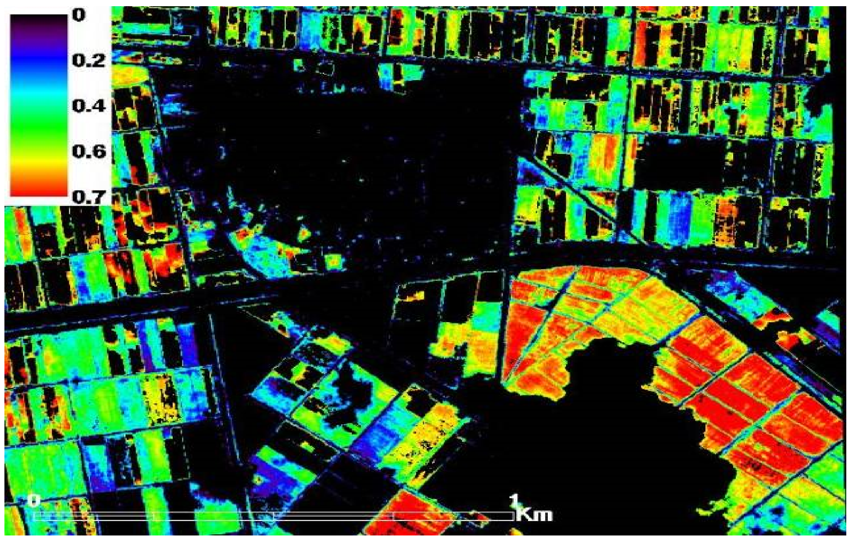
3.2. Satellite-Based NDVI for Well-Irrigated and Stressed Wheat Fields

During fieldwork campaigns across the three study sites, twelve different fields were chosen randomly, taking into consideration the crop health status to have a range of healthy wheat fields and varying stress conditions (e.g., drought and salinity stress) to spot the spatio-temporal variations in the records of LAI, plant-h, AGB and SPAD values of the wheat crop. Obvious differences in values of the measured wheat characteristics were noticed. As seen in Figure 2 as an example of satellite-based NDVI for non-stress and stressed wheat fields. The observed healthy wheat fields (red in color) receive the same agricultural practices (e.g., planting date, fertilization dose, same wheat cultivar and irrigation regimes). Stressed wheat fields, seen in the top right corner of the image, are lacking freshwater resources since they are at the tail end of the irrigation network and therefore wheat crops suffer from either water or salinity stress caused from using agricultural drainage water as an alternative water source to canal fresh water. Generally, this area is influenced by high salinity stress since it has been irrigated with highly saline-water (water salinity > 4 dS m⁻¹) for more two decades. Figure 2 also shows a gradient in NDVI records in the healthy location, which may have been a result of moderate moisture stress. Moreover, the efficiency of the drainage system may vary from one field to another in the neighboring fields (small-field system) depending on how far the ditches are, which in turn affect the availability of water for plants.

3.3. Classifying Wheat and Other Crops across the Study Area

As presented in

Table 4. Outputs of confusion matrix for MLC of wheat and other classes in the south-west Nile Delta, Egypt.

Class	Ground Truth (%)					User’s Accuracy
	Wheat	Water	Soil	Clover	Total
Wheat	90.4	0.00	2.0	1.3	22.8	96.3
Water	4.3	97.8	1.5	1.7	25.7	96.9
Soil	5.3	2.1	92.5	11.1	28.9	84.5
Clover	0.00	0.1	4.0	86.0	22.6	90.7
Total	100	100	100	100	100.0
Producer’s Accuracy (%)	90.4	97.8	92.5	86.0
Kappa Coefficient	0.90
Overall Accuracy (%)	91.7

, MLC algorithms produced four different classes mainly wheat, water surfaces, clover, and soil. As a post-classification technique, a confusion matrix was built up to assess various classification algorithms providing the total accuracy, accuracy for single class, kappa coefficient, producer’s and user’s accuracies. The obtained results demonstrated a high accuracy for classifying different classes ranging between 86.0% for classifying clover and 97.8% for classifying water. The same trend was observed for both producer’s and user’s accuracies, since they were also high in MLC algorithm (>0.84). It can also be observed that the accuracy for determining wheat crops using MLC was greater than 0.90%, along with high accuracies for categorizing other classes (Table 4).

Unlike supervised algorithms, k-means does not require a reference dataset. Although k-means gave high classification accuracy for wheat and clover as the two main cultivated crops in the winter across the study area throughout the image (97.6% and 94.6%) as presented in

Table 5. Outputs of confusion matrix extracted for the k-means classifier of wheat and other classes in the study area South-West Nile Delta, Egypt.

Class	Ground Truth (%)					User’s Accuracy
	Wheat	Water	Soil	Clover	Total
Wheat	97.6	25.7	12.7	4.2	35.1	69.9
Water	2.0	72.5	45.1	0.3	29.4	61.7
Soil	0.4	1.3	42.2	1.9	10.4	96.1
Clover	0.00	1.5	0.00	94.6	25.1	98.6
Total	100	100	100	100	100.0
Producer’s Accuracy (%)	97.6	72. 5	42.2	94.6
Kappa Coefficient	0.70
Overall Accuracy	77.40%

, a lesser accuracy for identifying water and soil surfaces is clear, which may lead to a greater number of misclassified pixels and thus produced a lesser overall accuracy. K-means outputs produced a high accuracy for classifying wheat crops across the study area, but in the meantime, the total accuracy for identifying individual classes are less when compared with MLC. Furthermore, the Kappa coefficient for MLC was higher (0.90) compared with that obtained value from the k-means algorithm (0.70), which can be attributed to great number of misclassified pixels. One source of misclassified pixels is the interference between dry bare soils and wet bare soils, which varied in reflecting solar energy. The results therefore suggested that the MLC classifier produced a higher total accuracy and single classification accuracies, as well for classifying various crops throughout the entire study area.

3.4. Assessment of Various Vegetation-SRIs Derived from Both In Situ Spectroradiometry and Satellite Based Remote Sensing Data under Non-Stress and Stress Conditions

The SRIs calculated from different fields throughout the study site showed high effectiveness in assessing wheat crop characteristics including LAI, plant-h, AGB and SPAD value. The spectra collected on different dates were combined to choose the optimum indices for the detection of wheat characteristics. As an indicator for the relationship between wheat characteristics and SRIs, the coefficient of determination (R²) showed strong relationships. The results demonstrated that most of the SRIs derived from in situ spectral measurements produced high correlations with the measured wheat characteristics with R² values reaching up to 0.85 for the detection of different wheat characteristics (

Table 6. Coefficient of determination for the association between various vegetation-SRIs obtained from in situ spectroradiometry and Egyptian wheat characteristics in three years, collected from the study site.

Vegetation Index	Crop Properties
	LAI	Height (m)	Biomass (kg·m−2)	SPAD
		0.23 *	0.53 ***	0.46 **
DVI	0.58 ***	0.25 *	0.58 ***	0.61 ***
IPVI	0.61 ***	0.21	0.61 ***	0.52 **
SI	0.65 ***	0.23 *	0.55 ***	0.48 **
GNDVI	0.65 ***	0.28 *	0.61 ***	0.62 ***
NDVI	0.67 ***	0.21	0.53 ***	0.50 **
RDVI	0.59 ***	0.23 *	0.54 ***	0.49 **
SR	0.61 ***	0.18	0.48 **	0.53 ***
SLAVI	0.52 **	0.16	0.51 **	0.52 **
VI	0.60 ***	0.20	0.55 ***	0.41 ***

Levels of significance: *: p-value < 0.05, **: p-value < 0.01, and ***: p < 0.001.

). SRIs were presented as having moderate to strong relationships with LAI and AGB, and R² varied from 0.54 to 0.84 and R² varied from 0.47 to 0.85, respectively. Interestingly, RDVI extracted from in situ measurements was shown to be the most sensitive index for assessing LAI, and AGB with respective R² values of 0.84, and 0.85 across three years. SRIs were presented as having low to moderate relationships, with plant-h with R² varying from 0.16 to 0.59. The highest relationships were found between IPVI and NDVI and plant-h, with R² = 0.59 at the second year. SRIs were presented moderate to strong relationships with chlorophyll (SPAD values) with R² varied from 0.39 to 0.82. The IPVI, NDVI, and SLAVI were the optimum indices for the detection of chlorophyll (SPAD values) with an R² of 0.82 at first year (Table 6). The results further showed the effectiveness of QuickBird satellite images in detecting wheat characteristics. The SRIs derived from the satellite image showed good relationships with three wheat characteristics (AGB, LAI and SPAD value) and R² values varied from 0.51 to 0.61; 0.52 to 0.67, and 0.41 to 0.61 respectively. The NDVI derived from the satellite data was shown to be the most sensitive index for assessing AGB, LAI and chlorophyll (

Table 7. Coefficient of determination for the association between various vegetation-SRIs obtained from QuickBird satellite image and Egyptian wheat characteristics collected from the study site.

Vegetation Index	Crop Properties
	LAI	Height	AGB	SPAD	LAI	Height	AGB	SPAD	LAI	Height	AGB	SPAD
	First year				Second year				Third year
DVI	0.74 ***	0.40 **	0.77 ***	0.58 ***	0.64 ***	0.57 ***	0.73 ***	0.46 ***	0.74 ***	0.32 ***	0.68 ***	0.65 ***
IPVI	0.75 ***	0.42 **	0.79 ***	0.82 ***	0.65 ***	0.59 ***	0.77 ***	0.52 ***	0.72 ***	0.42 ***	0.64 ***	0.75 ***
SI	0.68 ***	0.38 **	0.72 ***	0.80 ***	0.62 ***	0.58 ***	0.74 ***	0.51 ***	0.65 ***	0.39 ***	0.57 ***	0.72 ***
GNDVI	0.70 ***	0.45 **	0.71 ***	0.65 ***	0.67 ***	0.54 ***	0.74 ***	0.46 ***	0.59 ***	0.30 ***	0.57 ***	0.56 ***
NDVI	0.75 ***	0.42 **	0.78 ***	0.82 ***	0.65 ***	0.59 ***	0.77 ***	0.52 ***	0.72 ***	0.42 ***	0.64 ***	0.75 ***
RDVI	0.84 ***	0.51 **	0.85 ***	0.70 ***	0.70 ***	0.50 ***	0.77 ***	0.50 ***	0.83 ***	0.46 ***	0.75 ***	0.71 ***
SR	0.82 ***	0.53 ***	0.82 ***	0.61 ***	0.68 ***	0.44 ***	0.72 ***	0.47 ***	0.79 ***	0.43 ***	0.72 ***	0.62 ***
SLAVI	0.75 ***	0.42 **	0.79 ***	0.82 ***	0.65 ***	0.59 ***	0.77 ***	0.52 ***	0.72 ***	0.42 ***	0.64 ***	0.75 ***
VI	0.62 ***	0.26 *	0.65 ***	0.39 ***	0.67 ***	0.45 ***	0.70 ***	0.44 ***	0.54 ***	0.16 ***	0.47 ***	0.49 ***
OSAVI	0.78 ***	0.42 **	0.81 ***	0.77 ***	0.72 ***	0.61 ***	0.81 ***	0.54 ***	0.75 ***	0.40 ***	0.66 ***	0.75 ***

Levels of significance: *: p-value < 0.05, **: p-value < 0.01, and ***: p < 0.001.

). The NDVI included with VIS and NIR wavebands was widely recommended for assessing biophysical properties (biomass, LAI, and green vegetation cover) [78,79]. All the SRIs derived from the satellite image showed weak relationships, with a wheat plant height. The difference in R² values produced from in situ spectra and satellite data could be due to the time difference between collecting the vegetation sample and the acquisition of satellite images. The satellite image was captured a few days prior to the field surveys, while the spectroradiometry campaigns were concurrent with collecting vegetation samples; this explains why R² values for the SRIs extracted from in situ data had higher correlations with the measured wheat characteristics. Many previous studies employed ground and satellite-based vegetation-SRIs which agree with our findings in terms of assessing plant growth and SPAD value performance [78,79,80,81,82,83,84]. For example, Gao et al. [80] discovered that four maize plant growth parameters and SRIs had positive correlation coefficients: the ratio vegetation index (RVI) for the LAI (r = 0.47), biomass (r = 0.59), height (r = 0.59), and leaf water area index (LWAI) (r = 0.54). For these variables, Towers et al. [85] found that the NDVI and Enhanced Vegetation Index (EVI) showed similar correlation coefficients. The NDVI showed a closer relationship with LAI than the perpendicular (PVI), mixed soil-adjusted vegetation index 2 (SAVI2) and modified soil-adjusted vegetation indices (MSAVIs) and the chlorophyll index (CIrededge). The findings of this study revealed that ground remote-sensing and satellite imagery have the possibility to provide critical crop monitoring data in irrigated and stressed areas.

The differences observed between the values of R² in Table 6 and Table 7 may be due to; (1) the time difference between collecting in situ spectra data and satellite acquisition time; (2) another reason is that in situ spectra are collected at the nadir position, while satellite images are not; and (3) spectroradiometers have an accuracy of 1 nm, while the QuickBird satellite has a resolution of 2 m, which can affect the derivation of different indices.

3.5. Performance Evaluation of Various Models to Detect the Measured Wheat Characteristics

In the present investigation, the two groups of SRIs (group1, SRIs of in situ spectrometry and group2, SRIs of satellite imagery) were used in a single or a combined form as input variables in the ANN and RF, to assess the four measured wheat parameters In

Table 8. Outcomes of calibration and validation models of ANN for the association between V-SRIs extracted from in situ spectrometry and satellite imagery and leaf area index, plant height, above ground biomass and SPAD value prior selecting the best features.

Variables	Group	Parameters	Training		Validation
			R2	RMSE	R2	RMSE
LAI	Group 1	(8, 16) & relu	0.87 ***	0.127	0.84 ***	0.135
	Group 2	(16, 8) & tanh	0.97 ***	0.108	0.62 ***	0.226
	Total	(2, 20) & relu	0.99 ***	0.080	0.93 ***	0.122
Plant-h	Group 1	(2, 4) & logistic	0.66 ***	0.084	0.50 ***	0.099
	Group 2	(16, 6) & relu	0.83 ***	0.068	0.26 **	0.115
	Total	(6, 22) & relu	0.81 ***	0.071	0.28 **	0.108
AGB	Group 1	(2, 2) & tanh	0.87 ***	0.222	0.79 ***	0.214
	Group 2	(10, 22) & relu	0.84 ***	0.271	0.77 ***	0.231
	Total	(2, 20) & relu	0.96 **	0.181	0.71 ***	0.266
SPAD value	Group 1	(2, 22) & tanh	0.89 ***	1.251	0.76 ***	2.065
	Group 2	(4, 6) & logistic	0.94 ***	1.051	0.32 **	3.859
	Total	(2, 20) & relu	0.93 ***	1.069	0.71 ***	2.169

Levels of significance: **, ***: at p < 0.01, and p < 0.001, respectively. Group 1, SRIs extracted from in situ spectrometry. Group 2, SRIs extracted from satellite imagery.

,

Table 9. Outcomes of calibration (n = 96) and validation models (n = 48) of ANN for the association between the best V-SRIs extracted from in situ spectrometry and satellite imagery and leaf area index, Plant height, above ground biomass and SPAD value.

Variables	Best Indices	Parameters	Training		Validation
			R2	RMSE	R2	RMSE
LAI	VI1, SI2, NDVI1, SLAVI1, GNDVI br1, DVI1, RDVI2, RDVI1	(6, 10) & relu	0.99 ***	0.067	0.97 ***	0.109
Plant-h	NDVI2, GNDVI br1, VI2, RDVI1	(22, 16) & relu	0.94 ***	0.023	0.72 ***	0.039
AGB	SR1, GNDVI br1, VI1, SLAVI2, RDVI2, DVI1, GNDVI2, SI2, NDVI1, RDVI1	(8, 2) & relu	0.94 ***	0.104	0.87 ***	0.112
SPAD value	GNDVI br1, SLAVI1, NDVI1	(4, 10) & relu	0.90 ***	1.336	0.86 ***	1.275

1 refers to the SRIs extracted from in situ spectrometry and 2 refers to the SRIs extracted from satellite imagery. Levels of significance: ***: p < 0.001. n is number of samples which used in calibration and validation models.

,

Table 10. Outcomes of calibration and validation models of random forest for the association between V-SRIs extracted from in situ spectrometry and satellite imagery and leaf area index, plant height, above ground biomass and SPAD value before selecting the best features.

Variables	Group	Parameters	Training		Validation
			R2	RMSE	R2	RMSE
LAI	Group 1	ntree = 3, mtry = 20	0.97 ***	0.203	0.82 ***	0.317
	Group 2	ntree = 4, mtry = 6	0.92 ***	0.245	0.66 ***	0.325
	Total	ntree = 13, mtry = 6	0.98 ***	0.099	0.91 ***	0.179
Plant-h	Group 1	ntree = 5, mtry = 8	0.82 ***	0.060	0.51 ***	0.070
	Group 2	ntree = 2, mtry = 7	0.73 ***	0.086	0.26 *	0.108
	Total	ntree = 7, mtry = 7	0.90 ***	0.031	0.60 ***	0.048
AGB	Group 1	ntree = 8, mtry = 21	0.96 ***	0.108	0.82 ***	0.194
	Group 2	ntree = 22, mtry = 8	0.90 ***	0.119	0.51 ***	0.313
	Total	ntree = 9, mtry = 8	0.97 ***	0.073	0.80 ***	0.137
SPAD value	Group 1	ntree = 2, mtry = 11	0.93 ***	1.628	0.68 ***	2.192
	Group 2	ntree = 25, mtry = 3	0.90 ***	2.545	0.45 **	4.601
	Total	ntree = 2, mtry = 6	0.97 ***	0.777	0.74 ***	1.544

Levels of significance: *, **, ***: at p < 0.05, p < 0.01, and p < 0.001, respectively. Group 1, SRIs extracted from in situ spectrometry. Group 2, SRIs extracted from satellite imagery.

and

Table 11. Outcomes of calibration (n = 96) and validation models (n = 48) of random forest for the association between the best V-SRIs extracted from in situ spectrometry and satellite imagery and leaf area index, plant height, above ground biomass and SPAD value.

Variables	Best Indices	Parameters	Training		Validation
			R2	RMSE	R2	RMSE
LAI	IPVI1, RDVI1, DVI1, RDVI2, SR1, OSAVI1	ntree = 3, mtry = 4	0.96 ***	0.149	0.93 ***	0.161
Plant-h	DVI1, NDVI2, SR1	ntree = 2, mtry = 11	0.91 ***	0.029	0.64 ***	0.044
AGB	IPVI2, RDVI2, NDVI1, RDVI1, SR1, DVI1, OSAVI1	ntree = 4, mtry = 10	0.96 ***	0.083	0.81 ***	0.126
SPAD value	SR1, NDVI2, VI1, SLAVI1, SI2, DVI1, OSAVI1, RDVI1, SR2, RDVI2, IPVI2, SI1, IPVI1, NDVI1	ntree = 2, mtry = 16	0.96 ***	0.874	0.75 ***	1.605

1 refers to the SRIs extracted from in situ spectrometry and 2 refers to the SRIs extracted from satellite imagery. Levels of significance: ***: p < 0.001.

. These indices showed a high performance for identifying the tested crop characteristics. Both models of ANN and RF of in situ spectroradiometry were tested using the two-year datasets as calibration datasets (n = 72) and validation datasets (n = 36). Both models of ANN and RF of high resolution satellite images were tested using the two-year datasets as calibration datasets (n = 24) and validation datasets (n = 12). As well as this, both models of ANN and RF combining data from ANN and RF of in situ spectroradiometry and high resolution satellite images were tested using the two year datasets as calibration datasets (n = 96) and validation datasets (n = 48).

The ANN and RF were trained using the V-SRIs of ground-based, satellite-based remote sensing and all indices as independent variables for detecting the tested characteristics of wheat (dependent inputs) as presented in Table 8 and Table 10. The results revealed that the ground–satellite indices (GSIs) were the outstanding integration to separate the topmost variables, as shown in Table 9 and Table 11. A comparison between the predictable values and the reserved values was conducted, which was not implemented for the ANN. Our investigation aimed to evaluate machine-learning approach performance and then compare the outputs clearly, so that the use of this model remarkably enhances predictability. Independent validation is the most optimal way for evaluating the efficiency of the regression model because validation datasets are not used in the model construction process. According to its performance, the ANN-GSIs-8 was the top detective model, resulting in a stronger link between complex features and LAI (Table 9, Figure 3). The three features of V-SRIs of both methods comprised in such model are of considerable significance for estimating LAI. It generated an R² value of 0.99 and 0.97 for the training and validation datasets, respectively. Regarding the plant-h identification performance, the ANN-GSIs-4 model outperformed the other models. The R² value for the training dataset was 0.94, while that of the validation dataset was 0.72 as seen in Table 9. The achieved R² values of 0.94 and 0.87 for the training and validation datasets, respectively, portrayed the ANN-GSIs-10 as the most accurate AGB prediction model in this study. Table 9 shows the ANN-GSIs-8 model that was developed for determining chlorophyll in plants; the performance of this model exceeded the expectations, as it achieved the R² value of 0.90 and 0.86 for the training and validation datasets, respectively. Elsherbiny et al. [48] suggested that despite the improvement in the expected performance, there is a need for more actions during the training process to upgrade the regression models for better predictions; such actions may include the separation of the high-level features, and optimization of the model hyperparameters. Similar to our results, Kizil et al. [86] found that ANNs based on the NDVI, SR, green NDVI, chlorophyll green (CLg), red NDVI, and chlorophyll red edge (CLr) indices have a high potential for predicting lettuce yield under drought stress.

The performance of the RF models was compared based on the ground–satellite indices, integrating all the studied indices as shown in Table 10. This Table illustrates the best proposed indices, best parameters, and model outputs for RMSE, and R² via training, and validation set. Outcomes of advanced models after adopting the best features were optimized, as explained in Table 11. The RF-GSIs-6 model was superior in the prediction of LAI and was built with 3 (ntree: number of trees) and 4 (mtry: number of features). This model enhanced R², and RMSE to 0.93, and 0.161, respectively. The RF-GAI-3 model achieved a high expectation at 2 ntree and 11 mtry for forecasting plant-h (Table 11). The performance rose to 0.64 and 0.044 for R², and RMSE, respectively. The RF-GSIs-7 model was established through 4ntree and 10 ntry to estimate AGB. The R² increased to 0.81, while RMSE decreased to 0.126. At RF-GSIs-14 model, the validation at ntree of 2 and mtry of 16 was optimized by 14 indices. Model behavior improved with R² (0.75), and RMSE (1.605), respectively in Table 11. The proposed RF models achieved high performance by following some procedures; optimizing hyperparameters and selecting the best indices [87]. Recently, some investigations have concluded that the SRIs concurrent with the promotion of different machine-learning models would be useful for improving the detection of plant characteristics in comparison to the use of individual SRIs [48,50,52,53,88]. For example, Yang et al. [52] found that the optimized V-SRIs were more reasonable as input parameters in the RF models and some previously published SRIs (e.g., NDVI, MSAVI, and SRVI), in estimating the biomass of potato and corn crops. These findings show that selecting the appropriate SRIs as input variables in various models is critical to the models’ performance in determining crop characteristics. Both ANN and RF seem to be potential tools for predicting the measured crop traits using the integrated SRIs from ground-based remote sensing and satellite imagery. The ANN model provides a step forward to increase the predictability of measured crop characteristics, more than RF and SRIs.

The results suggested that robust prediction accuracy for the proposed variables could be achieved if a suitable algorithm and higher variables were assigned. Compared to previous research, Song et al. [89] explained that the ANNs and SVMs do not have significant differences in classification accuracy, but the SVM usually performs slightly better. The SVM classifier has a greater tolerance on a small training set and avoids the problem of insufficient training of ANN classifiers. The ANNs and SVMs can vary greatly with regards to training time. Salas et al. [90] showed that the Maximum Entropy (MaxEnt) and Generalised Linear Model (GLM) had strong discriminatory image classification abilities, with area under-the-curve (AUC) values ranging between 0.75 and 0.93 for MaxEnt and between 0.73 and 0.92 for GLM. The ensemble model resulted in improved accuracy scores compared to individual models. In this work, the advanced models were performed more accurately than the previous researchers due to the optimization of hyperparameters and the selection of different high-level features.

4. Conclusions

This research work aimed to assess the effectiveness of in situ spectroradiometry and satellite-based remote sensing data as robust and reliable approaches in site-specific management in both arid and semi-arid environments. In our research, we evaluated the performance of V-SRIs obtained from both in situ spectroradiometry measurements and high resolution QuickBird images to quantify LAI, plant-h, AGB, and SPAD values of wheat across healthy, water and salinity-induced stress in the Nile Delta region. The main results obtained from the presented research indicated that most of vegetation-SRIs extracted from the two platforms could effectively assess wheat characteristics. Generally, the vegetation-SRIs of spectrometry data demonstrated a greater R² with the measured wheat traits in comparison with the vegetation-SRIs obtained from QuickBird data. Overall, both in situ spectroradiometry and satellite-based indices showed a high performance for detecting the measured wheat characteristics. Both ANN and RF seem to be potential tools for predicting the measured crop traits using the integrated SRIs from in situ spectroradiometry and remote sensing satellite images. The ANN model offers an advantageous tool to increase the prediction efficiency of measured crop characteristics more than RF and spectral indices. For example, the ANN-GSIs-3 model constructed for the determination of chlorophyll in the plant, which had higher performance expectations (R² = 0.96 and 0.92 for training and validation datasets, respectively). In conclusion, both ANN and RF models are simple, accurate, reliable and would be highly efficient in non-destructive and large-scale methods to detect different plant morpho-physiological characteristics quickly and precisely, especially with the new advances in satellite imagery technology.

References

1. Chen, S.; Zhang, X.; Shao, L.; Sun, H.; Liu, X. Effect of deficit irrigation with brackish water on growth and yield of winter wheat and summer maize. Chin. J. Eco-Agric. 2011, 19, 579–585. [Google Scholar] [CrossRef]
2. Darko, E.; Janda, T.; Majláth, I.; Szopkó, D.; Dulai, S.; Molnár, I.; Türkösi, E.; Molnár-Láng, M. Salt stress response of wheat–barley addition lines carrying chromosomes from the winter barley “Manas”. Euphytica 2014, 203, 491–504. [Google Scholar] [CrossRef] [Green Version]
3. El-Hendawy, S.; Elsayed, S.; Al-Suhaibani, N.; Alotaibi, M.; Tahir, M.U.; Mubushar, M.; Attia, A.; Hassan, W.M. Use of hyperspectral reflectance sensing for assessing growth and chlorophyll content of spring wheat grown under simulated saline field conditions. Plants 2021, 10, 101. [Google Scholar] [CrossRef] [PubMed]
4. Elsayed, S.; Rischbeck, P.; Schmidhalter, U. Comparing the performance of active and passive reflectance sensors to assess the normalized relative canopy temperature and grain yield of drought stressed barley cultivars. Field Crops Res. 2015, 177, 148–160. [Google Scholar] [CrossRef]
5. Jones, H.G. Use of infrared thermometry for estimation of stomatal conductance as a possible aid to irrigation scheduling. Agric. For. Meteorol. 1999, 95, 139–149. [Google Scholar] [CrossRef]
6. Elmetwalli, A.H.; Tyler, A.N.; Moghanm, F.S.; Alamri, S.A.M.; Eid, E.M.; Elsayed, S. Integration of radiometric ground-based data and high-resolution QuickBird imagery with multivariate modeling to estimate maize traits in the Nile Delta of Egypt. Sensors 2021, 21, 3915. [Google Scholar] [CrossRef]
7. Zhang, F.; Zhou, G. Estimation of vegetation water content using hyperspectral vegetation indices: A comparison of crop water indicators in response to water stress treatments for summer maize. BMC Ecol. 2015, 19, 18. [Google Scholar] [CrossRef] [Green Version]
8. Ge, Y.; Atefi, A.; Zhang, H.; Miao, C.; Ramamurthy, R.K.; Sigmon, B.; Yang, J.; Schnable, J.C. High-throughput analysis of leaf physiological and chemical traits with VIS–NIR–SWIR spectroscopy: A case study with a maize diversity panel. Plant Methods 2019, 15, 66. [Google Scholar] [CrossRef] [Green Version]
9. Elmetwalli, A.H.; El-Hendawy, S.E.; Al-Suhaibani, N.; Alotaibi, M.; Tahir, M.U.; Mubushar, M.; Hassan, W.M.; El-Sayed, S. Potential of hyperspectral and thermal proximal sensing for estimating growth performance and yield of soybean exposed to different drip irrigation regimes under arid conditions. Sensors 2020, 20, 6569. [Google Scholar] [CrossRef]
10. Babar, M.A.; Reynolds, M.P.; van Ginkel, M.; Klatt, A.R.; Raun, W.R.; Stone, M.L. Spectral reflectance to estimate genetic variation for in-season biomass, leaf chlorophyll, and canopy temperature in wheat. Crop Sci. 2006, 46, 1046–1057. [Google Scholar] [CrossRef]
11. Jin, X.; Yang, G.; Xu, X.; Yang, H.; Feng, H.; Li, Z.; Shen, J.; Lan, Y.; Zhao, C. Combined multi-temporal optical and radar parameters for estimating LAI and biomass in winter wheat using HJ and RADARSAR-2 data. Remote Sens. 2015, 7, 13251–13272. [Google Scholar] [CrossRef] [Green Version]
12. Rischbeck, P.; Elsayed, S.; Mistele, B.; Barmeier, G.; Heil, K.; Schmidhalter, U. Data fusion of spectral, thermal and canopy height parameters for improved yield prediction of drought stressed spring barley. Eur. J. Agron. 2016, 78, 44–59. [Google Scholar] [CrossRef]
13. Rischbeck, P.; Baresel, P.; Elsayed, S.; Mistele, B.; Schmidhalter, U. Development of a diurnal dehydration index for spring barley phenotyping. Funct. Plant Biol. 2014, 41, 12. [Google Scholar] [CrossRef]
14. Poss, J.A.; Russell, W.B.; Grieve, C.M. Estimating yield of salt-and water-stressed forages with remote sensing in the visible and near infrared. J. Environ. Qual. 2006, 35, 1060–1071. [Google Scholar] [CrossRef] [Green Version]
15. Hackl, H.; Mistele, B.; Hu, Y.; Schmidhalter, U. Spectral assessments of wheat plants grown in pots and containers under saline conditions. Funct. Plant Biol. 2013, 40, 409–424. [Google Scholar] [CrossRef]
16. Mansour, E.; Moustafa, E.S.A.; Desoky, E.M.; Ali, M.M.A.; Yasin, M.A.T.; Attia, A.; Alsuhaibani, N.; Tahir, M.U.; El-Hendawy, S.E. Multidimensional evaluation for detecting salt tolerance of bread wheat genotypes under actual saline field growing conditions. Plants 2020, 9, 1324. [Google Scholar] [CrossRef]
17. Hirich, A.; Fatnassi, H.; Ragab, R.; Choukr-Allah, R. Prediction of climate change impact on corn grown in the south Morocco using the Saltmed Model. Irrig. Drain. 2016, 65, 9–18. [Google Scholar] [CrossRef]
18. Lei, Y.; Zhang, H.; Chen, F.; Zhang, L. How rural land use management facilitates drought risk adaptation in a changing climate—A case study in arid northern China. Sci. Total Environ. 2016, 550, 192–199. [Google Scholar] [CrossRef]
19. El-Hendawy, S.E.; Al-Suhaibani, N.; Elsayed, S.; Hassan, W.M.; Dewir, Y.H.; Refay, Y.; Abdella, K.A. Potential of the existing and novel spectral reflectance indices for estimating the leaf water status and grain yield of spring wheat exposed to different irrigation rates. Agric. Water Manag. 2019, 217, 356–373. [Google Scholar] [CrossRef]
20. Akram, M.; Ashraf, M.Y.; Ahmad, R.; Rafiq, M.; Ahmad, I.; Iqbal, J. Allometry and yield components of maize (Zea mays L.) hybrids to various potassium levels under saline conditions. Arch. Biol. Sci. 2010, 62, 1053–1061. [Google Scholar] [CrossRef]
21. Qu, C.; Liu, C.; Gong, X.; Li, C.; Hong, M.; Wang, L.; Hong, F. Impairment of maize seedling photosynthesis caused by a combination of potassium deficiency and salt stress. Environ. Exp. Bot. 2012, 75, 134–141. [Google Scholar] [CrossRef]
22. Romero, A.P.; Alarcón, A.; Valbuena, R.I.; Galeano, C.H. Physiological assessment of water stress in potato using spectral information. Front. Plant Sci. 2017, 8, 1608. [Google Scholar] [CrossRef] [PubMed]
23. El-Hendawy, S.E.; Al-Suhaibani, N.; Hassan, W.; Dewir, Y.H.; El-Sayed, S.; Al-Ashkar, I.; Abdella, K.A.; Schmidhalter, U. Evaluation of wavelengths and spectral reflectance indices for high throughput assessment of growth, water relations and ion contents of wheat irrigated with saline water. Agric. Water Manag. 2019, 212, 358–377. [Google Scholar] [CrossRef]
24. Schlemmer, M.R.; Francis, D.D.; Shanahan, J.F.; Schepers, J.S. Remotely measuring chlorophyll content in corn leaves with differing nitrogen levels and relative water content. Agron. J. 2005, 97, 106–112. [Google Scholar] [CrossRef] [Green Version]
25. Clay, D.E.; Kim, K.; Chang, J.; Clay, S.; Dalsted, K. Characterising water and nitrogen stress in corn using remote sensing. Agron. J. 2006, 98, 579–587. [Google Scholar] [CrossRef]
26. Bannari, A.; Khurshid, K.S.; Staenz, K.; Schwarz, J. Potential of Hyperion EO-1 hyperspectral data for wheat crop chlorophyll content estimation. Can. J. Remote Sens. 2008, 34, 139–157. [Google Scholar] [CrossRef]
27. Elmetwalli, A.H. Estimation of chlorophyll in irrigated wheat by aster high resolution satellite imagery. Int. Agric. Eng. J. 2013, 22, 55–61. [Google Scholar]
28. Zhang, S.; Zhao, G.; Lang, K.; Su, B.; Chen, X.; Xi, X.; Zhang, H. Integrated satellite, unmanned aerial vehicle (UAV) and ground inversion of the SPAD of winter wheat in the reviving stage. Sensors 2019, 19, 1485. [Google Scholar] [CrossRef] [Green Version]
29. Elmetwalli, A. Remote Sensing as a Precision Farming Tool in the Nile Valley, Egypt. Ph.D. Thesis, Stirling University, Striling, UK, 2008. [Google Scholar]
30. Zhou, X.; Zheng, H.B.; Xu, X.Q.; He, J.Y.; Ge, X.K.; Yao, X.; Cheng, T.; Zhu, Y.; Cao, W.X.; Tian, Y.C. Predicting grain yield in rice using multi-temporal vegetation indices from UAV-based multispectral and digital imagery. ISPRS J. Photogramm. Remote Sens. 2017, 130, 246–255. [Google Scholar] [CrossRef]
31. Khanal, S.; Fulton, J.; Klopfenstein, A.; Douridas, N.; Shearer, S. Integration of high resolution remotely sensed data and machine learning techniques for spatial prediction of soil properties and corn yield. Comput. Electron. Agric. 2018, 153, 213–225. [Google Scholar] [CrossRef]
32. Peralta, N.R.; Assefa, Y.; Du, J.; Barden, C.J.; Ciampitti, I.A. Mid-season high resolution satellite imagery for forecasting site-specific corn yield. Remote Sens. 2020, 8, 848. [Google Scholar] [CrossRef] [Green Version]
33. Li, H.; Chen, Z.X.; Jiang, Z.W.; Wu, W.B.; Ren, J.Q.; Liu, B.; Tuya, H. Comparative analysis of GF-1, HJ-1, and Landsat-8 data for estimating the leaf area index of winter wheat. J. Integr. Agric. 2017, 16, 266–285. [Google Scholar] [CrossRef]
34. Tian, J.; Wang, L.; Li, X.; Gong, H.; Shi, C.; Zhong, R.; Liu, X. Comparison of UAV and WorldView-2 imagery for mapping leaf area index of mangrove forest. Int. J. Appl. Earth Obs. Geoinf. 2017, 61, 22–31. [Google Scholar] [CrossRef]
35. Hasan, U.; Sawut, M.; Chen, S. Estimating the leaf area index of winter wheat based on unmanned aerial vehicle RGB-image parameters. Sustainability 2019, 11, 6829. [Google Scholar] [CrossRef] [Green Version]
36. Caturegli, L.; Casucci, M.; Lulli, F.; Grossi, N.; Gaetani, M.; Magni, S.; Bonari, E.; Volterrani, M. GeoEye-1 satellite versus ground-based multispectral data for estimating nitrogen status of turfgrasses. Int. J. Remote Sens. 2015, 36, 2238–2251. [Google Scholar] [CrossRef]
37. Campos, I.; Gonzalez-Gomez, L.; Villodre, J.; Calera, M.; Campoy, J.; Jimenez, N.; Plaza, C.; Sanchez-Prieto, S.; Calera, A. Mapping within-field variability in wheat yield and biomass using remote sensing vegetation indices. Precis. Agric. 2019, 20, 214–236. [Google Scholar] [CrossRef]
38. Knipper, K.R.; Kustas, W.P.; Anderson, M.C.; Alfieri, J.G.; Prueger, J.H.; Hain, C.R.; Gao, F.; Yang, Y.; McKee, L.G.; Nieto, H. Evapotranspiration estimates derived using thermal-based satellite remote sensing and data fusion for irrigation management in California vineyards. Irrig. Sci. 2019, 37, 431–449. [Google Scholar] [CrossRef]
39. Yang, R.; Zhang, G.; Liu, F.; Lu, Y.; Yang, F.; Yang, F.; Yang, M.; Zhao, Y.; Li, D. Comparison of boosted regression tree and random forest models for mapping topsoil organic carbon concentration in an alpine ecosystem. Ecol. Indic. 2016, 60, 870–878. [Google Scholar] [CrossRef]
40. Pourazar, H.; Samadzadegan, F.; Javan, F.D. Aerial multispectral imagery for plant disease detection; Radiometric calibration necessity assessment. Eur. J. Remote Sens. 2019, 52, 17–31. [Google Scholar] [CrossRef] [Green Version]
41. Haboudane, D.; Miller, J.R.; Pattey, E.; Zarco-Tejada, P.J.; Strachan, I.B. Hyperspectral vegetation indices and novel algorithms for predicting green LAI of crop canopies: Modelling and validation in the context of precision agriculture. Remote Sens. Environ. 2004, 90, 337–352. [Google Scholar] [CrossRef]
42. Nguy-Robertson, A.; Gitelson, A.; Peng, Y.; Vina, A.; Arkebauer, T.; Rundquist, D. Green leaf area index estimation in maize and soybean: Combining vegetation indices to achieve maximal sensitivity. Agron. J. 2012, 104, 1336–1347. [Google Scholar] [CrossRef] [Green Version]
43. Prey, L.; Schmidhalter, U. Simulation of satellite reflectance data using high-frequency ground based hyperspectral canopy measurements for in-season estimation of grain yield and grain nitrogen status in winter wheat. ISPRS J. Photogramm. Remote Sens. 2019, 149, 176–187. [Google Scholar] [CrossRef]
44. Elsayed, S.; Elhoweity, M.; Ibrahim, H.H.; Dewir, Y.H.; Migdadic, H.M.; Schmidhalter, U. Thermal imaging and passive reflectance sensing to estimate the water status and grain yield of wheat under different irrigation regimes. Agric. Water Manag. 2017, 189, 98–110. [Google Scholar] [CrossRef]
45. Elsayed, S.; El-Hendawy, S.; Khadr, M.; Elsherbiny, O.; Al-Suhaibani, N.; Dewir, Y.H.; Tahir, M.U.; Mubushar, M.; Darwish, W. Integration of spectral reflectance indices and adaptive neuro-fuzzy inference system for assessing the growth performance and yield of potato under different drip irrigation regimes. Chemosensors 2021, 9, 55. [Google Scholar] [CrossRef]
46. Garriga, M.; Romero-Bravo, S.; Estrada, F.; Méndez-Espinoza, A.M.; González-Martínez, L.; Matus, I.A.; Castillo, D.; Lobos, G.A.; Del Pozo, A. Estimating carbon isotope discrimination and grain yield of bread wheat grown under water-limited and full irrigation conditions by hyperspectral canopy reflectance and multilinear regression analysis. Int. J. Remote Sens. 2021, 42, 2848–2871. [Google Scholar] [CrossRef]
47. Sarkar, A.; Pandey, P. River water quality modelling using artificial neural network technique. Aquat. Procedia 2015, 4, 1070–1077. [Google Scholar] [CrossRef]
48. Elsherbiny, O.; Fan, Y.; Zhou, L.; Qiu, Z. Fusion of Feature Selection Methods and Regression Algorithms for Predicting the Canopy Water Content of Rice Based on Hyperspectral Data. Agriculture 2021, 11, 51. [Google Scholar] [CrossRef]
49. Elsayed, S.; El-Hendawy, S.; Dewir, Y.H.; Schmidhalter, U.; Ibrahim, H.H.; Ibrahim, M.M.; Elsherbiny, O.; Farouk, M. Estimating the leaf water status and grain yield of wheat under different irrigation regimes using optimized two- and three-band hyperspectral indices and multivariate regression models. Water 2021, 13, 2666. [Google Scholar] [CrossRef]
50. Wang, L.; Zhou, X.; Zhu, X.; Dong, Z.; Guo, W. Estimation of biomass in wheat using random forest regression algorithm and remote sensing data. Crop J. 2016, 4, 212–219. [Google Scholar] [CrossRef] [Green Version]
51. Yuan, L.; Pu, R.; Zhang, J.; Wang, J.; Yang, H. Using high spatial resolution satellite imagery for mapping powdery mildew at a regional scale. Precis. Agric. 2016, 17, 332–348. [Google Scholar] [CrossRef]
52. Yang, H.; Li, F.; Wang, W.; Yu, K. Estimating above-ground biomass of potato using random forest and optimized hyperspectral indices. Remote Sens. 2021, 13, 2339. [Google Scholar] [CrossRef]
53. Niu, Y.X.; Zhang, L.Y.; Zhang, H.H.; Han, W.T.; Peng, X.S. Estimating above-ground biomass of maize using features derived from UAV-based RGB imagery. Remote Sens. 2019, 11, 1261. [Google Scholar] [CrossRef] [Green Version]
54. Tucker, C.J. Red and Photographic infrared linear combination for monitoring vegetation. Remote Sens. Environ. 1979, 8, 127–150. [Google Scholar] [CrossRef] [Green Version]
55. Crippen, E.R. Calculating the vegetation index faster. Remote Sens. Environ. 1990, 34, 71–73. [Google Scholar] [CrossRef]
56. Jiang, Y.; Carrow, R.N.; Duncan, R.R. Correlation analysis procedures for canopy spectral reflectance data of Seashore Paspalum under Traffic stress. J. Am. Soc. Hortic. Sci. 2003, 13, 187–208. [Google Scholar] [CrossRef] [Green Version]
57. Yang, C.; Everitt, J.H.; Bradford, J.M. Comparisons of QuickBird satellite imagery and airborne imagery for mapping grain sorghum yield patterns. Precis. Agric. 2006, 7, 33–44. [Google Scholar] [CrossRef]
58. Rouse, J.W.; Haas, R.H., Jr.; Deering, D.W.; Schell, J.A.; Harlan, J.C. Monitoring the Vernal Advancement and Retro Gradation (Green Wave Effect) of Natural Vegetation; NASA/GSFC Type III Final Report; NASA: Greenbelt, MD, USA, 1974; p. 371.
59. Reujean, J.; Breon, F. Estimating PAR absorbed by vegetation from bidirectional from reflectance measurements. Remote Sens. Environ. 1995, 51, 375–384. [Google Scholar] [CrossRef]
60. Aparicio, N.; Villegas, D.; Araus, J.L.; Casadesus, J.; Royo, C. Relationship between growth traits and spectral vegetation indices in durum wheat. Crop Sci. 2002, 42, 1547–1555. [Google Scholar] [CrossRef]
61. Lymburner, L.; Beggs, P.J.; Jacobson, C.R. Estimation of canopy-average surface-specific leaf area using Landsat TM data. Photogramm. Eng. Remote Sens. 2000, 66, 183–191. [Google Scholar]
62. Vina, A. Remote Detection of Biophysical Properties of Plant Canopies. 2003. Available online: http://calamps.unl.edu/snrscoq/SNRS_Colloquium_2002_Andres_Vina.ppt (accessed on 15 February 2021).
63. Rondeaux, G.; Steven, M.; Baret, F. Optimization of soil-adjusted vegetation indices. Remote Sens. Environ. 1996, 55, 95–107. [Google Scholar] [CrossRef]
64. Schalkoff, J. Artificial Neural Networks; McGraw-Hill Companies Inc.: New York, NY, USA, 1997. [Google Scholar]
65. Haykin, S. Neural Networks: A Comprehensive Foundation, 2nd ed.; Prentice Hall: Upper Saddle River, NJ, USA, 1999. [Google Scholar]
66. Li, J.; Yoder, R.; Odhiambo, L.O.; Zhang, J. Simulation of nitrate distribution under drip irrigation using artificial neural networks. Irrig. Sci. 2004, 23, 29–37. [Google Scholar] [CrossRef]
67. Byrd, R.H.; Lu, P.; Nocedal, J.; Zhu, C. A limited memory algorithm for bound constrained optimization. Siam J. Sci. Comput. 1995, 16, 1190–1208. [Google Scholar] [CrossRef]
68. Glorfeld, L.W. A methodology for simplification and interpretation of backpropagation-based neural network models. Expert Syst. Appl. 1996, 10, 37–54. [Google Scholar] [CrossRef]
69. Strobl, C.; Boulesteix, A.-L.; Kneib, T.; Augustin, T.; Zeileis, A. Conditional variable importance for random forests. BMC Bioinform. 2008, 9, 307. [Google Scholar] [CrossRef] [Green Version]
70. Breiman, L. Random forests. Mach. Learn. 2001, 45, 5–32. [Google Scholar] [CrossRef] [Green Version]
71. Malone, B.P.; Styc, Q.; Minasny, B.; McBratney, A.B. Digital soil mapping of soil carbon at the farm scale: A spatial downscaling approach in consideration of measured and uncertain data. Geoderma 2017, 290, 91–99. [Google Scholar] [CrossRef]
72. Saggi, M.K.; Jain, S. Reference evapotranspiration estimation and modeling of the Punjab Northern India using deep learning. Comput. Electron. Agric. 2019, 156, 387–398. [Google Scholar] [CrossRef]
73. Kundu, P.; Gill, R.; Ahlawat, S.; Anjum, N.A.; Sharma, K.K.; Ansari, A.A.; Hasanuzzaman, M.; Ramakrishna, A.; Chauhan, N.; Tuteja, N.; et al. Targeting the redox regulatory mechanism for abiotic stress tolerance in crops. In Biochemical, Physiological and Molecular Avenues for Combating Abiotic Stress Tolerance in Plants; Wani, S.H., Ed.; Elsevier: Amsterdam, The Netherlands; Academic Press: Cambridge, MA, USA, 2018; pp. 151–220. [Google Scholar]
74. ELSabagh, A.; Hossain, A.; Barutçular, C.; Iqbal, M.A.; Islam, M.S.; Fahad, S.; Sytar, O.; Çiğ, F.; Meena, R.S.; Erman, M. Consequences of salinity stress on the quality of crops and its mitigation strategies for sustainable crop production: An outlook of arid and semi-arid regions. In Environment, Climate, Plant and Vegetation Growth; Fahad, A., Hasanuzzaman, M., Alam, M., Ullah, H., Saeed, M., Khan, I.A., Adnan, M., Eds.; Springer: Cham, Switzerland, 2020; pp. 503–533. [Google Scholar] [CrossRef]
75. Munns, R.; Tester, M. Mechanisms of salinity tolerance. Ann. Rev. Plant Biol. 2008, 59, 651–681. [Google Scholar] [CrossRef] [PubMed] [Green Version]
76. Hasan, A.; Hafiz, H.R.; Siddiqui, N.; Khatun, M.; Islam, R.; Mamun, A.A. Evaluation of wheat genotypes for salt tolerance based on some physiological traits. J. Crop Sci. Biotechnol. 2015, 18, 333–340. [Google Scholar] [CrossRef]
77. Sorour, S.G.; Aiad, M.A.; Ahmed, A.A.; Henash, M.I.; Metwaly, E.M.; Alharby, H.; Bamagoos, A.; Barutçular, C. Yield of wheat is increased through improving the chemical properties, nutrient availability and water productivity of salt affected soils in the north delta of Egypt. Appl. Ecol. Environ. Res. 2019, 17, 8291–8306. [Google Scholar] [CrossRef]
78. Hansen, P.M.; Schjoerring, J.K. Reflectance measurement of canopy biomass and nitrogen status in wheat crops using normalized difference vegetation indices and partial least squares regression. Remote Sens. Environ. 2003, 86, 542–553. [Google Scholar] [CrossRef]
79. Cho, M.; Skidmore, A.; Corsi, F.; van Wieren, S.; Sobhan, I. Estimation of green grass/herb biomass from airborne hyperspectral imagery using spectral indices and partial least squares regression. Int. J. Appl. Earth Obs. Geoinf. 2007, 9, 414–424. [Google Scholar] [CrossRef]
80. Gao, S.; Niua, Z.; Huang, N.; Houa, X. Estimating the Leaf Area Index, height and biomass of maize using HJ-1 and RADARSAT-2. Int. J. Appl. Earth Obs. Geoinf. 2013, 24, 1–8. [Google Scholar] [CrossRef]
81. Wang, C.; Feng, M.; Yang, W.; Ding, G.; Sun, H.; Liang, Z.-Y.; Xie, K.; Qiao, X. Impact of spectral saturation on leaf area index and aboveground biomass estimation of winter wheat. Spectrosc. Lett. 2016, 49, 241–248. [Google Scholar] [CrossRef]
82. El-Hendawy, S.E.; Alotaibi, M.; Al-Suhaibani, N.; Al-Gaadi, K.; Hassan, W.; Dewir, Y.H.; Emam, M.A.E.-G.; Elsayed, S.; Schmidhalter, U. Comparative performance of spectral reflectance indices and multivariate modeling for assessing agronomic parameters in advanced spring wheat lines under two contrasting irrigation regimes. Front. Plant Sci. 2019, 10, 1537. [Google Scholar] [CrossRef]
83. Elsayed, S.; Mistele, B.; Schmidhalter, U. Can changes in leaf water potential be assessed spectrally? Funct. Plant Biol. 2011, 38, 523–533. [Google Scholar] [CrossRef]
84. Elmetwalli, A.H.; Tyler, A.N. Estimation of maize properties and differentiating moisture and nitrogen deficiency stress via ground–based remotely sensed data. Agric. Water Manag. 2020, 242, 106413. [Google Scholar] [CrossRef]
85. Towers, P.C.; Strever, A.; Poblete-Echeverría, C. Comparison of vegetation indices for leaf area index estimation in vertical shoot positioned vine canopies with and without Grenbiule Hail-Protection Netting. Remote Sens. 2019, 11, 1073. [Google Scholar] [CrossRef] [Green Version]
86. Kizil, Ü.; Genc, L.; İnlpulat, M.; Şapolyo, D.; Mirik, M. Lettuce (Lactuca sativa L.) yield prediction under water stress using artificial neural network (ANN) model and vegetation indices. Zemdirb. Agric. 2012, 99, 409–418. [Google Scholar]
87. Elsherbiny, O.; Zhou, L.; Feng, L.; Qiu, Z. Integration of Visible and Thermal Imagery with an Artificial Neural Network Approach for Robust Forecasting of Canopy Water Content in Rice. Remote Sens. 2021, 13, 1785. [Google Scholar] [CrossRef]
88. Feng, M.; Guo, X.; Wang, C.; Yang, W.; Shi, C.; Ding, G.; Zhang, X.; Xiao, L.; Zhang, M.; Song, X. Monitoring and evaluation infreeze stress of winter wheat (Triticum aestivum L.) through canopy hyperspectrum reflectance and multiple statistical analysis. Ecol. Indic. 2018, 84, 290–297. [Google Scholar] [CrossRef]
89. Song, X.; Duan, Z.; Jiang, X. Comparison of artificial neural networks and support vector machine classifiers for land cover classification in Northern China Using a SPOT-5 HRG Image. Int. J. Remote Sens. 2012, 33, 3301–3320. [Google Scholar] [CrossRef]
90. Salas, E.A.L.; Subburayalu, S.K.; Slater, B.; Zhao, K.; Bhattacharya, B.; Tripathy, R.; Das, A.; Nigam, R.; Dave, R.; Parekh, P. Mapping crop types in fragmented arable landscapes using AVIRIS-NG imagery and limited field data. Int. J. Image Data 2019, 11, 33–56. [Google Scholar] [CrossRef]
Figure 1. A map of the three investigated study areas south-west Nile Delta, Egypt.
Agriculture 12 00332 g001
Figure 2. NDVI extracted from high resolution QuickBird imagery for wheat health status (non-stress and stressed) within the first study site, elnaser, Nile Delta, Egypt.
Agriculture 12 00332 g002
Figure 3. Neural network topology with the best-combined V-SRIs extracted from in situ spectrometry and satellite imagery.
Agriculture 12 00332 g003