A Fast Analysis of Pesticide Spray Dispersion by an Agricultural Aircraft Very near the Ground

Abstract

This study provides a fast analysis of pesticide spray trails and dispersion influenced by crosswind, headwind, velocity field and the wake of an agricultural aircraft approaching the ground, to improve operational efficiency and reduce environmental impact. The lifting line-wingtip vortices mixture model is proposed to calculate induced velocity field around a monoplane far to 190 wingspans downstream, and N-vortex system based on point vortex dynamics is applied to simulate vortex rebound and vortex motion on considering extreme ground effect. The droplet trajectories governed by wake vortices and their induced velocity field are therefore determined under the Lagrangian framework. According to the ground deposition of typical droplets, the Gaussian mixture model is employed to predict droplet drift or dispersal for the whole spectrum of droplets in the spanwise direction. The fast analysis is compared to AGDISP and computational fluid dynamics (CFD) simulation for Thrush 510G aircraft, which runs on a common personal computer (CPU 2 GHz, memory 2 GB) within 3.2 s, faster than AGDISP and CFD, and does not rely on swath width input needed by AGDISP. The results suggest crosswind speed and droplet size are two leading factors affecting the drift and ground deposition. To increase droplet size or reduce the portion of fine droplets, the pesticide drift can be suppressed in some degrees.

1. Introduction

The fixed-wing aircraft is an important conventional aerial spraying platform for crop protection [1,2]. Because of its advantages of large payload capacity and high operational efficiency, it is frequently employed in pesticide application, although agricultural multi-rotor unmanned aerial vehicles (UAVs) are emerging as new sprayers in recent years [3,4]. However, the phenomenon of pesticide drift droplets being off-target to move in the air is more likely to occur due to the aircraft wingtip vortices and other factors, even in absence of wind [5]. When it releases the pesticide at a high flight altitude, strong wake vortices generated by the aircraft easily capture pesticide droplets aloft with a long transport, as far as to the downstream 20 km [6]. This spray drift can affect the environment and human health and damage nearby crops, and it becomes a major concern for users and regulators [7]. Hence it is essential to predict droplet trajectories and drift before field application, in order to improve operational efficiency and reduce environmental impact.

AGDISP/FSCBG/AgDrift [8,9,10] are well known theoretical models that were developed by the Environmental Protection Agency and other relevant departments of the United States to predict drift and deposition of pesticide spraying, including aerial application, and have been widely accepted as important benchmarks and references to field spraying results’ prediction. These models were designed modularly, sharing some common computational functions. Both FSCBG and AgDrift use the aircraft wake and particle dispersion modules of AGDISP, from which they receive the computational output for subsequent treatments. As a matter of fact, AGDISP estimates particle behaviors from the first principle on considering evaporation, atmospheric turbulence, crosswind and ground deposition, based on the Lagrangian approach that solves wingtip vortices motion and the flow field computation. After incorporating field results [11], AGDISP improved accuracy and was configured to run on a personal computer very quickly, typically within several seconds. From the aerodynamics theory [12], experiments [13] and treatments in AGDISP [8] one can know the motion of released droplets from an agricultural aircraft will be basically governed by wingtip vortices and their induced velocity field. When the particles are ejected from nozzles, some enter the induced velocity field, and others are trapped by wingtip vortices. The induced velocity field appearing as a downwash or upwash airflow is not the cause of droplet drift where the outward velocity is relatively small. Regarding wake vortices, a crop spraying aircraft usually works very near the ground with a clearance of 3–5 m [2], which induces secondary vortices, generates complex flows, and makes the primary vortices rebound and transport laterally [14,15]. The wake vortices take airborne pesticide particles suspending in the air for a long time, being hardly deposited on the ground. AGDISP was not refined to consider such secondary vortices and related velocity field, although vortex behavior is so important. Another insufficiency of AGDISP is its dependence upon the accurate determination of effective swath width. However, swath width, defined as the distance across which deposition from an aircraft achieves the objectives of spraying [16], for example, the desired deposition level, is a variable of mean deposition that should usually be estimated through field experiment beforehand [2], which will increase the labor cost.

Besides physical-mechanism-based models, the computational fluid dynamics (CFD) technique is another way to simulate the droplet trajectories and drift. It can provide one complicated numerical method to handle the fluid flow problem imposed by the full-scale structure of an aircraft, atmospheric condition, crop canopy, and ground effect. Ryan, Gerber, and Holloway [17] set up a three-dimensional full-scale model of the Air Tractor AT-802 to analyze spray dispersal in the near-field wake (downstream 200 m) with ANSYS CFX. Seredyn, Dziubinski, and Jaśkowski [18] also conducted a three-dimensional flow simulation of a “Turbo Kruk” airplane using the Reynolds-averaged Navier-Stokes (RANS) equations solver with ANSYS Fluent, to predict the droplet dispersal in the turbulent aircraft wake up to 500 m downstream. Zhang et al. [14,19] simulated the Thrush 510G aircraft wakes vortices, droplet drift, and deposition within 50 s using unsteady, two-dimensional laminar approximation of RANS equation, to study the influences of ground effect, vortex decay, crosswind vertical profile, and droplet size distribution. The above CFD simulations provide information about near-field velocity, vorticity distribution and droplet position in space or/and along time. But this has limitations because it is time consuming and has a high computational cost, which restrict the real-time operation of CFD codes in the crop field when the weather data are under consideration.

The practice of aerial application demands a fast analysis of pesticide spraying trails, counting the influences of wingtip vortices, induced velocity, crosswind, headwind, and extreme ground effect especially. This method should only accept inputs of aircraft geometry, meteorological data and flight status, but not rely on the preliminary experiment to produce swath width model parameters as required in AGDISP. It is realized that the vortex trajectories and streamlines of flow field are approximations of the spray trails, given the droplets size small enough. Similar to particle tracking method, the smaller particle the better tracking performance is obtained, and the vortex trajectory or streamline estimate to the spray trail is more accurate. It is noted that in many pesticide application practices the ultra-low volume spraying is taken extensively so that fine droplets are controlled to ensure adequate cover of the field [20]. For example, the volume median diameter (VMD) of spraying droplets by Micronair AU4000 atomizer in [17] was controlled to be 57 microns. The reported CFD simulation results [17,18,19] and pre-version of AGDISP [5] have demonstrated the significant entrainment of particles in the fixed-wing aircraft’s wingtip vortices. Field experiments [21,22,23] also found the movement of the spray cloud was with the vortex motion. Hence for the need of fast analysis and reducing computational resources, it is reasonable to predict the spraying trails through an estimate of vortex trajectories.

The primary objective of the present article is to develop a fast analysis method, rather than CFD simulation, of aerial spraying by an agricultural monoplane, and consider vortex rebound in ground effect not included in AGDISP to increase the operational efficiency and reduce the environment pollution caused by pesticides. By applying classical lifting line theory, this paper proposes a lifting line-wingtip vortices mixture model to calculate the induced velocity in the near and far-field, to improve the velocity computation in AGDISP where the velocity field is affected only by wingtip vortices, without distinguishing near-field or far-field. The vortex rebound in ground effect is theoretically dealt with by adding secondary vortices and their images to the wingtip vortices system when vortices approach the ground very near. Therefore, it constitutes an N-vortex system, within which vortex decay, vortex rebound, and related velocity field can be addressed through the point vortex dynamics. In addition, the trails of very fine droplets and their ultimate fate, along with the drift, will be determined by the vortex trajectories as droplets are hard to escape from the entrainment of wake vortices.

This paper is organized as follows. Section 2 describes the lifting line-wingtip vortices mixture model and its computation procedure of induced velocity in detail. The motion of wingtip vortices and secondary vortices are represented by a system of ordinary differential equations. The droplet trajectories and ground deposition distribution are thus predicted. Then in Section 3 the results from this fast method are analyzed and compared to field measurement, AGDISP and CFD simulation cases. Section 4 discusses factors influencing droplet drift or dispersal, and Section 5 draws the conclusions.

2. Methods

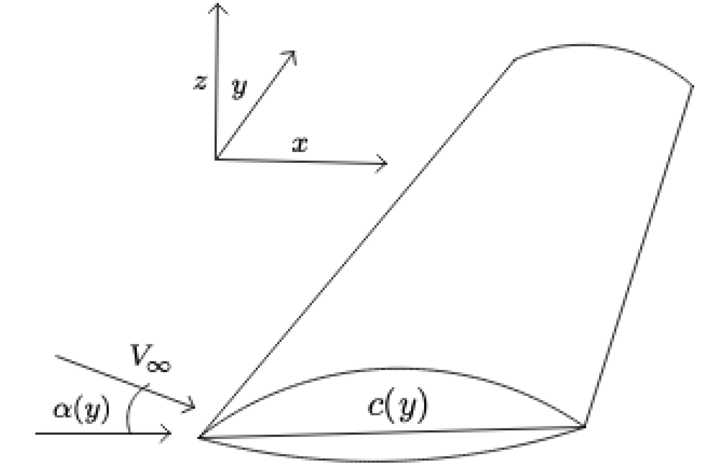
2.1. Terminology

Let x be a point in the three-dimensional space with the coordinates (x,y,z), and the fluid velocity u in terms of time t and space point x is denoted as u(x,t) = (u,v,w). The critical Mach number for a low speed aircraft is 0.3, and when Ma < 0.3, the compression effect is neglected and is treated as incompressible flow. The cruise speed of an agricultural spraying monoplane is typically less than 100 m/s, and it belongs to a category of low-speed aircrafts.

The curl of the velocity is also known as the vorticity. If the spatial distribution of the vorticity ω is known, the flow field velocity u is induced by ω and can be calculated according to the Biot–Savart law:

$$\mathbf{u}=\frac{1}{4\pi }{\displaystyle {\int }_{\mathsf{\Omega }}\frac{\mathsf{\omega }({\mathbf{x}}^{\prime },t)\times (\mathbf{x}-{\mathbf{x}}^{\prime })}{|\mathbf{x}-{\mathbf{x}}^{\prime }|}}d{\mathbf{x}}^{\prime }$$

(1)

Define the Cartesian coordinate system and airfoil section as sketched in Figure 1. Let b, s = b/2 be the wingspan and semispan respectively, and c(y) be the chord line at point y along the wingspan direction. The freestream velocity is denoted by V_∞ equivalent to flight speed; the included angle between freestream and the chord line c(y) is the angle of attack α(y).

2.2. Induced Velocity Field

2.2.1. Lifting Line Model

The classical lifting line theory can predict lift or loading distribution over a wing based on its geometry [12]. The whole finite wing is attached with ideal bound vortices, which shed as free vortices from the trailing edge, extending to infinity and forming horseshoe vortices. In this model, a large number of horseshoe vortices are superimposed tightly on the wing, each with a different length of bound vortex. All the bound vortices overlap along a single line, called the lifting line. With this theory the velocity field around wing can be calculated.

Let α_{L = 0} be the airfoil angle of attack when lift L is 0 and Γ(y) be the circulation developed over the airfoil at cross section y. According to the lifting line model, there is the following equation [12]:

$$\alpha (y)=\frac{\mathsf{\Gamma }(y)}{\pi V_{\infty }c(y)}+{\alpha }_{L=0}(y)+\frac{1}{4\pi V_{\infty }}{\displaystyle {\int }_{-\frac{b}{2}}^{\frac{b}{2}}\frac{d\mathsf{\Gamma }(\eta )}{y-\eta }}$$

(2)

where α, c, V_∞, α_{L = 0} are all known parameters about airfoil geometry and flight conditions. The function in (2) to be solved is the airfoil circulation distribution Γ(y). The above equation is a singular integral equation and has been very well investigated in mathematical theory and numerical analysis [24].

According to the Formula (1), the downwash velocity w induced by the circulation Γ at a point y over the wingspan is:

$$w(y)=-\frac{1}{4\pi }{\displaystyle {\int }_{-\frac{b}{2}}^{\frac{b}{2}}\frac{d\mathsf{\Gamma }(\eta )}{y-\eta }}$$

(3)

Different from the general purpose of aerodynamic analysis and design in the traditional aeronautical field, the entire induced velocity field, rather than the downwash over the wing only, is expected to be known in aerial spraying drift prediction.

Now consider a horseshoe vortex of infinitesimal span ds (circulation Γ) on the wing with trailing vortex filaments I, J, as shown in Figure 2. Take any point A(x,y,z) in the space around the wing, then the velocity at this point is composition of velocity induced by the bound vortex ds and vortex filaments I, J. Let OB = n, OA = r, other geometric symbols and labels see Figure 2. Points B, N, M stand for the projections of point A on the plane x = 0, the plane y = 0 and the z-axis, respectively. From the analysis of Milne-Thomson [25], the induced velocity u = (u,v,w) at point A is:

$$\{\begin{array}{l}u={\displaystyle {\int }_{-\frac{b}{2}}^{\frac{b}{2}}\frac{d\mathsf{\Gamma }}{4\pi r^2}}\cos \theta \cos \varphi \\ v={\displaystyle {\int }_{-\frac{b}{2}}^{\frac{b}{2}}\frac{d\mathsf{\Gamma }}{4\pi }}\sin 2\varphi \left(\frac{1+\sin \theta }{n^2}+\frac{\sin \theta }{2r^2}\right)\\ w={\displaystyle {\int }_{-\frac{b}{2}}^{\frac{b}{2}}\frac{d\mathsf{\Gamma }}{4\pi }}\left(\frac{(1+\sin \theta )\cos 2\varphi }{n^2}+\frac{\sin \theta (1+\cos 2\varphi )}{2r^2}\right)\end{array}$$

(4)

The basic steps of velocity field calculation are firstly solving lifting line Equation (2) to obtain the circulation distribution Γ(y), and then substituting Γ(y) into Formula (4) to achieve the velocity u for each point in space. Equation (2) and Formula (4) generally do not have an analytical solution, but their numerical solutions can be completed in a very short time, typically 2.1 s on a common PC (CPU 2 GHz, memory 2 GB). The related parameters in the Equation (2) have been determined by the wing structure and airfoil geometry, with the exception of flight speed V_∞ to which the circulation is linearly proportional. Therefore, the shape of circulation Γ(y) is directly related to the aircraft structure itself and can be acquired entirely in advance. In fact, most agricultural fixed-wing aircraft have three types of lift distribution [8], namely rectangular, elliptical, and triangular, without the need to solve Equation (2).

The two velocity components u and v are small, and the velocity field is dominated by the vertical z component, the downwash velocity w. For special spatial locations and lift distribution, the induced velocity Formula (4) can be further simplified to improve the speed of computing. For the spatial position (x,y,z), just below the wing where nozzles are mounted, in Figure 2 the point A is identical to the point B. And the downwash velocity w is given by:

$$w={\displaystyle {\int }_0^{b/2}\frac{d\mathsf{\Gamma }(\xi )}{4\pi }}\left(\frac{y+\xi }{{(y+\xi )}^2+z^2}-\frac{y-\xi }{{(y-\xi )}^2+z^2}\right)$$

(5)

2.2.2. Wingtip Vortices Model

The lifting line model is an idealization of the vortex sheet shed at the trailing edge of the wing, but this trailed vortex sheet is unstable, and the self-induced velocities make the sheet roll up and develop fully into wingtip vortices within several seconds or in the distance of a few wingspans downstream [26] (referred to as the far-field this paper) where the vorticity concentrates and constructs a counter-rotating vortex pair left behind wing tips. In the far-field of an aircraft, the air flow field is dominated by wingtip vortices, and the velocity predicted by the lifting line Equation (2) is no longer accurate, so the induced velocity in far-field should be calculated from the wingtip vortex pair. Note that the wingtip vortices are highly concentrated and can be equated to point vortices. The induced velocity formula by a point vortex can be thus employed and can calculate the velocity efficiently in far-field.

It is known that the wing circulation can be expressed in terms of the gross weight W and freestream speed V_∞:

$$\mathsf{\Gamma }=\frac{W}{{\rho }_{\infty }{V}_{\infty }b}$$

(6)

where ρ_∞ is the atmospheric density. From Formula (1) it can be deduced that the tangential induced velocity by a point vortex is:

$$v=\frac{\mathsf{\Gamma }}{2\pi r}$$

r is the radial distance of a given point to the vortex center.

To be precise, the NASA Burnham–Hallock model correlating well with experimental data is adopted, and the tangential velocity is then given by:

$$v=\frac{\mathsf{\Gamma }}{2\pi r}\frac{r^2}{r^2+r_c^2}$$

r_c is the vortex core radius defined at which the velocity v is a maximum. This vortex core radius is in general selected to be r_c = 0.052b₀, b₀ is the vortex separation [27].

It is clear that the induced velocity is proportional to the aircraft gross weight or the circulation, and inversely proportional to the distance. The trailing edge sheds many pairs of wingtip vortices behind it over time, the scope of which is two-dimensional. For any point P(x₀,y,z) corresponding to the downstream distance x₀ on a plane at which a point vortex pair locates, the velocity is contributed by this certain vortex pair. The velocity is:

$$v=\frac{\mathsf{\Gamma }}{2\pi }(\frac{1}{r_1}+\frac{1}{r_2})$$

(7)

where r₁ and r₂ are the distances between point P and two wingtip vortices, respectively. When the downstream distance x₀ varies, the value of circulation Γ changes with it because of atmospheric viscosity. Defining the initial circulation Γ₀, the circulation in terms of decay time t and radial distance r is:

$$\mathsf{\Gamma }={\mathsf{\Gamma }}_0(1-e^{-r^2/4\mu t})$$

The dynamic viscosity of air μ is of the order of 10⁻⁵ kg/(m·s) in the aerial application environment. Then it is found that the changing of Γ becomes apparent only after the time t is approaching 10⁴~10⁵ s, well beyond the far-field investigated in this paper. Therefore, on addressing wake vortices decay, the atmospheric turbulence is here primarily considered just ignoring the effect of air viscosity. Set q root mean square (rms) of turbulent velocity, and it has [28]:

$$\mathsf{\Gamma }={\mathsf{\Gamma }}_0{e}^{-0.82qt/b}={\mathsf{\Gamma }}_0{e}^{-0.82q{x}_0/V_{\infty }b}$$

(8)

Then the far-field velocity calculation procedure is as follows for any point P(x₀,y,z): 1. calculate the initial circulation according to Equation (6); 2. calculate the circulation at the distance of downstream x₀ from Formula (8); 3. determine the distances r₁ and r₂ and compute the induced velocity at point P through Formula (7); 4. decompose the tangential velocity into components of y and z direction. It should be noted that the wingtip vortices are also in motion by their self-induced velocity. The problem of position of vortex pair is to be dealt with later.

2.2.3. Mixture Model

There are several prerequisites for the application of classical lifting line theory [12]: 1. the aircraft has a high aspect ratio, AR > 4; 2. the aircraft is of a thin airfoil type, non-swept or delta wing; 3. low flight speed, that is, Mach number Ma < 0.3; 4. the trailed vortex filaments are parallel to the direction of flight motion, under which the interactions between the vortex filaments are ignored. For almost all agricultural fixed-wing monoplanes, the first three conditions are satisfied. Due to their repulsive nature, the mutual induction between vortex filaments makes the trailed vortex sheet move outward and roll up, finally forming regions of concentrated vorticity moving downward. Generally, the wingtip vortices are regarded to be fully developed within a time t₀ = b²/2Γ₀ [13]. Beyond a distance corresponding to the moment t₀, it is treated as far-field where the wingtip vortices model works, otherwise it is near-field in which is the sphere of application of the lifting line model. Therefore, the lifting line-wingtip vortices mixture model is established to just match two evolving phases of trailing vortices and bypass the assumption of the parallel vortex sheet.

2.2.4. Trajectory Approximation

The particle trajectory in velocity field is under the action of forces that are mainly the gravity and the aerodynamic drag. It can be modeled by Newton’s second law within the Lagrangian framework. The particle trajectory (y, z) in the flow filed subjects to the general equation [8]:

$$\{\begin{array}{l}{y}^{″}=(v-y^{\prime })/{\tau }_p\\ z^{″}=(w-z^{\prime })/{\tau }_p-g\end{array}$$

(9)

where (v, w) is the induced velocity in the flow field, τ_p is the particle relaxation time, g the standard acceleration due to gravity. The relaxation time τ_p is computed from:

$${\tau }_p=\frac{4}{3}\frac{D_p{\rho }_p}{C_D{\rho }_{\infty }{V}_{rel}}$$

(10)

and ρ_∞, ρ_p is the density of air and the particle. respectively, D_p the particle diameter, V_rel the relative velocity to the flow field. The drag coefficient C_D is given by [29]:

$$C_D=\frac{24}{\mathrm{Re}}{(1+0.27\mathrm{Re})}^{0.43}+0.47[1-\exp (-0.04{\mathrm{Re}}^{0.38})]$$

(11)

For 2 × 10⁻³ < Re < 2 × 10⁵, the Reynolds number of a particle Re is defined as:

$$\mathrm{Re}=\frac{V_{rel}{D}_p}{\nu }$$

(12)

where ν is the kinematic viscosity of air.

The relaxation time τ_p and related aerodynamic drag are often nonlinear in terms of the relative velocity due to the particle size spread out across a wide range. It will make trajectory of tacking for an ensemble of particles computationally intensive. In order to achieve a simplified analysis, only three kinds of particles, namely very coarse, median, and very fine, are dealt with. Especially for very fine particles (smaller than 20 μm), it has a sufficiently small Reynolds number to be in the Stokes flow regime, and Equation (9) reduces to a linear form as relaxation time becomes:

$${\tau }_p=\frac{D_p^2{\rho }_p}{36\nu {\rho }_{\infty }}$$

In this instance, the path lines of velocity field will be good approximations to particle trajectories.

The released particles from a nozzle disperse over the ground, satisfying some probability distribution, other than deposit on a certain spot due to turbulent diffusion and their wide spectrum of size. This probability distribution of ground depositions is usually considered to be normal to consider the effect of random fluctuation as a whole consisting of the turbulence of airflow. Then the Gaussian mixture model is applied to predict deposition concerning the dispersal of particles from several nozzles mounted at different positions. More specifically, suppose there are N number of nozzles onboard with the same flow rate and the fraction of ground deposition from all released particles is in terms of a coordinate variable y, denoted as G(y) on y-axis. This fraction contributed by nozzles equally is the sum of particle portions from individual nozzles called subpopulations in a statistical term [30]. Each subpopulation is subjected to the Gaussian distribution with mean μ_i and standard deviation σ_i (i = 1,…, N). Then the overall population, namely the total fraction, meets with the Gaussian mixture model expressed as:

$$G(y)=\frac{1}{N}{\displaystyle \sum _{i=1}^N\frac{1}{{\sigma }_i\sqrt{2\pi }}\exp \left(-\frac{{(y-{\mu }_i)}^2}{2{\sigma }_i^2}\right)}$$

where the mean μ_i and standard deviation σ_i (i = 1,…, N) is determined by positions of ground deposits of three typical particles mentioned in the above. Finally, the particle deposition spreading over the ground is resolved through the Lagrangian dynamics on considering certainty contained and the Gaussian mixture model dealing with stochasticity corresponding to the turbulent effect of the airflow and other factors not included in the deterministic strategy, such as particles with sizes out of our formulas.

2.3. Wake Vortices Motion

In addition to induced velocity field, the motion of released droplets is also affected by wake vortices. The wake evolves from the boundary layer that is the part of the flow in the immediate vicinity of an aircraft where the effect of viscosity is significant and vorticity eventually turns into wingtip vortices trailing downstream at a velocity nearly as the freestream. Wingtip vortices’ behavior, decay, and transport can redistribute the induced velocity field to make it unsteady and influence spraying droplet trails. The present study focuses on fast time modeling of wingtip vortices evolution with the ground proximity, also combined with crosswind, by the point vortex dynamics method, which was introduced and has been the issue of extensive investigation in air traffic control [31,32,33].

The initial wingtip vortices system is composed of two counter-rotating vortices, called primary vortices, laterally separated by a distance b₀. The primary vortices firstly sink due to their interference at a constant velocity out-of-ground effect (OGE). As they approach the ground, ground effect takes place and leads to lateral separation of them where it is labeled as the near-ground effect (NGE) region. The vortices then go further down and begin to interact strongly with the ground, entering the region of in-ground effect (IGE). The boundary layer close to ground is produced, detached, and two secondary vortices with opposite sign vorticity are generated beneath each primary vortex. The interaction of primary and secondary vortices leads the vortex rebound, rising again to a new height. Subsequently, the vortex system even induces more secondary vortices if given enough circulation, disperses, and finally is fading away in the atmosphere.

The evolution process of wingtip vortices can be divided into three phases, as described in Figure 3.

• In the OGE phase (Figure 3a), it is a two-vortex system, circulation decay subjecting to Formula (8), and the downward velocity is Γ/2πb₀.
• In the NGE phase, at a height of h₁ = b₀*ZIMFAC above the ground, it is a four-vortex system (Figure 3b). Two image vortices are added below the ground as the mirror of primary vortices to meet the boundary condition of zero vertical velocity at the ground. Because of the symmetry, the trajectory of only starboard vortex is addressed. Here ZIMFAC stands for “z image factor” determined by experience. It has:

  $$\{\begin{array}{l}\frac{dy}{dt}=\frac{\mathsf{\Gamma }}{4\pi }(\frac{1}{z}-\frac{z}{y^2+z^2})\hfill \\ \frac{dz}{dt}=-\frac{\mathsf{\Gamma }}{4\pi }(\frac{1}{y}-\frac{y}{y^2+z^2})\hfill \end{array}$$

  (13)

  where (y,z) is the starboard vortex position. If the flow is inviscid, it was demonstrated by Saffman [34] that this NGE phase will be the end, the secondary vorticity cannot be generated, hence the primary vortices descend and move outward reaching to the asymptotic altitude d₀/2 expressed by:

  $$\frac{d_0}{2}=\frac{b_0}{\sqrt{{(b_0/h_0)}^2+4}}$$

  (14)

  where h₀ is the initial altitude that a primary vortex pair generates.
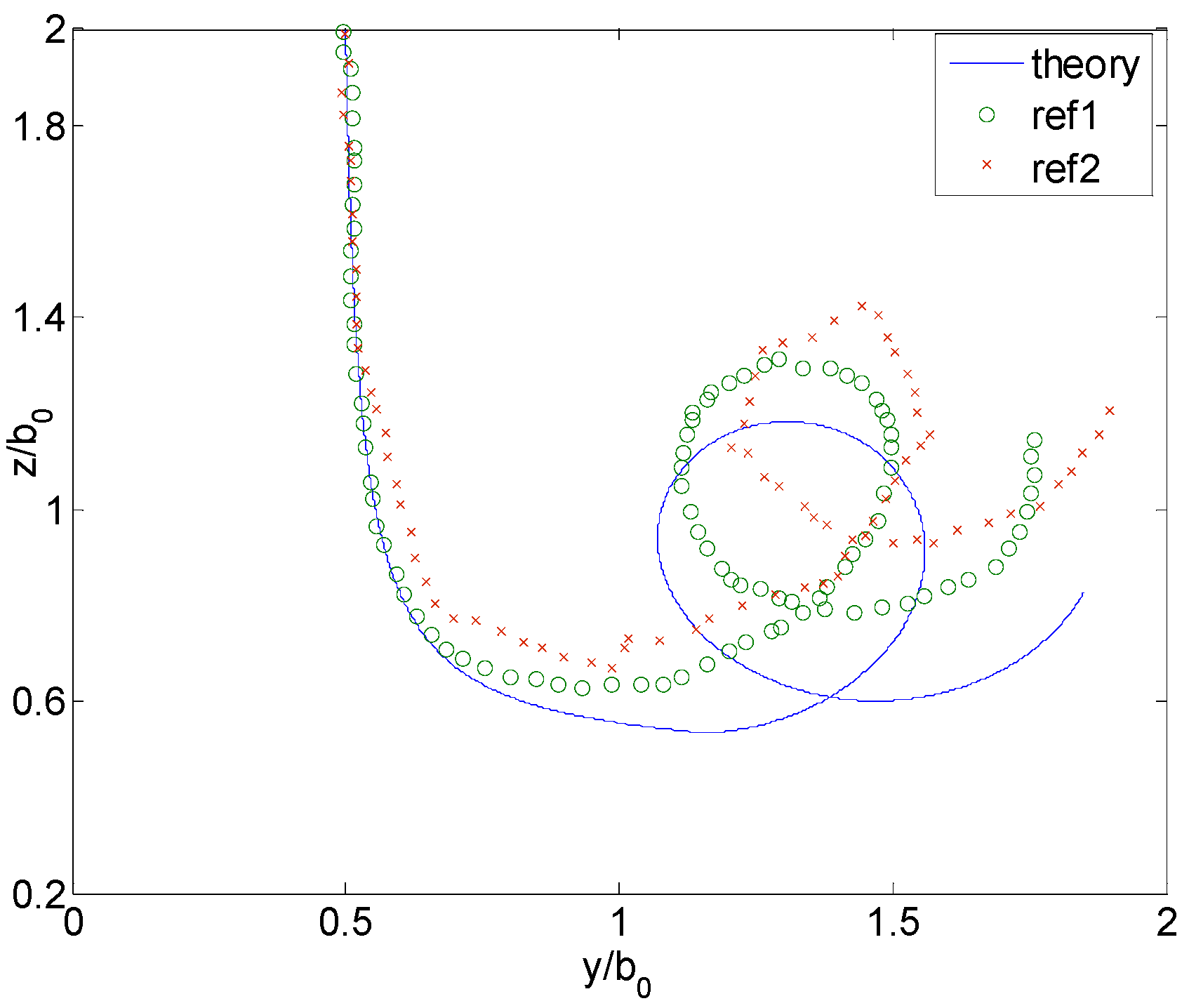
• In the IGE phase, at a height of h₂ = b₀*ZGEFAC (for “z ground effect factor”) above the ground, it is an eight-vortex system (Figure 3c). The two secondary vortices and their images are introduced at a distance of b₁ and at an initial rotation angle θ of outboard of primary vortices, where θ is zero below the primary vortices and is positive clockwise for the port vortex or counterclockwise for the starboard vortex [33]. The initial ratio between secondary and primary circulation is defined as γ. Set (y_i,z_i) (i = 1,…,8) the position of vortices, this eight-vortex system is subjected to the following Equation (15) of point vortex dynamics:

  $$\{\begin{array}{l}\frac{d{y}_i}{dt}=-\frac{1}{2\pi }{\displaystyle \sum _{i\ne j}{\mathsf{\Gamma }}_j}\left(z_j-z_i\right)/r_{ij}^2\hfill \\ \frac{d{z}_i}{dt}=\frac{1}{2\pi }{\displaystyle \sum _{i\ne j}{\mathsf{\Gamma }}_j}\left(y_j-y_i\right)/r_{ij}^2\hfill \end{array}$$

  (15)

  of which $r_{ij}^2={\left(x_j-x_i\right)}^2+{\left(y_j-y_i\right)}^2$.

Now take the effect of crosswind into consideration. The velocity profile is usually represented in terms of the altitude according to the atmospheric boundary layer theory but neglecting stratification effect [35]. In near neutral conditions, the logarithmic law of the wind profile above the plant canopies reads:

$$v(z)=\frac{u_{*}}{\kappa }\ln (\frac{z-d}{z_0})$$

where u_* is the friction velocity, κ = 0.4 is the von Karman constant, d the displacement height typically equals to 75% of the canopy height h_c, z₀ = h_c/30 indicated by laboratory measurements is the roughness length. The crosswind affects the lateral drift in the spanwise direction. The crosswind term will be added to right side of the ODEs (15) with respected to dy/dt.

3. Results and Analysis

3.1. Induced Velocity Distribution

Take the aircraft body coordinate frame as Figure 1. Suppose the elliptic and rectangular lift distribution respectively over the wing, then the vertical velocity on the yz plane at x = 0 and its section lines where nozzles locate exactly below the wing is shown in Figure 4. The z-direction velocity w is divided by the factor W₀ to be dimensionless, in which W₀ = Γ₀/2πb. As seen from Figure 4a,b the induced velocity is symmetric about the z-axis. The velocity appears negative (downwash flow) within the wingspan, but becomes positive (upwash flow) beyond it and decays to be zero. Combined with Figure 4c,d the induced maximal downward velocity corresponding to the elliptic lift is at y = 0, z ≈ −0.1b, the wing root region, while the maximal downwash of rectangular lift approaches the wingtips.

For both elliptic and rectangular lift distribution, the downwash flow region becomes narrower but its value is greater when it draws closer to the wing, because the distance between this region and the vortex core gets shorter. From the intersection points in Figure 4c,d, one can resolve locations of vortex cores are at y = ±0.43b (elliptic lift) and y = ±0.5b (rectangular lift), where the precise location measured in [8] is y = ±0.39b and y = ±0.5b for elliptic and rectangular lift, respectively. Meanwhile, it is found that the rectangular lift generally tends to induce greater velocity than the elliptic distribution given the same factor W₀. Therefore, an agricultural aircraft with rectangular lift is preferred in aerial spraying and the nozzles should be mounted within the downwash flow region.

In the far-filed the downwash flow field on the yz plane is calculated according to Equations (7) and (8) with q = 0.7m/s, x/b = 2 (two wingspans downstream). It is shown in Figure 5a that the pattern of induced velocity on section lines z = −0.1b, −0.3b, −0.5b is nearly consistent with that in Figure 4d, but different from the velocity distribution in Figure 4c. This indicates that the lifting line model can be replaced by the wingtip vortices for rectangular lift to achieve a faster performance. The velocity field in Figure 5b suggests the released particles near wingtips (y/b = ±0.5) may move outward and upward, to cause a potential dispersion.

Now we compare the downwash velocity profile from mixture model to CFD result and field measurement of [14] in the near- and far-field. For the fixed-wing aircraft Thrush 510G there are related parameters described in

Table 1. The parameters of Thrush 510G aerial spraying.

Parameter	Gross Weight	Wingspan	Flight Altitude	Release Height	Flight Speed	Air Density	Wind
Value	4367 kg	14.47 m	5 m	4.7 m	55 m/s	1.29 kg/m3	4 m/s

, in which the release height and flight altitude take the ground as the reference plane. In the following, the Thrush 510G aircraft and its spraying parameters will be repeatedly applied unless otherwise stated. The initial circulation of wing is obtained from Formula (6) Γ₀ = 61 m²/s. To agree with the setting in [14] the center of velocity curve is set at y = 6 m, and the comparison of velocity distribution under the wing above the ground 3 m corresponding to z = −0.14b is shown in Figure 6. The crosswind blows the starboard vortex slightly higher than the port vortex, so the velocity profile is asymmetric and the downwash value near the starboard vortex is smaller compared to the port vortex, which was also demonstrated in [31]. But to our surprise, the maximal vertical velocity error is less than 0.5 m/s even out of consideration the effect of crosswind in our model.

The far-field induced velocity of Thrush 510G is calculated using the wingtip vortices model. Get the position in the downstream x/b = 7.6, 38, 76, 190 corresponding to the time t = 2 s, 10 s, 20 s, 50 s. The velocity and error distributed on the section line along y-axis over the ground h = 3 m are shown in Figure 7. The induced velocity is not more than 2 m/s and gradually decays to zero with the elapsing of time because the circulation of vortices dissipates in the atmosphere and its effect becomes negligible. The average errors on the y-axis, E_dav, E_uav of both downwash and upwash read less than 0.5 m/s within 50 s from Figure 7b, and the maximal velocity errors, E_d, E_u, are less than 1.5 m/s at t = 2 s, then reach the peak (less than 1.7 m/s) appearing at t = 10 s the moment vortex rebound and secondary vortices begin to happen. Simultaneously, the maximal and average relative errors also have the largest values at t = 2 s and subsequently decay as seen in Figure 7c. Although this vortex evolution mechanism has not been considered, it is found that it does affect the downwash flow field very slightly, especially in the late stage of wake evolution. In any case, from the aspect of relative errors the lifting line-wingtip vortices mixture model does not work very well as the average relative error of downwash is nearly 18% and average relative error of upwash is about 10% in the whole course of wingtip vortices life cycle. But note it is the absolute error, other than relative error, that imposes negative effects on the accuracy of analysis more so this model has a satisfactory performance for rapid velocity calculation though relative erros are large.

3.2. Vortex Trajectory

Let the origin of z-axis be on the ground. Initially wake vortices generating at the point (Y₀, Z₀) = (5.65, 5) for Thrush 510G, are already in the NGE phase indicated by Figure 3b because the vortex separation b₀ = 2Y₀, the height Z₀ < h₁= b₀*ZIMFAC where ZIMFAC = 1.5 [33]. The image vortex allows the primary vortex to acquire an outward velocity component, while in the OGE phase the primary vortices of a two-vortex system can only have a downward velocity just induced from the other primary vortex behaving like a free fall. In different phases the patterns of starboard vortex are described in Figure 8. The NGE phase is dominated by the outward velocity significantly greater than the downward component, and then the primary vortex will approach to the certain height d₀/2 = 3.74 m computed from Formula (14) but not impacting the ground. This behavior is unfavorable in aerial spraying.

In the aircraft vortex spacing research [33] the characteristic height of IGE phase is assumed to be h₂ = 0.6b₀. Sometimes the initial height of primary vortices Z₀ is already within the range. But the vortex system does not fall into IGE phase immediately. The secondary vortices generation is an indication that the IGE phase needs time to evolve. The vortex system have to firstly experience NGE phase, and then transfers to the IGE phase in several seconds. This time duration depends essentially on primary vortices’ release height, initial circulation and their decaying rate. If the vortex evolving starts from the OGE phase, the full stages can be observed that it begins to descend in OGE phase, and then move outward in NGE phase, afterward the altitude approaching 0.6b₀ it enters IGE phase. Vortex rebound is a typical phenomenon in extreme ground effect depicted in Figure 9. The secondary vortex, which has the opposite sign of circulation, gives the primary vortex a velocity upward. Under different conditions the primary vortex in IGE phase is to be in U turn motion just moving up, or loop itself as shown in Figure 9. The accurate trajectory of vortex motion is related to the setting of relevant parameters. To agree with results described in Figure 9, characteristic parameters in IGE phase are given by

Table 2. Description, symbols, and values of the parameters in the IGE phase. The suggested values are based on the papers [32,33] and the comparison of theoretic results with those of [14,15].

Description	Distance between Primary and Secondary Vortex	Initial Rotation Angle from Primary Vortex	Initial Ratio between Secondary and Primary Circulation	z Ground Effect Factor
Symbol	b1	θ	γ	ZGEFAC
Value	0.17b0	π/10	0.64	0.6

. But in presence of crosswind, it is believed that the crosswind shear makes a redistribution of the vorticity that contained in the boundary layer, and the high crosswind suppresses the creation of secondary vortex, leading to the weakness of vortex rebound.

3.3. Validation of Fast Analysis

In this subsection, the spray trails and drift or dispersion are estimated by fast analysis method and are compared to results of CFD simulation [19], AGDISP and field experiment. Thrush 510G is again taken as the spraying aircraft. Ten nozzles of a spray line are mounted under the wing at y = ±5 m, ±4 m, ±3 m, ±2 m, ±1 m. The rotary cage atomizer is adopted to assume a zero outlet velocity. The diameter range and mass fraction of droplet size distribution is presented in Figure 10. Other input parameters follow Table 1 or are referred to [19].

3.3.1. No Wind

In the absence of wind, at first only the NGE phase is considered in the model. To implement our fast analysis method, the motion of two kinds of sizes, the coarsest and finest droplets, are analyzed. The coarsest droplets (670 μm) are very heavy compared to air, supposed to be free-falling down, then their positions have no spanwise displacement as same as the initialization. And the trajectories of finest droplets (10 μm) are treated as path lines of velocity field because they are small enough to be in the Stokes flow regime moving with the local velocity. Figure 11 gives trajectories of fine droplets. Only six trails deposit on the ground, that is, intersecting the line z = 0. The droplets releasing from other four nozzles near the wingtips are drawn into wake vortices, their corresponding trails revolving in the air not easy down to the ground. The y-axis coordinates of depositing points of 10 μm and 670 μm droplets then give the boundaries y_m, y_M of deposition on the ground, between which other droplets own the high probability of falling. Considering droplet size distribution (Figure 10), the deposition pattern of spray particles is expressed as ideal stem plots in Figure 12. There are six stems appearing in this figure corresponding to nozzles from which droplets deposit on the ground while others disperse beyond the region. Note that the 177 μm droplets occupy the largest fraction in the volume; they are represented as peaks in the figure. It is evident that the deposition of fine droplet is close to the position of 10 μm droplet, and the coarse droplet near that of 670 μm droplet.

However, the real ground deposition cannot be that as in Figure 12 so regularly, due to atmosphere turbulence and other random variations. From each nozzle droplets disperse along y-axis out of the range limited by the coarsest and the finest particles, obeying a probability distribution assumed to be Gaussian generally. Take y-value related to the peak as the mean μ, the difference |y_M − y_m| as the variance σ, then there is a Gaussian mixture model containing six normal distributions also shown in Figure 12. Adding these Gaussian distributions obtains the deposition curve of NGE phase from all nozzles in a spray line described in Figure 13. The droplets from two nozzles at y = ±1 m are found to be highly concentrated having the maximal deposition, since the outward velocity in the central region is small and favorable to deposition. But compared to the prediction by CFD the deposition curve is too narrow, revealing the dispersal effect of NGE phase in the spanwise direction has not been adequately accounted for.

In the IGE model, the primary and secondary vortices both rebound aloft and extend to the distance spanwisely reducing the downward velocity in flow field and giving particles outward velocity near the ground. For symmetry only the starboard vortices trajectories are shown in Figure 14. Hence the droplets will disperse farther than in the NGE model because of the induction effect of secondary vortices. The trajectories of droplets with three typical sizes are presented in Figure 15. It is noticed that all the path lines and trajectories of 10 μm droplet do not intersect with the ground z = 0 (Figure 15a,b). In practice they may need more time to transport in the air and randomly impact the ground through turbulent diffusion. In the vortex core region, fine droplets including 137 μm are easily rolled into it, and are distributed evenly to move with it (Figure 15c). In the middle of the velocity field there is a lateral air flow, smaller droplets having short relaxation times, and they tend to follow the flow. But larger droplets, for example, with the size 137 μm, can escape. The very coarse droplets (670 μm) that the gravity dominates can also be affected by the wake vortices being dragged to the vortex region, although they drive through the vortex core and deposit onto the ground (Figure 15d). In aerial spraying, the wake vortices and their induced outward velocity impose a negative effect on the droplet deposition. The finer the droplets are, the more easily they are subjected to the airflow. By our theoretical computation it is observed that droplets from the middle four nozzles can deposit on the ground increasing the size to 120 μm, the middle six can escape from vortices with 180 μm, and only when the size is 280 μm can all the droplets start to settle on the ground. Therefore, the entrainment of droplets need not take place in the vortex core region. Provided the droplets are small enough, or close to the vortex, they will be in the action scope of vortices and be trapped by the flow field suspending in the air, though nozzles are placed out of the vortex radius.

The Gaussian mixture model is also applied in the IGE phase. But this time, the ground deposition positions of droplets of VMD 137 μm are taken as the means of Gaussian distributions. The variances are the distance from deposition positions of 137 μm droplets to those corresponding coordinates of 670 μm. The deposition curve of IGE phase is hence obtained and is also shown in Figure 13. The profile, minimal, and maximal deposition positions of the IGE model, better than NGE model, agree well with those of CFD simulation. The droplets dispersal region in CFD is wider than NGE and IGE, and the deposition fraction of pesticide applied predicted by CFD is also much more than two models. The reason is that the droplets deposition from nozzles in the outmost is not considered in the Gaussian mixture model, since by theoretic computation they are not deposited on the ground.

3.3.2. Effect of Crosswind

The crosswind only by itself does not have such a great effect upon the droplets drift that make it travel to a long distance up to 20 km [6]. Instead, it distorts the movement of wake vortices that they are in absence of wind, and hence redistributes the induced velocity field. Take the friction velocity u_* = 0.13 m/s regarding the 2 m/s crosswind at the height of 4 m over the ground, and the vertical wind speed is subjected to the logarithmic law, while the headwind is assumed to be zero. The IGE phase is considered. Trajectories of wake vortices affected by the crosswind are presented in Figure 16. Because of the wind, the symmetry of vortex trajectories is broken. The primary and secondary vortices rebound is suppressed by the crosswind and is somewhat lower than in Figure 14. For persisting at least 50 s they float in the air and hardly deposit onto the ground. The trails of fine droplets will be seriously influenced by the suspending of wake vortices.

The droplet trajectories of three typical sizes are exhibited in Figure 17, Figure 18 and Figure 19. Figure 17a,c is 10 μm droplet trajectories dispersing along y-axis (spanwise direction) are calculated from Lagrangian method, the Equation (9) and AGDISP, respectively. The dispersion along x-axis (flight line direction) can be seen in Figure 17b,d. Figure 18 and Figure 19 address trajectories of droplets with sizes of 137 μm and 670 μm, respectively. In addition, results of IGE model are compared with those of AGDISP in these figures. On dealing with behaviors of droplets near wake vortices, IGE model accounting vortex rebound is more refined than AGDISP. Both IGE model and AGDISP reveal the coarse droplets are less insensitive to drift. The fine droplets (10 μm, 137 μm) and those from nozzles near wingtips are easy to be caught by vortices (Figure 17 and Figure 18), similar to the case of no wind. But instead of in situ rotation, they transport continuously far to the downwind. Droplets close to the port vortex move higher than their counterparts in the right side, seemingly more susceptible to the crosswind. The trajectories in the right side are worked by the combined action of crosswind and the lateral velocity, which follow the same direction the velocity superposition effect taking place. Therefore, these trajectories are discovered to be inclining to the right. Deposition curves in the left side have a different movement mode. Firstly, near the releasing spots they are dominated by the wind; afterward, on approaching the ground, they are dragged by the port vortex turning to the opposite, upwind direction, as the wind speed becomes negligible. But note this is not always the case due to the complexity of vortex motion and induced unsteady velocity field. This mode more likely holds for larger droplets (Figure 18 and Figure 19).

In the aircraft flight direction, droplets start to move forward with the initial velocity, and then encounter the headwind against their motion induced by wake vortices. The coarse droplets (670 μm) have the short settling time; hence they fall on the spots ahead of the original point. The settling time of smaller droplets (10 μm, 137 μm) being long, they may only advance a little, or just move downstream which can be seen from Figure 17b,d and Figure 18b,d. Since the ground is an absorbing boundary, the traveling length of releasing particles along the x-axis is determined by the time required to cover the distance in the vertical direction. Because induced x-component velocity is small according to Formula (4) it thus appears to be a contradiction of AGDISP results that all droplets deposit onto the ground not too far behind Thrush 510G in Figure 18d, but on yz plane droplets from the wingtip are rolled into wake vortices aloft disclosed by Figure 18c. The particle dispersal along x-axis has not been carefully addressed so far in aerial spraying research including AGDISP. Actually, it is controlled by the flow around nozzles, which should be investigated in the future.

Based on the droplet trajectories and Gaussian mixture model, we figured out the drift or deposition curve to compare with CFD [19] and AGDISP in Figure 20. The curve is asymmetrical with a long tail in the right side caused by wind. As our theoretic result does not consider the settling of droplets within the working region of wake vortices, the downwind dispersion distance is about 150 m, less than the estimation by CFD and AGDISP that is nearly 300 m. Therefore, it is also restrictive on estimating deposition fraction of pesticide applied. But the theoretical model successfully predicts the furthest drift position in upwind direction, about −20 m, nearly as the same as estimated by CFD and AGDISP. Around the original point there are several peaks reported by all three methods. The peak positions in our theory concerning ground deposition of 137 μm droplets only have slight differences from those of the other two curves. At the expense of accuracy in some degrees, our theoretic model runs very quickly and completes within 3.2 s on a common PC (CPU 2 GHz, memory 2 GB). In contrast, AGDISP takes 25 s for this case whilst CFD needs several to tens of hours.

3.3.3. Effect of Headwind

Sometimes the spray dispersion is influenced by the headwind when the aircraft flight direction is against the wind, though the crosswind is in most cases considered. In this instance, theoretically the freestream opposite to the flight direction will be accelerated by the headwind when a weaker wingtip vortex pair is produced from Formula (6), which will have less effect on droplet dispersion, and of course, at the same time the shear flow component of headwind deviating from the flight line and its local variation in a given direction could blow droplets along the spanwise direction as what the crosswind does. Our model will address the effect of headwind and compare to results of the field experiment in [2]. The spraying aircraft was Thrush 510G, flight speed 66.7 m/s, flight altitude 4 m, release height 3.7 m, deposits recovered height 0.6 m, steady northwest headwind with direction 267° (east: 0°, south: 90°, west: 180°, north: 270°), wind speed 1.3 m/s. The flight line was variably adjusted based on the wind direction ensuring angle of flight orientation, and headwind was maintained within 15°. The deposits sampler was water-sensitive paper placed along a straight line perpendicular to flight path whose sampling resolution was 3 m. Other necessary parameters are the same as the cases in the above, or are referred to [2].

Because of the low flight altitude, the IGE model is applied to handle the extreme ground effect. The results from theoretical prediction are exhibited in Figure 21. The trajectories of 137 μm droplets are asymmetry that is distorted by the crosswind component of headwind. But this crosswind effect is very little for the adaptive flight line following the headwind. After all, these two directions are not identical, resulting in the droplets dispersion along the y-axis downwind up to 25 m (Figure 21a), which is reflected in Figure 21b that ground deposition has a shift to the negative y-axis different from Figure 13. Both field measurement and our model caught this pattern, although two curves are not entirely coincidence. In addition, using water-sensitive paper to recover deposits is limited, hence in the upwind direction beyond the range of 10 m no deposits were collected in the field experiment, certainly not in line with the actual dispersion. In [2], the experiment was conducted to evaluate the effective swath width of Thrush 510G where it is determined by identifying the largest range of coverage rates that were greater than the mean. From Figure 21b the mean of deposition by IGE model is about 0.045 holding the swath from −7 m to 4.5 m, whilst the field experiment identified the interval of −6 m to 9 m. Comparing Figure 21 with Figure 18a and Figure 20, highlights the less influence of dispersion imposed by headwind rather than crosswind. Then maybe the dispersion could be restricted with flight line following the wind direction.

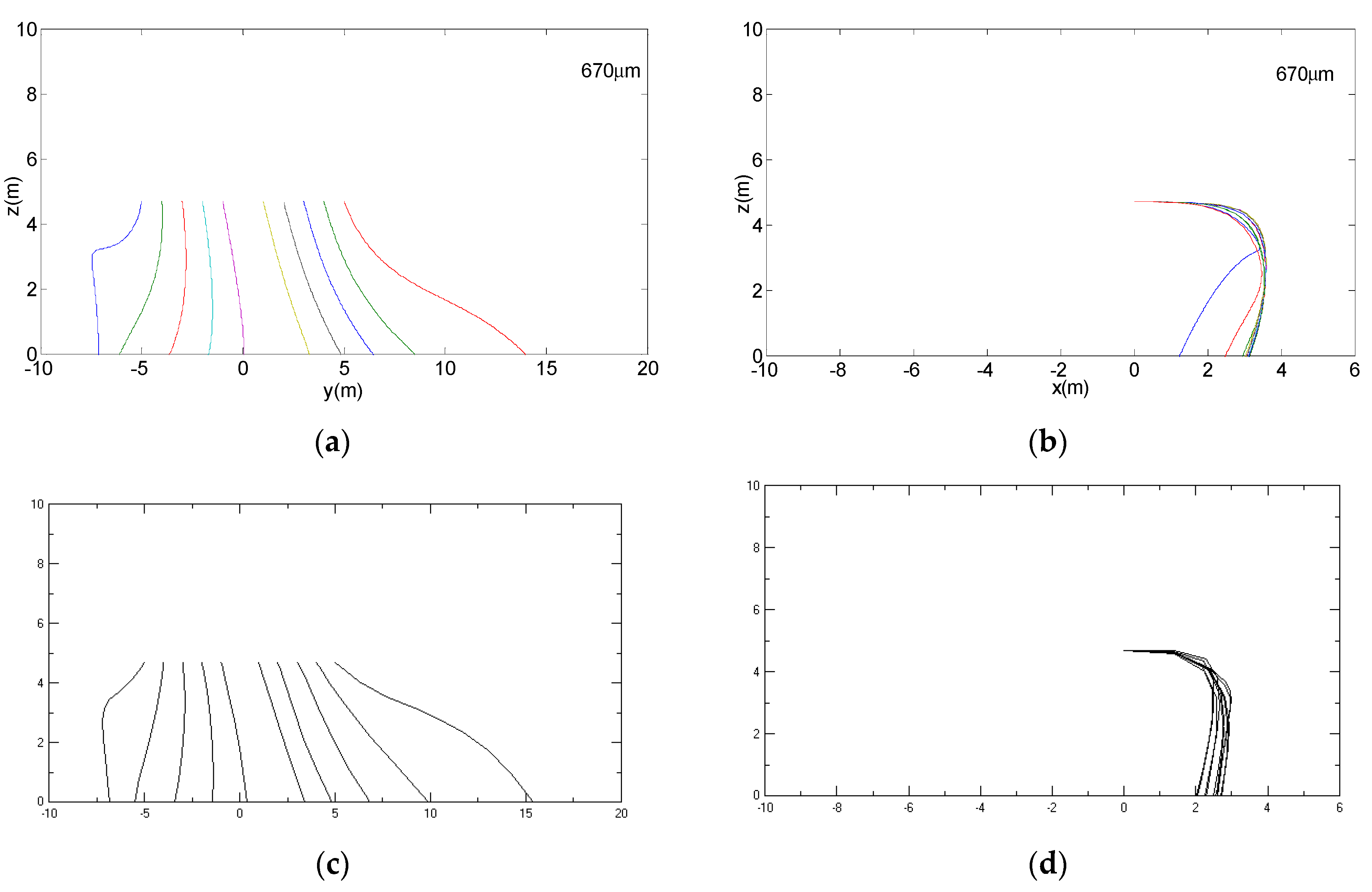
3.3.4. Relation between Droplet Size and Drift Distance

From Figure 17, Figure 18 and Figure 19 it is known that the drift distance increases when the droplet size is getting smaller. But a quantitative relation has not been established. Regarding the 1 m/s crosswind and the nozzle placement y = −5.8 m, −4.7 m, −3.65 m, −2.65 m, −1.46 m, 1.4 m, 2.58 m, 3.6 m, 4.65 m, 5.75 m, the field experiment was conducted and water-sensitive paper was used to collect the droplets [36], other parameters referring to Table 1. By comparison the average drift distance is computed from our theoretic method. The raw data and their fitting through regression analysis are shown in Figure 22. To our surprise, an approximately linear relation is obtained, that is, the drift distance linearly decreases as droplet size increases. The coefficients of determination R² for “fitting1” and “fitting2” are 0.88, 0.82, respectively, indicating a significant linear correlation of the size and drift. This relationship that is associated with the wind speed and nozzle placement yet can be used in a gross analysis. In some instances, for example, the case of Section 3.3.2 the linear relation from theoretic computation is hardly satisfied.

4. Discussion

The droplet drift or dispersal has been known to be the comprehensive result of flow field, wind speed, and factors associated with droplets, including size and spatial position. With regard to suppression of drift, the wind is just left aside since it is uncontrollable. In addition, when the spraying aircraft and flight parameters are determined, one can seldom do something to flow field. According to the results and analysis of Section 3, some solutions are thus proposed: 1. reducing proportion of fine droplets; 2. changing nozzle distribution, that is, the nozzle’s spatial position, including height and spanwise coordinate; 3. increasing droplet outlet velocity.

In the following, the solutions are investigated by our theoretical method, which was verified in the preceding section as being good as AGDISP, if not better, on predicting droplet trajectories. Intuitively, it is expected that increasing initial droplet velocity or decreasing the gap between nozzles and the ground droplets could achieve a shorter time in the air and quickly impact the ground. For coarse droplets, they are not the main contributor to the drift as seen from Figure 15d and Figure 19d. Then under what conditions and with the size to what extent the fine droplet can escape from the vortex is an issue. Setting the nozzle height z₀, droplet outlet velocity v₀, then droplet trajectories are compared in Figure 23 for their different sizes and initial states.

This suggests that the release height and initial velocity impose little effect on the dispersion of fine droplets even when their values are extended to a high extent impossible in practice, shown in Figure 23a,b and compared to Figure 15b. The best nozzle placement depends on the friction velocity that nozzle position at y = ±2 m is better than y = ±1 m without wind and y = 1 m is the best position with wind, indicated by Figure 23b–d. Therefore solution 2 and 3 cannot settle the issue of droplet drift. As disclosed by the relation in Section 3.3.4, only droplet size is the dominating factor that the drift is controllable to be within 50m with increasing the droplet size to 180 μm (Figure 23d). Then for the purpose of drift control the VMD of droplets should be large enough and the portion of fine droplets must be reduced.

5. Conclusions

This paper proposes a fast analysis to predict pesticide spray trails from an agricultural aircraft very near the ground and their drift or deposition based on calculating velocity field, resolving wake vortices motion, and tracing typical droplets, then extending to get depositions of droplets with a continuous spectrum of sizes. It has the following conclusions:

• The lifting line-wingtip vortices mixture model allows rapid calculation of the complete velocity field around an agricultural monoplane in 2.1 s on a common PC (2 GHz CPU, 2 GB RAM), and the whole fast analysis for estimating droplets trajectories and drift is implemented within 3.2 s. For the same case, AGDISP takes 25 s whilst CFD needs several to tens of hours.
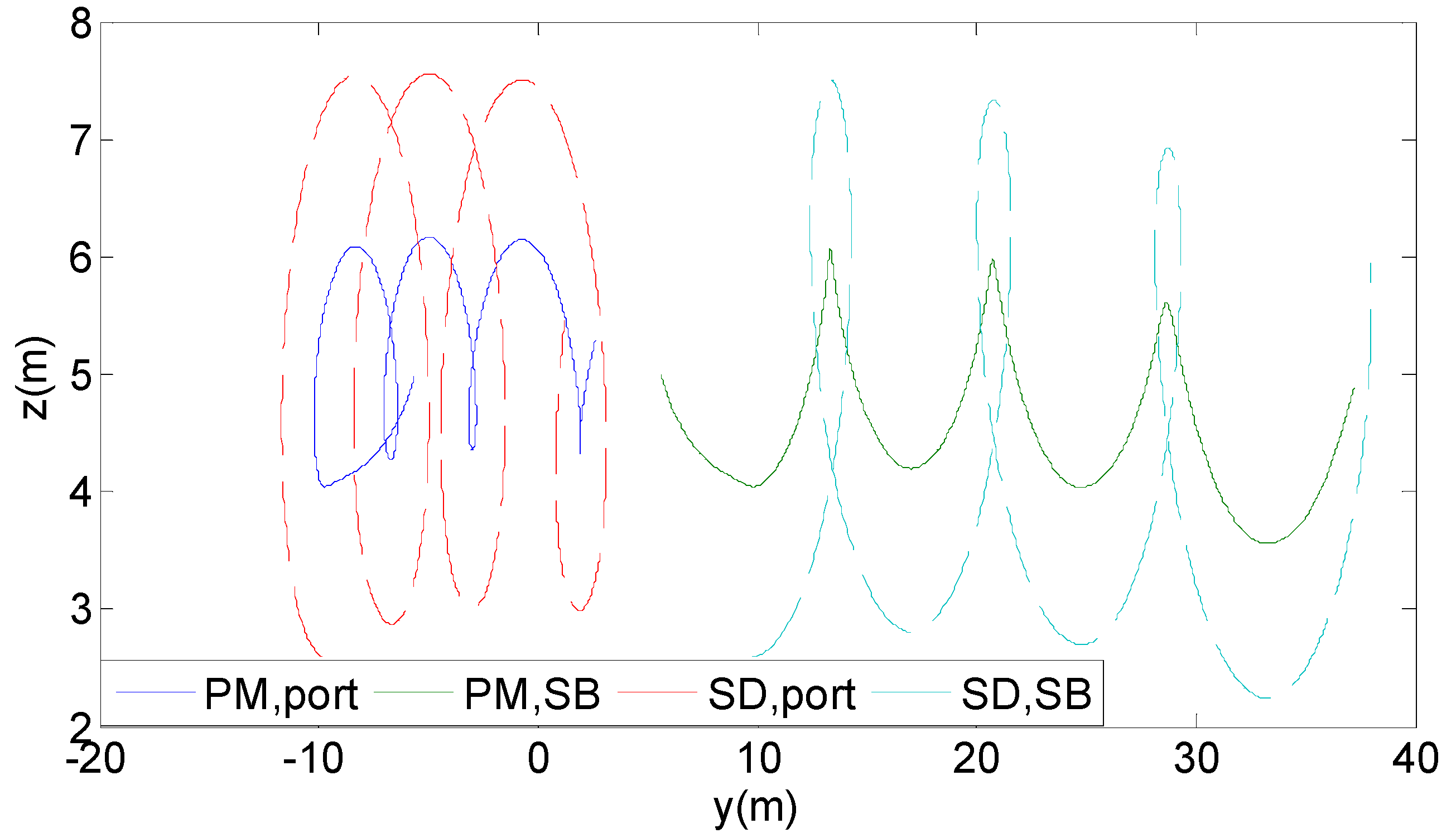
• The lifting line-wingtip vortices mixture model is in good agreement with the experimental and CFD results for Thrush 510G aircraft. At a height over the ground of 3 m, the maximum velocity error is less than 1.5 m/s and the average error is less than 0.5 m/s in the space that is 7.6 wingspans downstream of the aircraft (corresponding to a time span of 2 s). Outside this region, the maximum velocity error does not exceed 1.7 m/s, and the error tends to decrease with distance. The N-vortex system, by adding secondary vortices and their images, can predict vortex rebound and thereafter vortex motion, roughly matching with CFD simulation. The flight very near the ground could induce stronger secondary vortices, produce additional upwash flow, and result in entrainment of particles aloft more seriously.
• The turbulent effect of airflow and other factors that make droplets disperse randomly can be handled through a probability distribution described as the Gaussian mixture model whose parameters are determined by tracking ground deposition of some droplets with typical sizes within the Lagrangian framework.
• The fast analysis does not rely on swath width input that is required in AGDISP and is usually achieved by a preliminary experiment. The performance of this method validates that it matches well with AGDISP on predicting droplet trajectories, but makes a conservative estimate to the drift compared to AGDISP and CFD simulation. The drift or dispersion is associated with droplet size, release height, nozzle distribution, and wind speed when an agricultural monoplane and the flight parameters are determined. Generally speaking, the small release height and nozzles mounted in the middle of the wingspan will contribute to the efficient deposition. But the influence of the two factors is negligible for fine droplets. The droplet size and wind speed are the leading factors. The crosswind changes the vortex trajectory and further their induced velocity field where there exists outward velocity near the ground and droplets are taken downwind far away. The headwind affecting the droplet drift only through its spanwise component may imply the control of long distance dispersion by adjustable flight line. The drift can be suppressed by applying coarse droplets against crosswind or wake vortices.

References

- Thistle, H.W.; Teske, M.E.; Richardson, B.; Strand, T.M. Technical Note: Model Physics and Collection Efficiency in Estimates of Pesticide Spray Drift Model Performance. Trans. ASABE 2020, 63, 1939–1945. [Google Scholar] [CrossRef]
- Zhang, D.; Cheng, L.; Zhang, R.; Hoffmann, W.C.; Xu, G.; Lan, Y.; Xu, M. Evaluating effective swath width and droplet distribution of aerial spraying systems on M-18B and Thrush 510G airplanes. Int. J. Agric. Biol. Eng. 2015, 8, 21–30. [Google Scholar]
- Xue, X.; Lan, Y.; Sun, Z.; Chang, C.; Hoffmann, W.C. Develop an unmanned aerial vehicle based automatic aerial spraying system. Comput. Electron. Agric. 2016, 128, 58–66. [Google Scholar] [CrossRef]
- Li, X.; Giles, D.K.; Andaloro, J.T.; Long, R.; Lang, E.B.; Watson, L.J.; Qandah, I. Comparison of UAV and fixed-wing aerial application for alfalfa insect pest control: Evaluating efficacy, residues, and spray quality. Pest Manag. Sci. 2021, 77, 4980–4992. [Google Scholar] [CrossRef] [PubMed]
- Bilanin, A.J.; Teske, M.E.; Morris, D.J. Predicting Aerially Applied Particle Deposition by Computer. No. 810607. SAE Technical Paper. 1981. Available online: https://www.sae.org/publications/technical-papers/content/810607/ (accessed on 1 January 2022).
- Teske, M.E.; Thistle, H.W. Aerial Application Model Extension into the Far Field. Biosyst. Eng. 2004, 89, 29–36. [Google Scholar] [CrossRef]
- Hilz, E.; Vermeer, A. Spray drift review: The extent to which a formulation can contribute to spray drift reduction. Crop Prot. 2013, 44, 75–83. [Google Scholar] [CrossRef]
- Bilanin, A.J.; Teske, M.E.; Barry, J.W.; Ekblad, R.B. AGDISP: The aircraft spray dispersion model, code development and experimental validation. Trans. ASAE 1989, 32, 327–334. [Google Scholar] [CrossRef]
- Teske, M.E.; Bowers, J.F.; Rafferty, J.E.; Barry, J.W. FSCBG: An aerial spray dispersion model for predicting the fate of released material behind aircraft. Environ. Toxicol. Chem. 1993, 12, 453–464. [Google Scholar] [CrossRef]
- Teske, M.E.; Bird, S.L.; Esterly, D.M.; Curbishley, T.B.; Ray, S.L.; Perry, S.G. Agdrift (R): A Model for Estimating Neear-Field Spray Drift from Aerial Applications. Environ. Toxicol. Chem. 2002, 21, 659–671. [Google Scholar] [CrossRef] [PubMed]
- Hewitt, A.J.; Johnson, D.R.; Fish, J.D.; Hermansky, C.G.; Valcore, D.L. Development of the Spray Drift Task Force Database for Aerial Applications. Environ. Toxicol. Chem. 2002, 21, 648–658. [Google Scholar] [CrossRef] [PubMed]
- Anderson, J.D. Fundamentals of Aerodynamics, 5th ed.; Anderson Series; McGraw-Hill: New York, NY, USA, 2011. [Google Scholar]
- Donaldson, C.; Bilanin, A.J. Vortex Wakes of Conventional Aircraft. Advis. Group Aerosp. Res. Dev. Neuilly-Sur-Seine. 1975, No. 204. Available online: https://apps.dtic.mil/sti/pdfs/ADA011605.pdf (accessed on 1 January 2022).
- Zhang, B.; Tang, Q.; Chen, L.-P.; Xu, M. Numerical simulation of wake vortices of crop spraying aircraft close to the ground. Biosyst. Eng. 2016, 145, 52–64. [Google Scholar] [CrossRef]
- Duponcheel, M. Direct and Large-Eddy Simulation of Turbulent Wall-Bounded Flows: Further Development of a Parallel Solver, Improvement of Multiscale Subgrid Models and Investigation of Vortex Pairs in Ground Effect; Université Catholique de Louvain: Louvain-la-Neuve, Belgium, 2009. [Google Scholar]
- Kilroy, B. Spray Block Marking: Field Comments; No. 9434; US Department of Agriculture, Forest Service, Technology & Development Program: Missoula, MT, USA, 1994.
- Ryan, S.D.; Gerber, A.G.; Holloway, A.G.L. A Computational Study on Spray Dispersal in the Wake of an Aircraft. Trans. Asabe 2013, 56, 847–868. [Google Scholar]
- Seredyn, T.; Dziubiński, A.; Jaśkowski, P. CFD analysis of the fluid particles distribution by means of aviation technique. Pr. Inst. Lotnictwa 2018, 2018, 67–97. [Google Scholar] [CrossRef] [Green Version]
- Zhang, B.; Tang, Q.; Chen, L.-P.; Zhang, R.-R.; Xu, M. Numerical simulation of spray drift and deposition from a crop spraying aircraft using a CFD approach. Biosyst. Eng. 2018, 166, 184–199. [Google Scholar] [CrossRef]
- Hill, D.S. Pests of Crops in Warmer Climates and Their Control; Springer Science & Business Media: Berlin/Heidelberg, Germany, 2008. [Google Scholar]
- Mickle, R.E. Influence of aircraft vortices on spray cloud behavior. J. Am. Mosq. Control. Assoc.-Mosq. News 1996, 12, 372–379. [Google Scholar]
- Oeseburg, F.; Van Leeuwen, D. Dispersion of aerial agricultural sprays; model and validation. Agric. For. Meteorol. 1991, 53, 223–255. [Google Scholar] [CrossRef]
- Hiscox, A.L.; Miller, D.R.; Nappo, C.J.; Ross, J. Dispersion of Fine Spray from Aerial Applications in Stable Atmospheric Conditions. Trans. ASABE 2006, 49, 1513–1520. [Google Scholar] [CrossRef]
- Lifanov, I.K. Singular Integral Equations and Discrete Vortices; Vsp: Rancho Cordova, CA, USA, 1996. [Google Scholar]
- Milne-Thomson, L.M. Theoretical Aerodynamics, 4th ed.; Dover Publications: New York, NY, USA, 1973. [Google Scholar]
- Gerz, T.; Holzapfel, F. Wing-tip vortices, turbulence, and the distribution of emissions. AIAA J. 1999, 37, 1270–1276. [Google Scholar] [CrossRef] [Green Version]
- Perez-De-Tejada, H. Vortex Structures in Fluid Dynamic Problems; BoD-Books on Demand: Norderstedt, Germany, 2017. [Google Scholar]
- Greene, G.C. An approximate model of vortex decay in the atmosphere. J. Aircr. 1986, 23, 566–573. [Google Scholar] [CrossRef]
- Cheng, N.-S. Comparison of formulas for drag coefficient and settling velocity of spherical particles. Powder Technol. 2009, 189, 395–398. [Google Scholar] [CrossRef]
- Reynolds, D.A. Gaussian mixture models. Encycl. Biom. 2009, 741, 659–663. [Google Scholar]
- Zheng, Z.C.; Ash, R.L. Study of aircraft wake vortex behavior near the ground. AIAA J. 1996, 34, 580–589. [Google Scholar] [CrossRef]
- De Visscher, I.; Lonfils, T.; Winckelmans, G. Fast-Time Modeling of Ground Effects on Wake Vortex Transport and Decay. J. Aircr. 2013, 50, 1514–1525. [Google Scholar] [CrossRef]
- Robins, R.E.; Delisi, D.P. NWRA AVOSS Wake Vortex Prediction Algorithm Version 3.1.1, NASA/CR-2002-211746, 2002, and NWRA-CR-00-R229A. Available online: https://ntrs.nasa.gov/api/citations/20020060722/downloads/20020060722.pdf (accessed on 1 January 2022).
- Saffman, P.G. The approach of a vortex pair to a plane surface in inviscid fluid. J. Fluid Mech. 1979, 92, 497–503. [Google Scholar] [CrossRef] [Green Version]
- Kaimal, J.C.; Finnigan, J.J. Atmospheric Boundary Layer Flows: Their Structure and Measurement; Oxford University Press: New York, NY, USA, 1994. [Google Scholar]
- Liu, Q. Experimental Study on the Distribution Regularity of Thrush 510G Large Fixed-Wing Aircraft on Soybean Plants; South China Agricultural University: Guangzhou, China, 2017. [Google Scholar]