1. Introduction
Monitoring the growth response of crops in the field could allow farmers to make production decisions in advance, avoid agricultural losses caused by extreme weather and pest invasion, while ensuring crop quality and yield, which is of great significance to sustainable development and food security. Crop management was generally performed manually, including spraying, fertilizing, watering, and weeding. With the advancement of semiconductor microfabrication technology, the development concepts of miniaturization and electrification have been gradually introduced into the design of novel farming tools [
1,
2,
3,
4,
5,
6]. These smart machines often have to be attached to the end of a tractor to perform farming tasks, such as weeding, spraying, or soil preparation. However, tractors are usually large in size and less convenient to use in small-scale farmland. Meanwhile, the use of large tractors also causes the soil to be too compact during the farming process, which is not conducive to the growth and water absorption of crop roots.
In the past 10 years, many small- and medium-sized autonomous mobile robots have been used to assist farming operations [
7,
8,
9,
10,
11,
12]. In principle, these mobile robots were equipped with global satellite navigation and positioning system (GNSS) receivers and a path planner, allowing the robots to move autonomously in the field [
13,
14]. Installing magnetic markers on the ground [
15,
16] was another localization method, which could serve as a reference point for the robot while traveling. It requires path planning in advance and needs to consider issues such as farmland plowing, land preparation, and crop rotation.
Machine vision technology has been widely used for automatic inspection and sorting of object defects [
17,
18], and its procedural flow includes image preprocessing, feature extraction, and image postprocessing. This technology could be used to identify the distribution of objects or features in images [
19,
20,
21]. The purpose of image preprocessing was to remove irrelevant information in the image through color space transformation, filtering, denoising, affine transformation, or morphological operations. Meanwhile, it enhances the detectability of key information and simplifies the data to be processed, thereby improving the reliability of the feature extraction process. Image segmentation, matching, and recognition were procedures for feature extraction, the core concept of which was to divide the input image into several classes with the same properties. This method could be utilized to extract the region of interest (ROI) in the image, including region growing [
22], gray-level histogram segmentation [
23,
24], edge-based segmentation [
25,
26,
27,
28,
29,
30,
31], and clustering [
32,
33,
34,
35]. In addition, neural networks, support vector machines, or deep learning, etc., [
36,
37,
38,
39] are also common image segmentation methods. Other specialized machine vision methods include the use of a variable field of view [
40], adaptive thresholds [
41], and spectral filters for automatic vehicle guidance and obstacle detection [
42]. The image segmentation methods based on the Otsu method [
23] are very favorable for use when there is a large variance in the foreground and background of the image, and many rapid image segmentation methods with high real-time performance have also been proposed [
29,
30,
31]. The edge-based segmentation method has been used to detect the pixel positions of discontinuous grayscale or color regions in a digital image. Canny’s algorithm [
26] is one of the common methods that could extract useful structural information from images and reduce the amount of data to be processed. Another edge detection method is called the Laplacian method, which is a second derivative operator that produces a steep zero crossing [
43] at the edges of objects within the image.
Machine vision has been applied to detect crops or weeds in the field and allow robots to track specific objects for autonomous navigation [
44,
45,
46,
47]. With the development of high-speed computing, some high-complexity image processing algorithms could be implemented in embedded systems to detect crop rows in real time [
48,
49]. However, the instability of light intensity and the unevenness of the ground would still cause color distortion in the image, degrading the detection performance. It has been demonstrated that deep learning could overcome the impact of light and shadow on image recognition performance [
50,
51]; however, the detection model is still slightly affected in low light conditions [
6].
In recent years, some automated drip irrigation systems have been used for precise crop irrigation in the field to save water. This system generally lays a long water line or pipeline on the field. Based on this premise, this study proposes a drip-tape-following approach based on machine vision. A digital red (R)-green (G)-blue (B) (RGB) image was converted to the hue (H)-saturation (S)-value (V) (HSV) color space and then binarized using a V-channel image. The mathematical morphology and Hough line transformation were utilized to extract the drip tape line in the binarized image, and the deviation angle between the drip tape line and the vertical line in the center of the image was estimated. The steering control system could adjust the rotation speed of the left and right wheels of the robot so that the robot could follow the drip tape line and perform U-turns to move to the next vegetable strip.
The organization of this study was as follows: The second section presents the mechanism design, system architecture, and hardware and software specifications of the two-wheeled robot trailer; the kinematic model, drip tape line detection, and following methods are also described in this section. The third section describes the test results of the proposed robot following the drip tape in the vegetable strips, including moving straight forward and U-turning. The evaluation results and comparative analysis of different drip tape line detection methods are also illustrated and discussed in this section. The last section summarizes the highlights of this paper and presents future work.
2. Materials and Methods
2.1. Description of the Two-Wheeled Robot Trailer
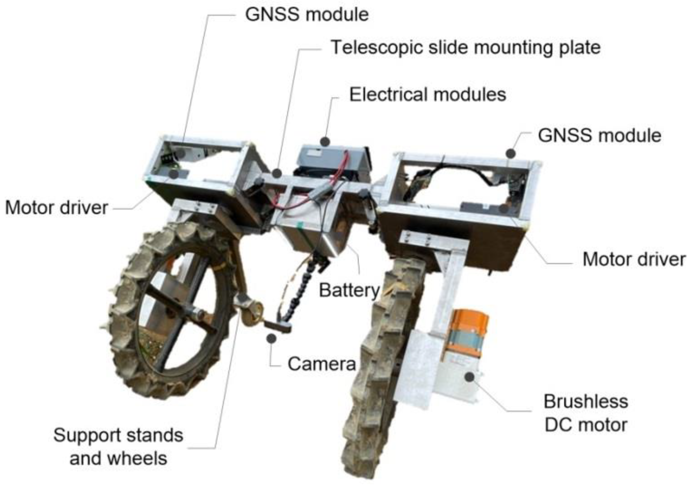
The appearance of a two-wheeled robot trailer (which had a length (L) × width (W) × height (H) of 132 cm × 92 cm × 87.5 cm) is shown in
Figure 1.
Table 1 represents the specifications of the hardware and mechanism components of the robot trailer. The auxiliary wheel was 6 inches (15 cm) in diameter and was attached to the bottom of the support frame (50 cm in length). The left and right sides of a piece of aluminum alloy plate, whose length could be adjusted, were connected to the left and right brackets of the robot, respectively. A brushless DC motor (Model: 9B200P-DM, TROY Enterprise Co., Ltd., New Taipei City, Taiwan) was selected as the power source for the two-wheeled robot trailer. The rated speed, torque, and maximum torque of the motor were 3000 rpm, 0.8 N-m, and 1.0 N-m, respectively. The gear ratio of the reducer was 36, and the transmission efficiency was 80%. The bearing of the reducer was connected to the wheel through a ball bearing seat.
GNSS modules and motor drivers were installed in the left and right frames of the robot, and electrical modules, including the image-processing board and guidance control board, were mounted on the aluminum alloy plate. The rack under the aluminum alloy plate was used to place the battery. A tube was clamped to the rack. The end of the tube was connected to a camera module (Model: Logitech BRIO, Logitech International S.A., Lausanne, Switzerland). The driver could output 0~24 VDC, the power was 200 W, and it supports the communication specifications of RS-232 and RS-485. The size of the battery pack was 22 (L) cm × 16 (W) cm × 11 (H) cm, which could output 24 V/30 Ah. The direct current (DC)-to-DC module could step down the output voltage of the battery pack from 24 V to 5 V, thereby supplying power to electrical modules and others.
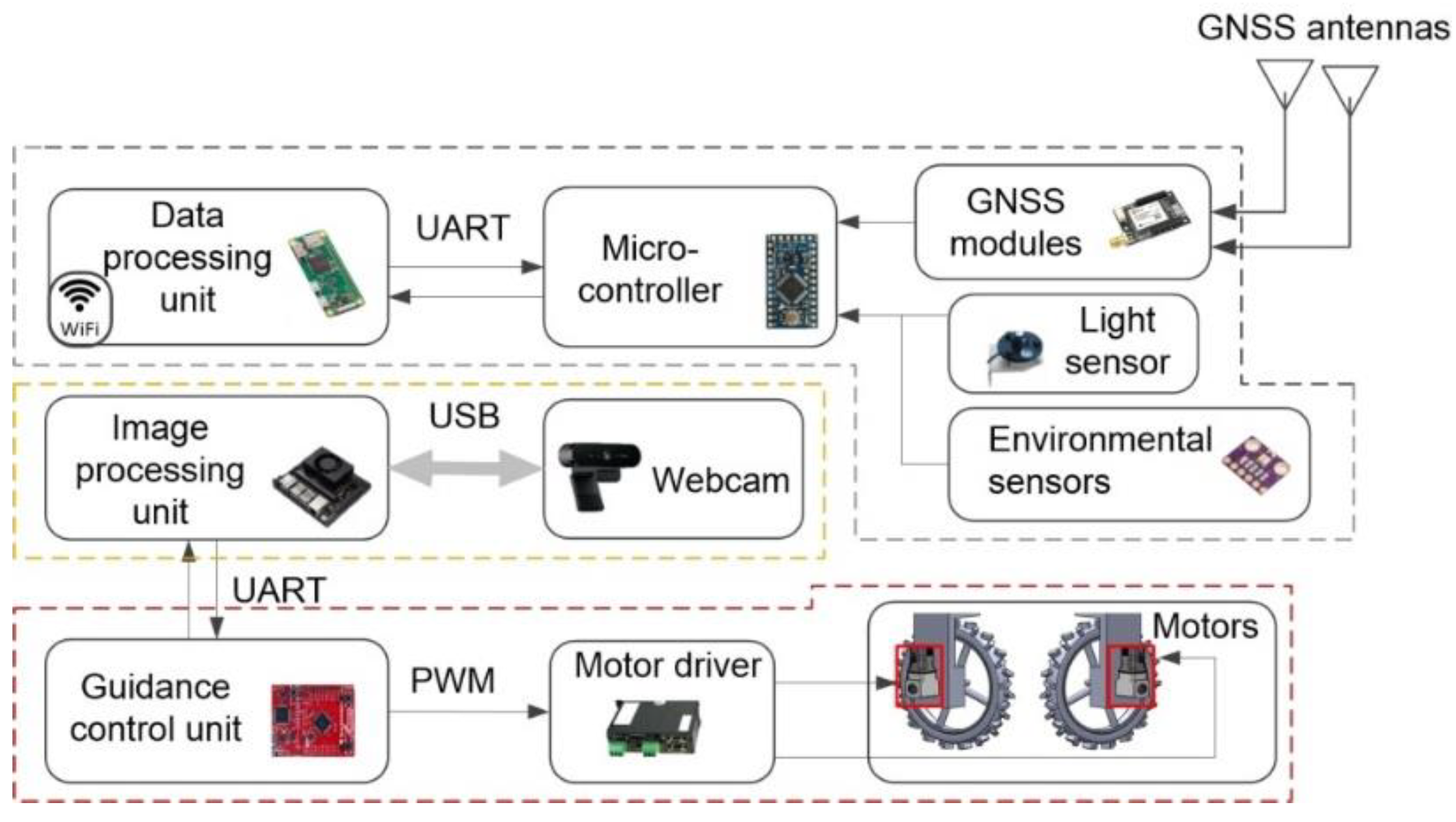
The architecture of the guidance and control system is shown in
Figure 2. A GNSS module (Model: F9P, u-blox Company, Thalwil, Switzerland) with antennas was utilized to determine the location of the robot. The location data were transmitted from the GNSS module via a universal asynchronous receiver/transmitter (UART) interface to the microcontroller, which also received the sensing data obtained by the optical quantum meter and the environmental sensor. The location and sensing data were transmitted to the data processing unit through UART, and the data processing unit transmitted these data to the local server for storage through WiFi.
The images captured by the camera module were sent to the image-processing unit (Model: Xarier NX, NVIDIA Company, Santa Clara, CA, USA), which performed a drip tape detection algorithm to estimate the deviation angle. After that, this deviation angle value was transmitted to the steering control unit (Model: EK-TM4C123GXL, TI Company, Dallas, TX, USA) via UART, and then the built-in steering control program of the unit was executed to estimate the drive voltages of left and right wheel motor. Finally, the voltage value was converted into a pulse width modulated (PWM) signal and sent to a motor driver (Model: BLD-350-A, Zi-Sheng Company, Taichung City, Taiwan) to drive the two motors.
2.2. Drip Tape Following Approach
This section presents the kinematic model of a two-wheeled robot trailer in a Cartesian coordinate frame under nonholonomic constraints, and the drip-tape-following methods are also illustrated in this section.
2.2.1. Kinematic Model
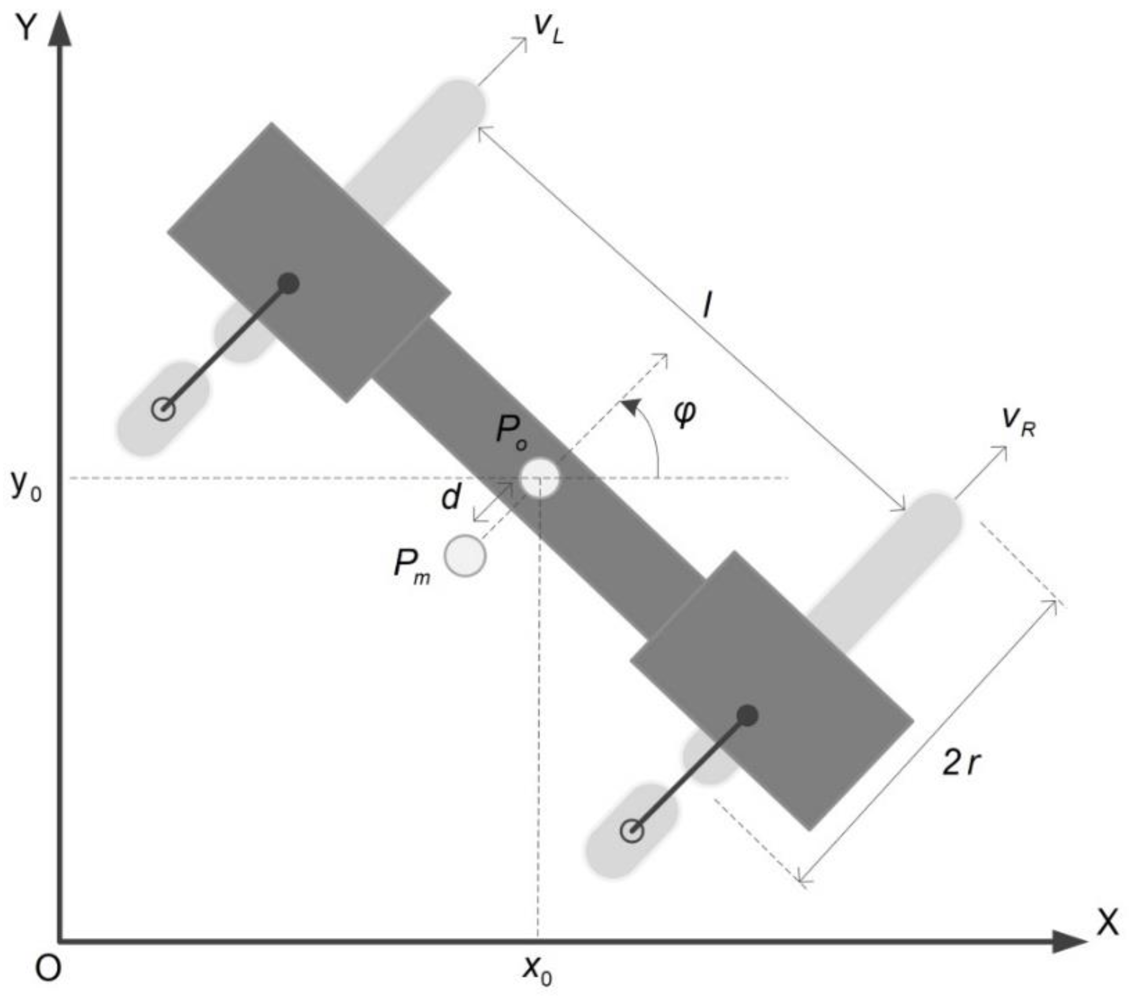
The two wheels of the robot were actuated on a plane by two independent motors, which provide torque to the two wheels. The radius of the two wheels was assumed to be
, and the distance between the two wheels was
. The pose of the robot in the inertial Cartesian frame {O-X-Y} could be described by the position
and the orientation angle
measured relative to the X-axis, which is represented in
Figure 3. The symbol
represented the center of mass of the two-wheeled robot, and its distance from point
was
. Assuming that the velocities in the X-axis and Y-axis directions of
were
and
, respectively; the angular velocity was
; and the sideslip was ignored, the kinematics model of the robot under constraint conditions could be defined as follows [
52,
53]:
where
and
represented the volocities of the left and right wheels of the robot, respectively.
2.2.2. Drip Tape Detection
This section presented the detection methods of drip irrigation tapes, including two edge detection methods (Canny and Laplacian) and the proposed approach. Simple examples were also presented.
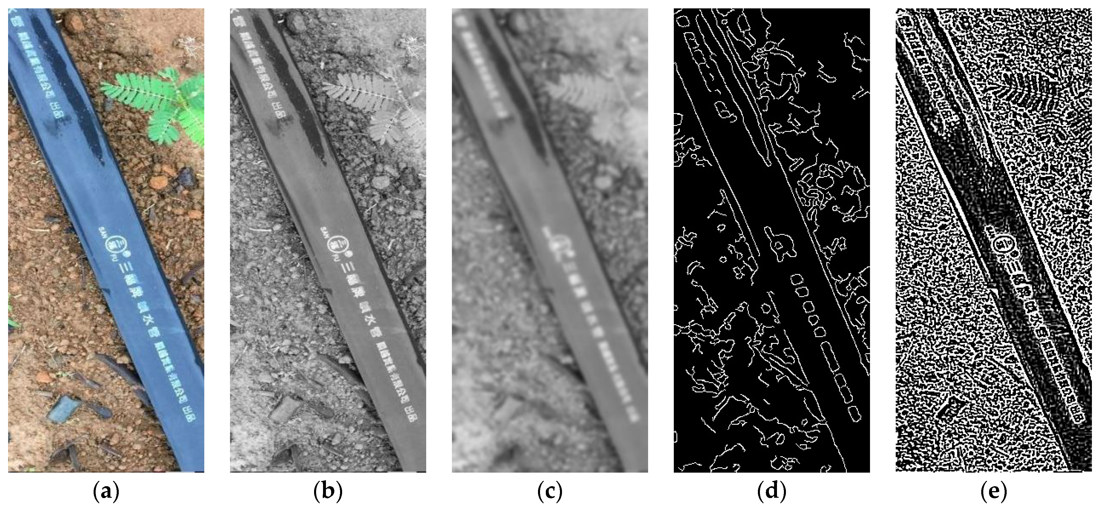
The premise of implementing this method was to first convert the red (R)-green (G)-blue (B) (RGB) color space of the original digital image (
Figure 4a) into grayscale (
Figure 4b) and then perform a Gaussian blur on the image (
Figure 4c). Its main purpose was to reduce the effect of noise components on edge detection. Next, assume the first-order derivatives in the horizontal and vertical directions within the image, which were denoted as
and
, respectively, as in Equations (2) and (3):
where Sobel operators
and
were designed to maximize the response to edges running vertically and horizontally with respect to the pixel grid. The operator consists of a pair of 3 × 3 convolution masks. The masks could be employed individually to the input image, which produce separate measurements of the gradient components in each direction.
indicated the measured pixel grids in the image. The symbol “
“ depicted the convolution operator.
These two gradient components could then be combined together to learn the absolute magnitude
of the gradient at each point and the direction of its gradient (see Equation (4)). The angle of the directional gradients could also be measured by Equation (5):
Nonmaximum suppression was used to remove the blurred gradient values of edge detection pixel grids. The main concept of this method was to compare the gradient intensity of the current pixel with the intensity values of two pixels along the positive and negative gradient directions of the point. If the gradient value of the current pixel was greater than the gradient values of the other two pixels, the current pixel was reserved as an edge point; otherwise, the value of the pixel point was discarded.
Next, a double threshold was used to find some potential edge pixels caused by noise and color changes. True weak edge points could be preserved by suppressing weak edge pixels extracted from noise/color variations. The result of edge detection is shown in
Figure 4d.
The Laplacian-based edge detector used only one kernel to compute the second derivative of the image. It was also necessary to convert the RGB color space of the digital image into grayscale. Before performing Laplacian edge detection, the Gaussian blur operation was employed to reduce the influence of non-dominant features on detected objects, such as noise. Then, Equation (6) was utilized to find the edge points in the image:
where
represented the Laplacian operator. After the Laplacian operation, the median filter was also used to filter out spot noise in the image, so that the edges could be represented very clearly. The edge detection results obtained in
Figure 4c using the Laplacian method with a median filter was shown in
Figure 4e.
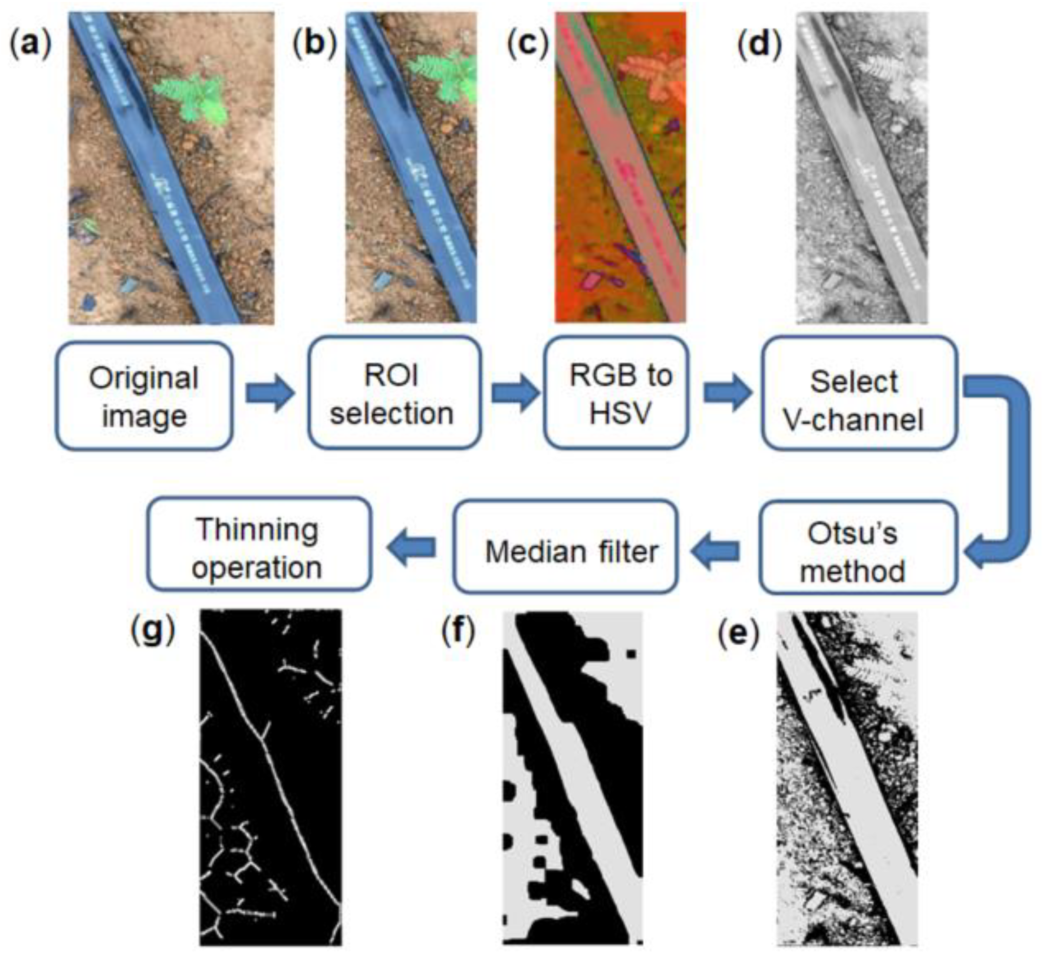
It was difficult to observe the brightness, saturation, and hue of the object pixels in the digital image based on the RGB model. Therefore, the HSV model was used to replace the original RGB model. Assume an 8-bit digital image was captured by a camera. The image was cropped into an ROI of L× width (Q), which could be regarded as a two-dimensional matrix, and the R, G, and B channels presented in each pixel
,
, and
in the matrix were divided. Each of the color channels represented
,
, and
, and these values were between 0 and 255:
where
,
. Operators
and
represented the selection of the maximum and minimum values, respectively. For example,
Figure 5a,b are the original RGB image and the ROI, respectively. The ROI image was converted from the RGB model to the HSV model via Equation (7) (see
Figure 5c).
For an image with a uniform gray distribution, the larger the variance value was, the larger the difference was between the two parts in the image. Otsu’s method utilized the maximum interclass variance that was relatively common as a measure of classification criteria. This method was used to separate the background and objects in the V-channel of the HSV image (see
Figure 5d). Using threshold segmentation to maximize the interclass variance means that the probability of misclassification was minimized. Assume
N represents the total number of pixels in an ROI of the image depicted in Equation (8):
where
(
) illustrated the number of pixels whose gray values were
, and
denoted the maximum gray level of the ROI in the image. The probability of gray level
of pixel occurrence was depicted by
. The threshold
could be employed to divide the gray level of the image into two groups:
and
. The grayscale numbers of
and
were
and
, respectively. Then,
and
were the probabilities of the two groups. The means of
and
were depicted as
and
, respectively. The mean value of gray level over the whole image was
. For any value of
, equations
and
could be easily verified. The variances of
and
were
and
, respectively. The intraclass and interclass variance are shown in Equations (9) and (10), respectively:
The sum of the variance of the intraclass and interclass was
. Therefore, maximizing the interclass variation was equivalent to minimizing the intraclass variation so that the optimal critical threshold
could be obtained as follows:
Each pixel
of the V-channel in the HSV image after execution by Otsu’s method was shown in
Figure 5e, and the image was then denoised (
Figure 5f) and thinned (
Figure 5g).
2.2.3. Hough Transformation
The Hough line transform (HLT) was used to detect the line in the image, which could be presented in the form of
in the Hough space (Hough, 1962).
and
denoted the slope and constant, respectively. There would be an infinite number of lines passing through the edge points
on the edge image, except the vertical line, because
was an undefined value (Leavers, 1992). Therefore, the alternative equation
in the polar coordinate frame was used to replace the original equation. The symbol
represented the shortest length from the origin to the line, and
expressed the angle between the line and horizontal axis. For all values of
, each pixel in the image was mapped to Hough space. Assuming there were two pixels on the same line, their corresponding cosine curves would intersect on a particular
pair. Each pair represented each line that passes by
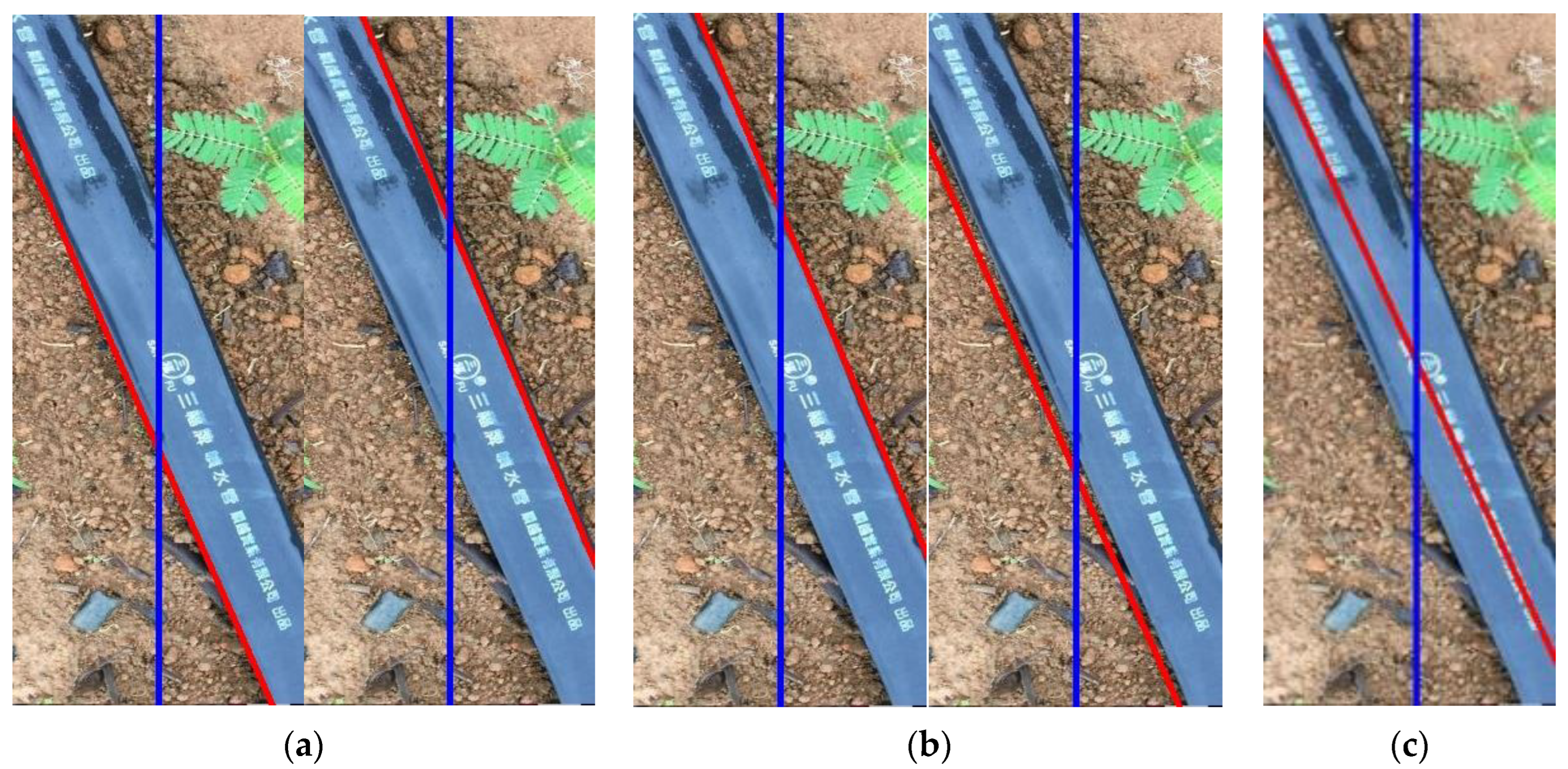
. This detection process was carried out in parameter steps or accumulators, which was a voting process. By finding the highest bin in the parameter space, the most likely line and its geometric definition could be extracted. The results (red lines) of
Figure 4d,e,g processed by HLT, respectively, are shown in
Figure 6a–c.
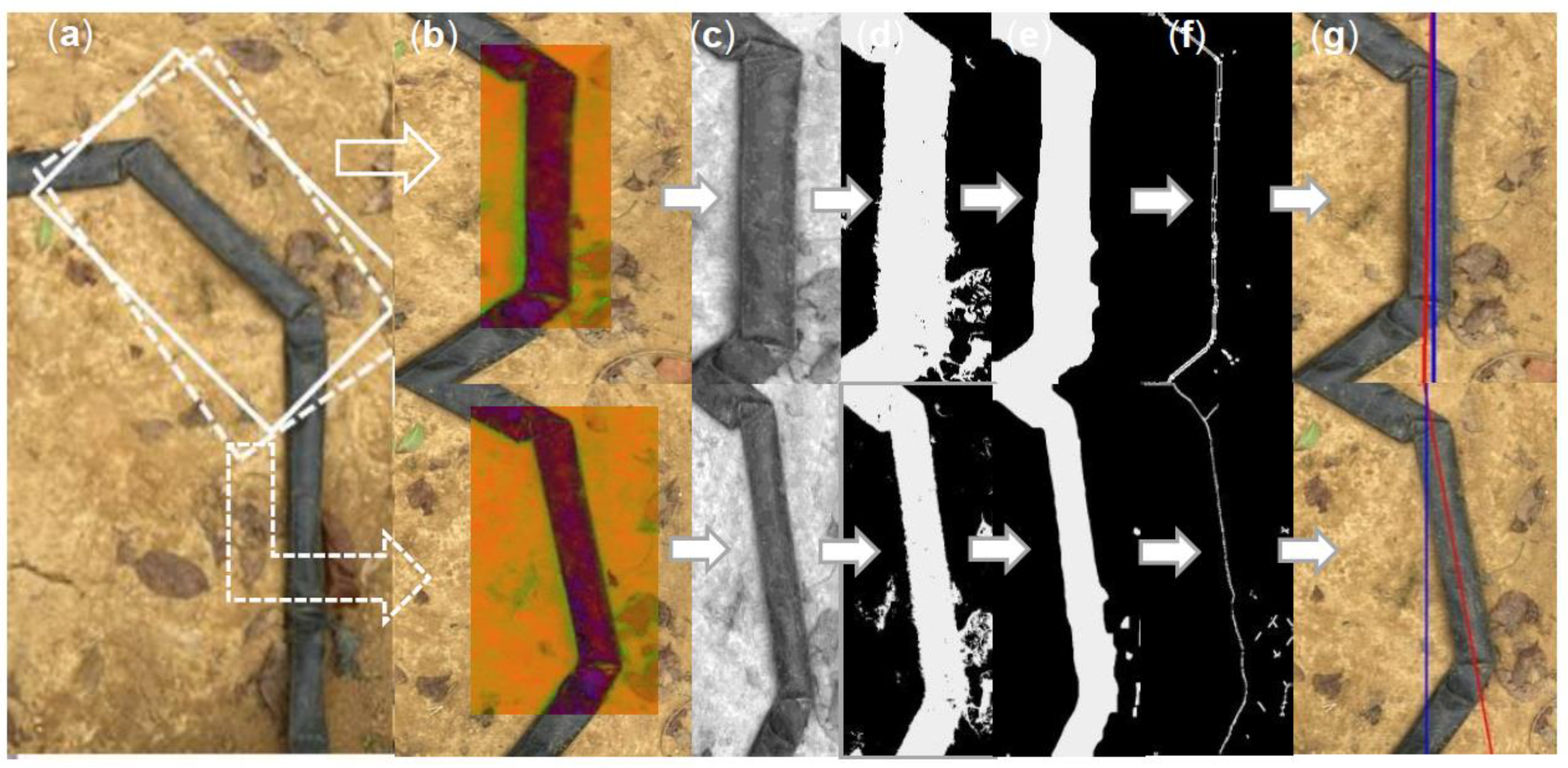
The white solid and dashed frames represented the field of view captured by the camera when the robot turned (
Figure 7a). The upper and lower graphs in
Figure 7b–f represented the image-processing results within the solid frame and the dashed frame, respectively. A line (
Figure 7g) could be obtained by applying the HLT in
Figure 7f.
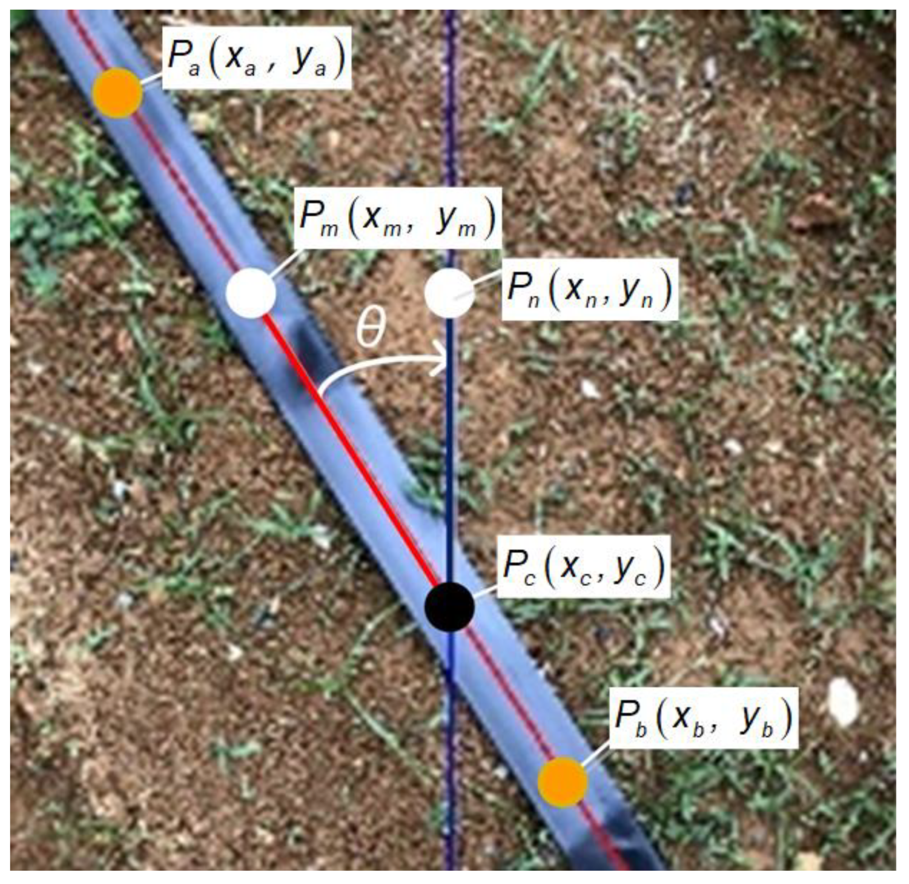
2.3. Determination of the Deviation Angle
Once the drip tape was detected (as shown in the red line in
Figure 8), two points
and
were selected on the red line. At the same time, a vertical line (blue color) was drawn in the center of the image. The blue line intersected the red line at point
. Next, taking a point
on the line segment
, the point horizontally extended a line segment, and the vertical blue line intersected at point
, where
. After obtaining the length of
, the deviation angle
between the drip tape and the centerline of the image could be obtained. When
, the robot heading was parallel to the drip tape.
2.4. Heading Angle Control
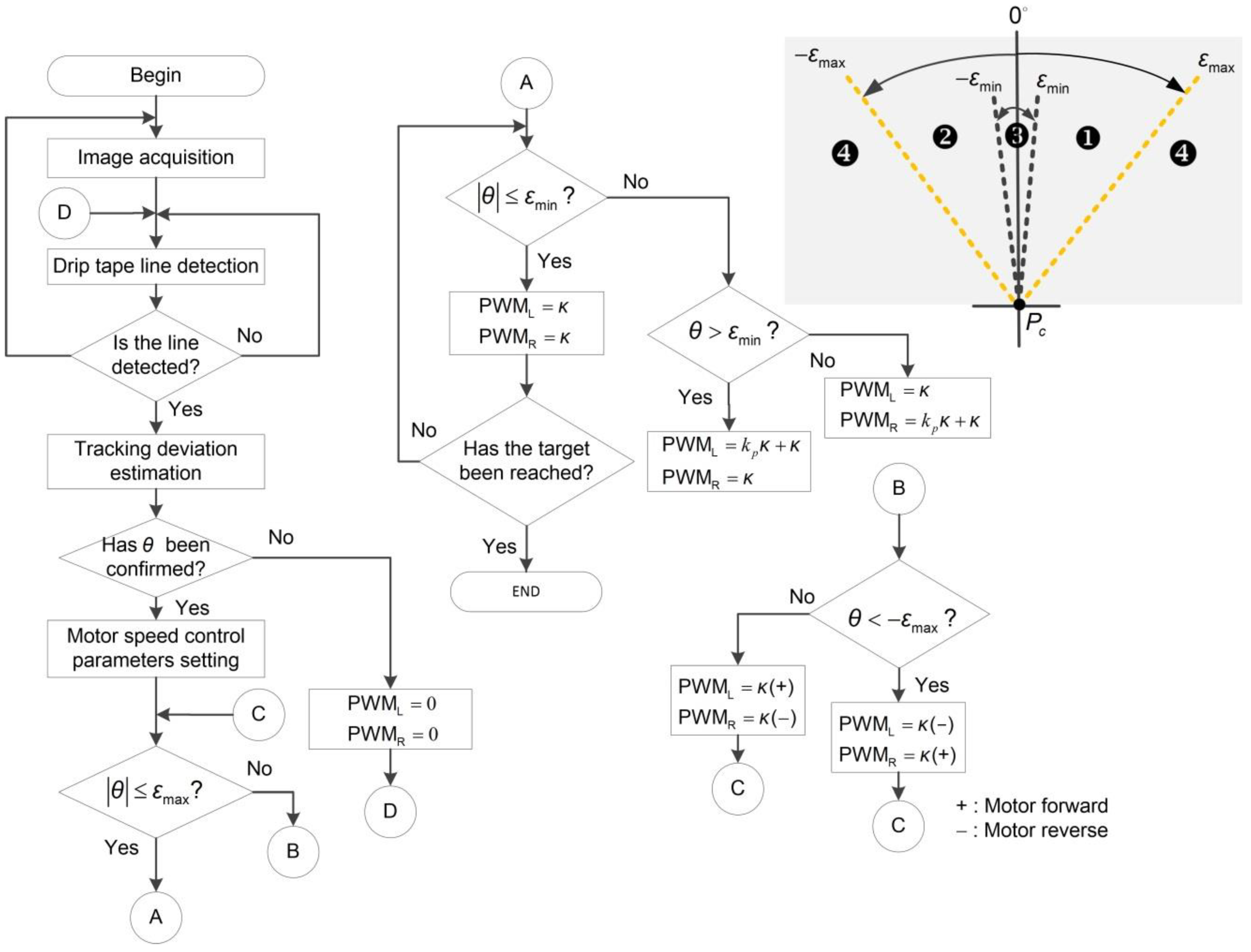
The field navigation mode of the robot was divided into straight forward and turning. A flow chart of the path following control was demonstrated in
Figure 8. First, the digital RGB image was captured by the camera module, the lines in the image were extracted by drip tape detection algorithms (
Section 2.2), and a deviation angle estimation method (described in
Section 2.3) was used to estimate the heading angle. Then, set the PWM value
, the motor speed control gain
, the minimum threshold
, and the maximum threshold
of the heading angle, etc. When
, that is, in the area of “❶” or “❷” or “❸” (see the top right of
Figure 9), the speed difference control was executed. If
, that is, in the “❸” area, then the left and right motor speed control parameters, denoted as
and
, respectively, were equal. Finally, the robot stopped when it moved to the target position. Conversely, when
and
(the area of “❶”), then
and
; in contrast, when
(the area of “❷”), then
and
. When
, it means that
was in the “❹” area, and the steering control program would be executed. When
, set
and
. Conversely, set
and
. Among them, the symbols “+” and “
“ depict the forward rotation and the reverse rotation of the motor, respectively. It was worth noting that the robot stopped (
) once the drip tape was not extracted or an abnormal deviation angle was acquired.
3. Experimental Results
This section illustrates different drip tape detection methods for testing and verification of two-wheeled robot trailers in the field. The performance comparison, analysis, and discussion of different drip tape following methods are also presented in this section.
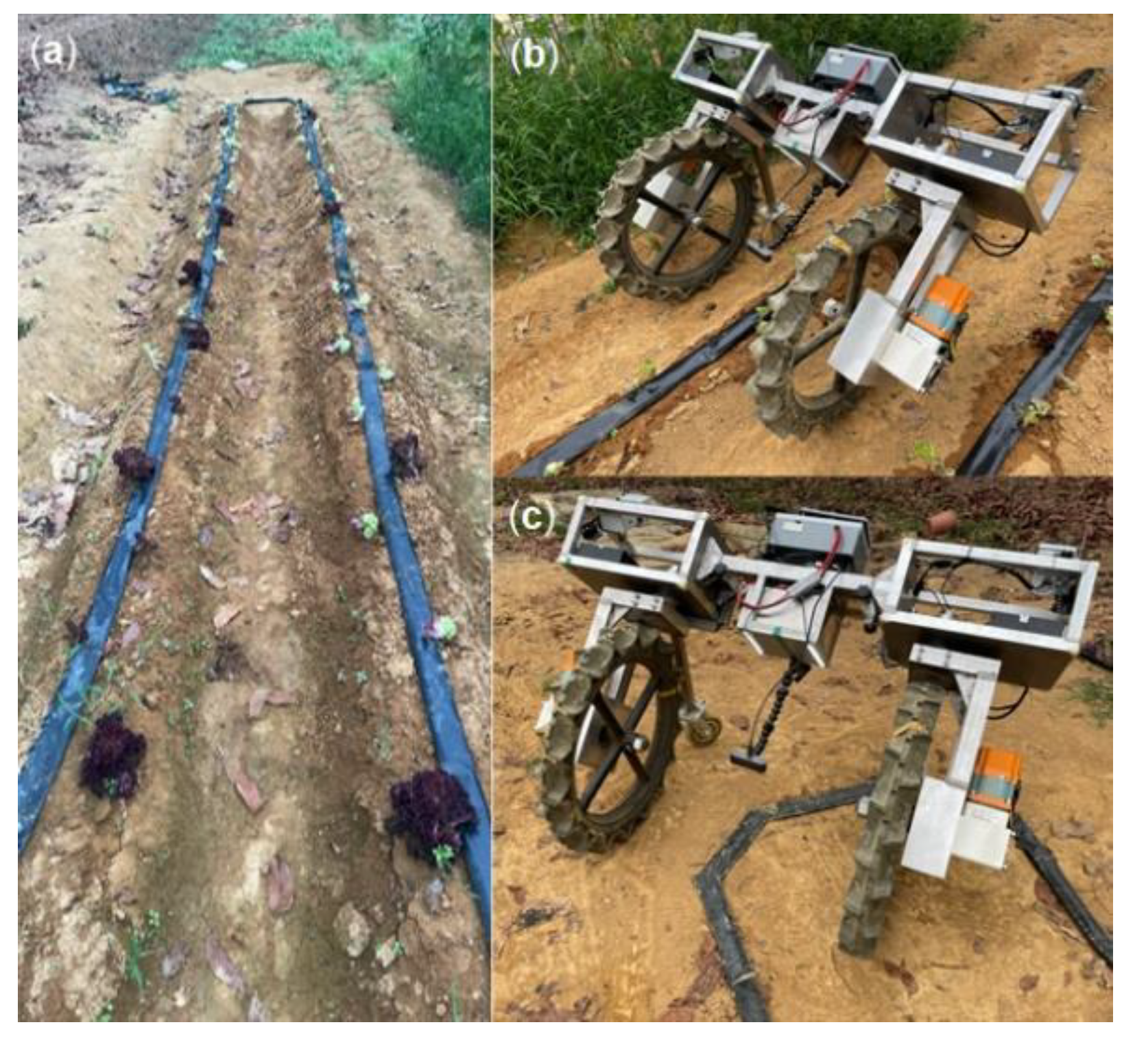
The experimental site was located in front of the experimental factory of the Department of Biomechatronics Engineering of Pingtung University of Science and Technology (Longitude: 120.60659 Latitude: 22.64606). The field had a size of L × W × H of 10 × 0.25 × 0.2 m (see
Figure 10a). The experiment was carried out during the spring, and the weather conditions were mostly cloudy and sunny in the morning and cloudy in the afternoon. According to the climate conditions, butter lettuce (LS-047, Known-You Seed Co., Ltd., Kaohsiung, Taiwan) and red lettuce (HV-067, Known-You Seed Co., Ltd., Kaohsiung, Taiwan) were selected for planting in the field. A black drip tape was laid on the field. The robot would continuously follow the drip tape and move to another tape area (see
Figure 10b,c). The control parameters of the motors were set to
and
. The image processing speed was 5 fps.
and
were set to
and
degrees, respectively.
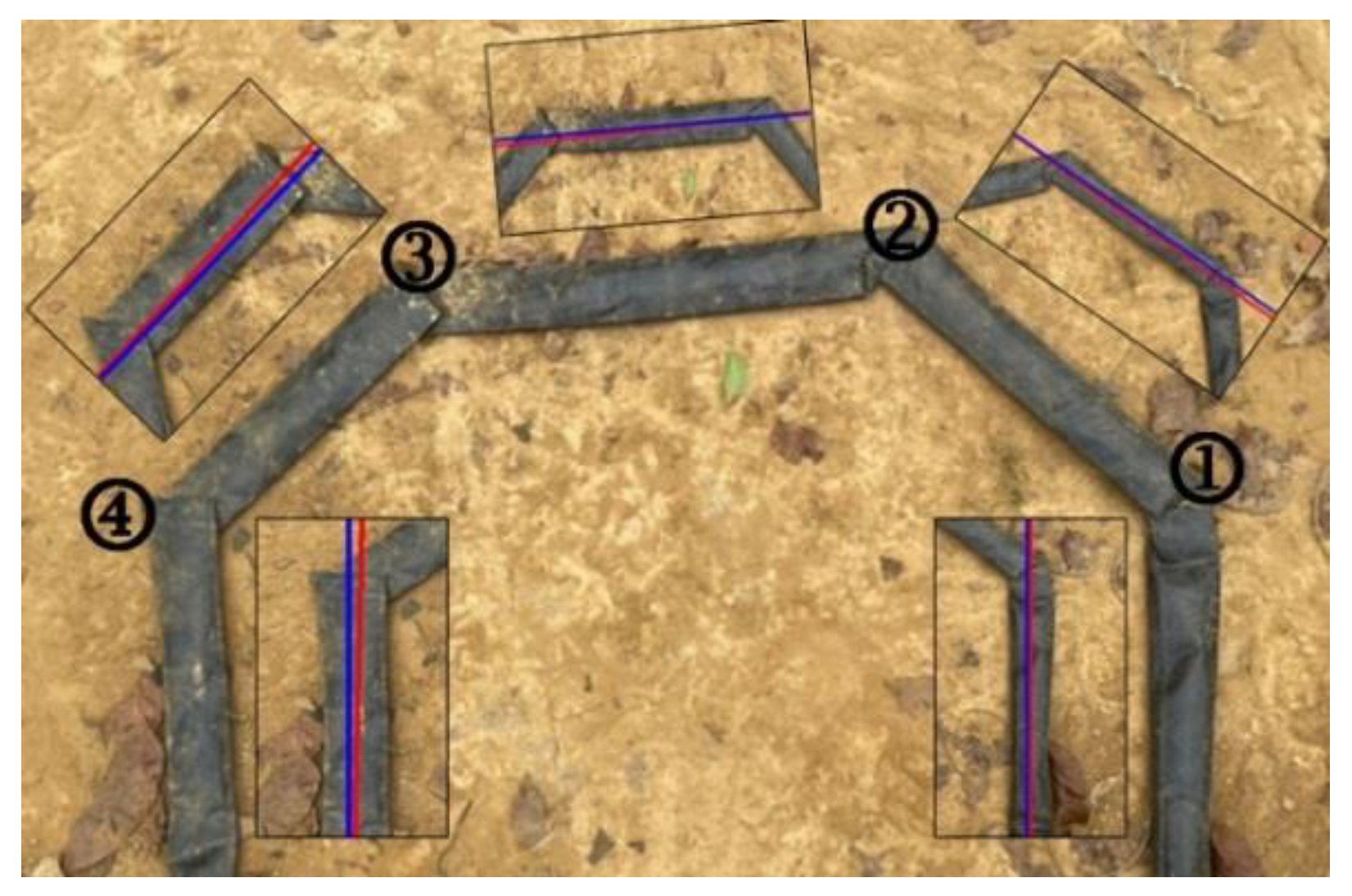
The drip tape was configured as a polygon in the turning area. As shown in
Figure 11, there were four corner points, which were represented as “①”, “②”, “③”, and “④”. This figure also showed the drip tape detection results for each segment (red line within a black box).
Then, the guiding performance of the robot was tested. The test duration was from 6:00 in the morning to 10:00 in the evening, which was divided into eight time intervals, and the robot followed the drip tape to rewind the field twice in each time interval. During the experiment, the line detection rate, , was estimated. Among them, and represented the total number of processed images and the number of images that successfully detected the drip tape in the test duration of each interval, respectively. Finally, the average detection rate of the line could be obtained, and denoted the total number of test durations. The processing rate of the image was 20 fps.
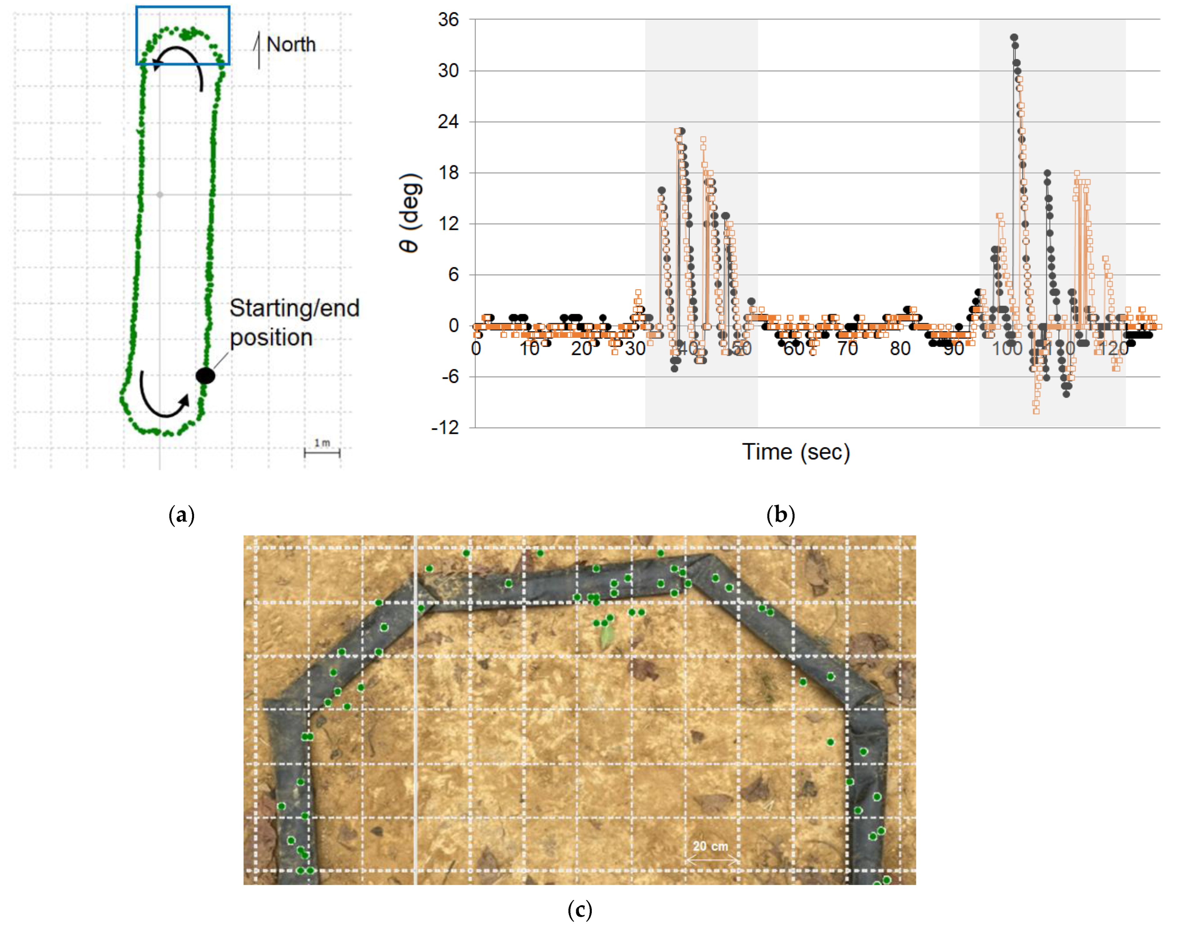
Figure 12a presents the movement trajectory of the robot obtained by the GNSS-RTK positioning module at 06:00 in the morning using the proposed-HLT; the heading angle of the robot (the first loop: black-dot color; the second loop: brown hollow-dot color) was also shown in
Figure 12b. The gray area represents the variation in heading angle when the robot turns. The movement trajectory of the robot during the turning process was shown in the blue box in
Figure 12a, which was enlarged in
Figure 12c (green color).
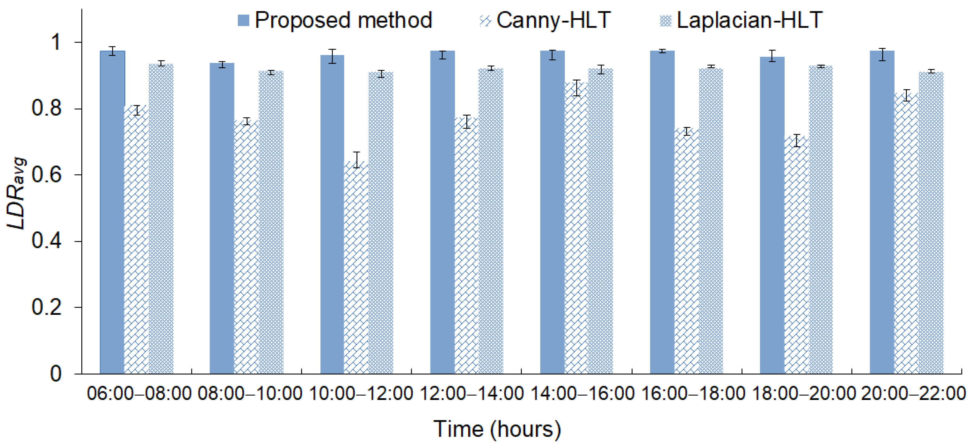
Similarly, two drip tape detection methods based on Canny and Laplacian combined with HLT (called Canny-HLT and Laplacian-HLT) were used to conduct the above experiments and evaluate the performance of different drip tape detection methods. The performance test was repeated for three days (
), and the results are shown in
Figure 13. The average line detection rates obtained by the Canny-HLT, Laplacian-HLT, and proposed-HLT methods in different time intervals were 65~84%, 91~93%, and 93~97%, respectively.
During the experiment, the guiding performance for following straight and polyline trajectories was evaluated with a total length of 44 m.
Table 2 presents the evaluation results of the robot’s guidance performance, including the mean maximum error (MAE), maximum lateral error (ME), and root mean square error (RMSE). The MAE of the proposed-HLT was 2.6 ± 1.1 cm, which was lower than that of the Canny-HLT method (3.2 ± 1.2 cm) and the Laplacian-HLT (2.9 ± 1.6 cm). When using the Canny-HLT method, the robot has the largest ME when moving in a straight line, which reaches 12.3 cm. Using the proposed-HLT results in the smallest RMSE of 2.9 cm in total traveling length. A video of experimental results is demonstrated in
Supplementary material.
4. Discussion
The proposed-HLT has been verified to obtain an average LDR of 96.6% under the condition of unstable light intensity outdoors. Select the V-channel of the HSV image for drip tape detection, which could reduce the brightness and contrast of the image to enhance the differences between objects and backgrounds in the image. The experimental results demonstrated that the LDR during the daytime was at least 93.8%. It was worth noting that the LED lighting device installed on the robot could be used at night (20:00–22:00), and the results depicted that the LDR during this time interval could reach 97.5%. In sunny and cloudless summer conditions, the image would be overexposed due to excessive light and cause a failed recognition result. Therefore, once the drip tape was not detected or an abnormal deviation angle was estimated, the robot would stop. The robot did not start moving until the deviation angle was confirmed and the drip tape line has been extracted. Therefore, once the planting season comes to summer, the safety of the robot during the movement could still be guaranteed under uncertain climatic factors.
The drip tape detection performance using the Canny-HLT was the worst among the three methods. Since the Canny algorithm has its own execution flow, it was difficult to use it with other image-processing algorithms, which also limits its flexibility in use. For images with uniform grayscale variation, it was hard to detect boundaries by only using the first derivative (such as the Canny operation). At this time, the use of a second derivative operation could provide critical information, such as the Laplacian operation. This method was often used to determine whether the edge pixels in the image were bright or dark areas. By smoothing the image to reduce noise, the Laplacian method could also achieve a detection rate of up to 93.4% after combining with Hough line transformation. Compared with the Canny-HLT method, the detection performance of the Laplacian-HLT method was more stable.
When the Canny-HLT or Laplacian-HLT program was executed in the high-speed embedded system, lines on the left or right side of the drip tape were detected (
Figure 7a,b) under the condition of an image processing speed of 7 fps. The line segment of drip tape detected first would be used for heading angle estimation.
The configuration of the drip tape as a polygon allowed the robot to perform the U-turning operation smoothly, and a larger ROI could prevent the intersection of the line segment and the vertical line from falling outside the ROI. At this time, it would also cause three line segments to appear at the same time in the ROI of the image (as shown in the black frame in
Figure 11), which indirectly increased the probability of misjudgment of the heading angle. Therefore, the estimated angle was checked by monitoring the variation in the heading angle to ensure the stability of the robot’s traveling. This configuration of the drip tape could enable the robot trailer to move autonomously and turn to another narrow strip. This study only investigated a drip tape line detection operation based on mathematical morphology and Hough transformation, which was used in complex environments and unstable light intensity conditions. Once the detected target or object characteristics change, the parameters of the proposed approach need to be adjusted specifically. In principle, the color of the drip tape was different from that of most soils (except for black soils). Generally speaking, the material was very suitable for two-wheeled robots to be used as object tracking. Although green crops could also be selected as objects, different types of crops have different characteristics and sizes, and the planting interval of each crop would also be adjusted according to the size of the crop. Due to the many factors or parameters to be considered, the object detection process would be more complicated.
On the other hand, although the color of the soil was similar to that of the drip tape, fortunately, the surface of the drip tape and the soil were still different in brightness under uniform lighting. Therefore, using Otsu’s binarization method could still distinguish the foreground object from the background. Using a drip tape that was similar in color to the soil was undesirable when working in the field. Secondly, the recognition performance of the proposed solution was limited by the existence of shadows in the objects in the image. Therefore, it was more suitable to use the proposed approach when there were no shelters (such as trees) around the field.
When using deep learning for object detection, its detection performance was limited by the diversity of images and the number of labeled samples used in model training [
54]. Once the experimental site was changed or the climate changes (such as solar radiation), the images to be identified have to be collected again and the detection model has to be rebuilt. In addition, the operation of labeling target objects was also time-consuming.
The advantage of using image processing was that it could only extract the features of the target object in the image, especially the objects with obvious features. However, this detection method is limited by the image quality and the high complexity of the feature extraction would indirectly increase the computational load. These problems have been solved due to the gradual improvement in camera hardware level, the gradual popularization of high-speed computing processors, and reduction in costs.
The proposed robot trailer adopted differential speed steering control, which has a small turning radius and was suitable for fields with narrow planting spacing and turning areas. In addition, deep tread tires could repel mud, which could be used on sticky soils or upland fields. The narrow tire could reduce the friction between the tire and the ground, making the steering control more flexible.
During the experiment, although the drip tape in some areas was blocked by mud or weeds, the proposed approach could successfully detect the line of drip tape. In addition, during drip irrigation, the drip tape would be filled with water, and the appearance would expand slightly, but it has no effect on the line detection for the robot trailer.
5. Conclusions
The proposed machine-vision-based approach could provide the two-wheeled robot trailer to move along the drip tape in the field. Three line detection methods were used to evaluate the autonomous guiding performance of the robot. Among them, the proposed image recognition strategy could effectively detect the drip tape on the strip-planting area and estimate the angle of heading deviation to make the robot travel stably between planting areas, especially in the case of unstable light conditions.
The robot trailer was small in size, and it was suitable for autonomous guiding operations in 1 hectare fields, especially for strip, till, or no-till farming applications. In the future, the proposed approach would be integrated with deep learning for guideline detection and heading angle control. In addition, the robot would be equipped with a shock absorption device and a steering device, so that the robot has more applications.
Author Contributions
Conceptualization, C.-L.C. and C.-C.Y.; methodology, C.-L.C. and H.-W.C.; software, H.-W.C. and Y.-H.C.; verification, C.-L.C., H.-W.C. and Y.-H.C.; data management, H.-W.C.; writing—manuscript preparation, C.-L.C., H.-W.C. and Y.-H.C.; writing—review and editing, C.-L.C.; visualization, C.-L.C. and Y.-H.C.; supervision, C.-L.C. and C.-C.Y.; project management, C.-L.C.; fund acquisition, C.-L.C. All authors have read and agreed to the published version of the manuscript.
Funding
This research was funded by Ministry of Science and Technology (MOST), Taiwan, grant number MOST 109-2321-B-020-004; MOST 110-2221-E-020-019.
Institutional Review Board Statement
Not applicable.
Informed Consent Statement
Not applicable.
Data Availability Statement
The datasets presented in this study are available from the corresponding author on reasonable request.
Conflicts of Interest
The authors declare no conflict of interest.
References
- McCool, C.; Beattie, J.; Firn, J.; Lehnert, C.; Kulk, J.; Bawden, O.; Russell, R.; Perez, T. Efficacy of mechanical weeding tools: A study into alternative weed management strategies enabled by robotics. IEEE Robot. Autom. Lett. 2018, 3, 1184–1190. [Google Scholar] [CrossRef]
- Hemming, J.; Nieuwenhuizen, A.T.; Struik, L.E. Image analysis system to determine crop row and plant positions for an intra-row weeding machine. In Proceedings of the CIGR International Symposium on Sustainable Bioproduction, Tokyo, Japan, 19–23 September 2011; pp. 1–7. [Google Scholar]
- Xiong, Y.; Ge, Y.; Liang, Y.; Blackmore, S. Development of a prototype robot and fast path-planning algorithm for static laser weeding. Comput. Electron. Agric. 2017, 142, 494–503. [Google Scholar] [CrossRef]
- Peruzzi, A.; Martelloni, L.; Frasconi, C.; Fontanelli, M.; Pirchio, M.; Raffaelli, M. Machines for non-chemical intra-row weed control in narrow and wide-row crops: A review. J. Agric. Eng. 2017, 48, 57–70. [Google Scholar] [CrossRef] [Green Version]
- Chang, C.L.; Lin, K.M. Smart agricultural machine with a computer vision-based weeding and variable-rate irrigation scheme. Robotics 2018, 7, 38. [Google Scholar] [CrossRef] [Green Version]
- Chang, C.L.; Xie, B.X.; Chung, S.C. Mechanical control with a deep learning method for precise weeding on a farm. Agriculture 2021, 11, 1049. [Google Scholar] [CrossRef]
- Astrand, B.; Baerveldt, A.J. An agricultural mobile robot with vision-based perception for mechanical weed control. Auton. Robots 2002, 13, 21–35. [Google Scholar] [CrossRef]
- Emmi, L.; Le Flecher, E.; Cadenat, V.; Devy, M. A hybrid representation of the environment to improve autonomous navigation of mobile robots in agriculture. Precis. Agric. 2021, 22, 524–549. [Google Scholar] [CrossRef]
- Opiyo, S.; Okinda, C.; Zhou, J.; Mwangi, E.; Makange, N. Medial axis-based machine-vision system for orchard robot navigation. Comput. Electron. Agric. 2021, 185, 106153. [Google Scholar] [CrossRef]
- Grimstad, L.; From, P.J. The Thorvald II agricultural robotic system. Robotics 2017, 6, 24. [Google Scholar] [CrossRef] [Green Version]
- Reiser, D.; Sehsah, E.-S.; Bumann, O.; Morhard, J.; Griepentrog, H.W. Development of an autonomous electric robot implement for intra-row weeding in vineyards. Agriculture 2019, 9, 18. [Google Scholar] [CrossRef] [Green Version]
- Fue, K.G.; Porter, W.M.; Barnes, E.M.; Rains, G.C. An extensive review of mobile agricultural robotics for field operations: Focus on cotton harvesting. AgriEngineering 2020, 2, 150–174. [Google Scholar] [CrossRef] [Green Version]
- Yin, X.; Du, J.; Geng, D. Development of an automatically guided rice transplanter using RTKGNSS and IMU. IFAC PapersOnline 2018, 51, 374–378. [Google Scholar] [CrossRef]
- Ng, K.M.; Johari, J.; Abdullah SA, C.; Ahmad, A.; Laja, B.N. Performance evaluation of the RTK-GNSS navigating under different landscape. In Proceedings of the 18th International Conference on Control, Automation and Systems (ICCAS), PyeongChang, Korea, 17–18 October 2018; pp. 1424–1428. [Google Scholar]
- Mutka, A.; Miklic, D.; Draganjac, I.; Bogdan, S. A low cost vision based localization system using fiducial markers. IFAC PapersOnline 2008, 41, 9528–9533. [Google Scholar] [CrossRef] [Green Version]
- Byun, Y.S.; Kim, Y.C. Localization based on magnetic markers for an all-wheel steering vehicle. Sensors 2016, 16, 2015. [Google Scholar] [CrossRef] [PubMed] [Green Version]
- Chen, Y.-R.; Chao, K.; Kim, M.S. Machine vision technology for agricultural applications. Comput. Electron. Agric. 2002, 36, 173–191. [Google Scholar] [CrossRef] [Green Version]
- Perez, L.; Rodriguez, I.; Rodriguez, N.; Usamentiaga, R.; Garcia, D.F. Robot guidance using machine vision techniques in industrial environments: A Comparative Review. Sensors 2016, 16, 335. [Google Scholar] [CrossRef]
- Kuruvilla, J.; Sukumaran, D.; Sankar, A.; Joy, S.P. A review on image processing and image segmentation. In Proceedings of the 2016 International Conference on Data Mining and Advanced Computing (SAPIENCE), Ernakulam, India, 16–18 March 2016; pp. 198–203. [Google Scholar] [CrossRef]
- Malik, M.H.; Zhang, T.; Li, H.; Zhang, M.; Shabbir, S.; Saeed, A. Mature tomato fruit detection algorithm based on improved HSV and watershed algorithm. IFAC PapersOnline 2018, 51, 431–436. [Google Scholar] [CrossRef]
- Wu, X. Review of theory and methods of image segmentation. Agric. Biotechnol. 2018, 7, 136–141. [Google Scholar]
- Preetha, M.M.S.J.; Suresh, L.P.; Bosco, M.J. Image segmentation using seeded region growing. In Proceedings of the 2012 International Conference on Computing, Electronics and Electrical Technologies (ICCEET), Nagercoil, India, 21–22 March 2012; pp. 576–583. [Google Scholar]
- Otsu, N. A threshold selection method from gray-level histograms. IEEE Trans. Syst. Man Cybern. 1979, 9, 62–66. [Google Scholar] [CrossRef] [Green Version]
- Haralick, R.M.; Shapiro, L.G. Image segmentation techniques. Comput. Gr. Image Process. 1985, 29, 100–132. [Google Scholar] [CrossRef]
- Marr, D.; Hildreth, E. Theory of edge detection. Proc. R. Soc. Lond. B Biol. Sci. 1980, 207, 187–217. [Google Scholar] [CrossRef] [PubMed]
- Canny, J.A. computational approach to edge detection. IEEE PAMI 1986, 8, 679–714. [Google Scholar] [CrossRef]
- Kaganami, H.G.; Beij, Z. Region based segmentation versus edge detection. In Proceedings of the 2009 Fifth International Conference on Intelligent Information Hiding and Multimedia Signal Processing, Kyoto, Japan, 12–14 September 2009; pp. 1217–1221. [Google Scholar]
- Al-Amri, S.S.; Kalyankar, N.; Khamitkar, S. Image segmentation by using edge detection. Int. J. Comput. Sci. Eng. Technol. 2010, 2, 804–807. [Google Scholar]
- Wang, H.; Ying, D. An improved image segmentation algorithm based on OTSU method. Comput. Simul. 2011, 6625, 262–265. [Google Scholar]
- Huang, M.; Yu, W.; Zhu, D. An improved image segmentation algorithm based on the Otsu method. In Proceedings of the 13th ACIS International Conference on Software Engineering, Artificial Intelligence, Networking and Parallel/Distributed Computing, Kyoto, Japan, 8–10 April 2012; pp. 135–139. [Google Scholar]
- Huang, C.; Li, X.; Wen, Y. An OTSU image segmentation based on fruitfly optimization algorithm. Alex. Eng. J. 2021, 60, 183–188. [Google Scholar] [CrossRef]
- Wu, Z.; Leahy, R. An optimal graph theoretic approach to data clustering: Theory and its application to image segmentation. IEEE Trans. Pattern Anal. Mach. Intell. 1993, 15, 1101–1113. [Google Scholar] [CrossRef] [Green Version]
- Celebi, M.E.; Kingravi, H.A.; Vela, P.A. A comparative study of efficient initialization methods for the kmeans clustering algorithm. Expert Syst. Appl. 2013, 40, 200–210. [Google Scholar] [CrossRef] [Green Version]
- Dhanachandra, N.; Manglem, K.; Chanu, Y.J. Image segmentation using k-means clustering algorithm and subtractive clustering algorithm. Procedia Comput. Sci. 2015, 54, 764–771. [Google Scholar] [CrossRef] [Green Version]
- Zheng, X.; Lei, Q.; Yao, R.; Gong, Y.; Yin, Q. Image segmentation based on adaptive k-means algorithm. Eurasip J. Image Video Process. 2018, 1, 68. [Google Scholar] [CrossRef]
- Srinivasan, V.; Bhatia, P.; Ong, S.H. Edge detection using a neural network. Pattern Recognit. 1994, 27, 1653–71662. [Google Scholar] [CrossRef]
- Sowmya, B.; Rani, B.S. Colour image segmentation using fuzzy clustering techniques and competitive neural network. Appl. Soft Comput. 2011, 11, 3170–3178. [Google Scholar] [CrossRef]
- Sultana, F.; Sufian, A.; Dutta, P. Evolution of image segmentation using deep convolutional neural network: A survey. Knowl. Based Syst. 2020, 201, 106062. [Google Scholar] [CrossRef]
- Kukolj, D.; Marinovic, I.; Nemet, S. Road edge detection based on combined deep learning and spatial statistics of LiDAR data. J. Spat. Sci. 2021, 1–15. [Google Scholar] [CrossRef]
- Xue, J.; Zhang, L.; Grift, T.E. Variable field-of-view machine vision based row guidance of an agricultural robot. Comput. Electron. Agric. 2012, 84, 85–91. [Google Scholar] [CrossRef]
- Li, N.L.; Zhang, C.; Chen, Z.; Ma, Z.; Sun, Z.; Yuan, T.; Li, W.; Zhang, J. Crop positioning for robotic intra-row weeding based on machine vision. IJABE 2015, 8, 20–29. [Google Scholar]
- Pajares, G.; Garcia-Santillan, I.; Campos, Y.; Montalvo, M.; Guerrero, J.M.; Emmi, L.; Romeo, J.; Guijarro, M.; Gonzalez-de-Santos, P. Machine-vision systems selection for agricultural vehicles: A Guide. J. Imaging 2016, 2, 34. [Google Scholar] [CrossRef] [Green Version]
- Shrivakshan, G.T.; Chandrasekar, C. A comparison of various edge detection techniques used in image processing. Int. J. Comput. Sci. Issues IJCSI 2012, 9, 269. [Google Scholar]
- Torii, T.; Kitade, S.; Teshima, T.; Okamoto, T.; Imou, K.; Toda, M. Crop row tracking by an autonomous vehicle using machine vision (part 1): Indoor experiment using a model vehicle. J. JSAM 2000, 62, 41–48. [Google Scholar]
- Bak, T.; Jakobsen, H. Agricultural robotic platform with four wheel steering for weed detection. Biosyst. Eng. 2004, 87, 125–136. [Google Scholar] [CrossRef]
- Leemans, V.; Destain, M.F. Application of the hough transform for seed row localisation using machine vision. Biosyst. Eng. 2006, 94, 325–336. [Google Scholar] [CrossRef] [Green Version]
- Bakker, T.; Wouters, H.; van Asselt, K.; Bontsema, J.; Tang, L.; Muller, J.; van Straten, G. A vision based row detection system for sugar beet. Comput. Electron. Agric. 2008, 60, 87–95. [Google Scholar] [CrossRef]
- Ponnambalam, V.R.; Bakken, M.; Moore, R.J.D.; Gjevestad, J.G.O.; From, P.J. Autonomous crop row guidance using adaptive multi-ROI in strawberry fields. Sensors 2020, 20, 5249. [Google Scholar] [CrossRef] [PubMed]
- Rabab, S.; Badenhorst, P.; Chen, Y.P.P.; Daetwyler, H.D. A template-free machine vision-based crop row detection algorithm. Precis. Agric. 2021, 22, 124–153. [Google Scholar] [CrossRef]
- Ma, Z.; Tao, Z.; Du, X.; Yu, Y.; Wu, C. Automatic detection of crop root rows in paddy fields based on straight-line clustering algorithm and supervised learning method. Biosyst. Eng. 2021, 211, 63–76. [Google Scholar] [CrossRef]
- De Silva, R.; Cielniak, G.; Gao, J. Towards agricultural autonomy: Crop row detection under varying field conditions using deep learning. arXiv 2021, arXiv:2109.08247. [Google Scholar]
- Oriolo, G.; De Luca, A.; Vendittelli, M. WMR control via dynamic feedback linearization: Design, implementation, and experimental validation. IEEE Trans. Control Syst. Technol. 2002, 10, 835–852. [Google Scholar] [CrossRef]
- Chwa, D. Robust distance-based tracking control of wheeled mobile robots using vision sensors in the presence of kinematic disturbances. IEEE Trans. Ind. Electron. 2016, 63, 6172–6183. [Google Scholar] [CrossRef]
- Li, J.; Zhang, D.; Ma, Y.; Liu, Q. Lane image detection based on convolution neural network multi-task learning. Electronics 2021, 10, 2356. [Google Scholar] [CrossRef]
Figure 1.
Appearance of the two-wheeled robot trailer.
Figure 1.
Appearance of the two-wheeled robot trailer.
Figure 2.
The guidance and control system architecture for a two-wheeled robot trailer.
Figure 2.
The guidance and control system architecture for a two-wheeled robot trailer.
Figure 3.
The representation of the position and orientation of the two-wheeled robot in the Cartesian coordinate system. Dark gray, light gray, and black color represent the mechanism body, wheels, and support stands, respectively.
Figure 3.
The representation of the position and orientation of the two-wheeled robot in the Cartesian coordinate system. Dark gray, light gray, and black color represent the mechanism body, wheels, and support stands, respectively.
Figure 4.
Process flow of edge detection: (a) original image; (b) grayscale; (c) Gaussian blur; (d) Canny edge detection; (e) Laplacian edge detection.
Figure 4.
Process flow of edge detection: (a) original image; (b) grayscale; (c) Gaussian blur; (d) Canny edge detection; (e) Laplacian edge detection.
Figure 5.
Drip tape extraction process: (a) Original image; (b) ROI image; (c) HSV image; (d) V-channel; (e) Otsu’s binarization method; (f) median filter; (g) thinning operation.
Figure 5.
Drip tape extraction process: (a) Original image; (b) ROI image; (c) HSV image; (d) V-channel; (e) Otsu’s binarization method; (f) median filter; (g) thinning operation.
Figure 6.
Results of different drip tape detection methods combined with HLT (red color): (a) Canny with HLT; (b) Laplacian with HLT; (c) proposed HLT.
Figure 6.
Results of different drip tape detection methods combined with HLT (red color): (a) Canny with HLT; (b) Laplacian with HLT; (c) proposed HLT.
Figure 7.
Line detection result when the robot turned: (a) Two frames within the snapshot that require image processing (solid frame and dashed frame); (b) The result of HSV transformation of the ROI in the solid frame (top) and the dashed frame (bottom) in the image (a); (c) The V channel of the HSV image; (d) Binarization; (e) Median filtering; (f) Thinning; (g) Hough line transformation (red line) and the central vertical line (blue) of the image.
Figure 8.
The deviation of heading angle estimation (red line: desired line; blue line: vertical line in the center of the image; white dotted line: horizontal line in the center of the image).
Figure 8.
The deviation of heading angle estimation (red line: desired line; blue line: vertical line in the center of the image; white dotted line: horizontal line in the center of the image).
Figure 9.
Line of drip tape detection and steering control process. The numbers “❶”, “❷”, “❸” and “❹” respectively demonstrated the areas corresponding to the heading of the robot; the letters A, B, C, D inside the circle represented flowchart connectors.
Figure 9.
Line of drip tape detection and steering control process. The numbers “❶”, “❷”, “❸” and “❹” respectively demonstrated the areas corresponding to the heading of the robot; the letters A, B, C, D inside the circle represented flowchart connectors.
Figure 10.
The appearance of experimental field and the two-wheeled robot: (a) the appearance of the field; (b) the snapshot of the two-wheeled trailer traveling autonomously; (c) the U-turning process of the robot trailer.
Figure 10.
The appearance of experimental field and the two-wheeled robot: (a) the appearance of the field; (b) the snapshot of the two-wheeled trailer traveling autonomously; (c) the U-turning process of the robot trailer.
Figure 11.
The configuration of the drip tape in the turning area and its detection result (red line). The blue line represented the vertical line in the center of the image. The numbers “①”, “②”, “③”, and “④” represented the corner points, which can divide the drip tape into five line segments.
Figure 11.
The configuration of the drip tape in the turning area and its detection result (red line). The blue line represented the vertical line in the center of the image. The numbers “①”, “②”, “③”, and “④” represented the corner points, which can divide the drip tape into five line segments.
Figure 12.
The movement trajectory and deviation angle of the robot (test time interval: 06:00–08:00 a.m.): (a) Movement trajectory of the robot, initial location: 22.64657° N, 120.6060° E (the area of grid: 1 (length) × 1 (width) m); (b) The variation in heading angle when the robot travels (black-dot color: the first loop; brown hollow-dot color: the second loop); (c) The position point (green-dot color) distribution of the moving trajectories of the two loop (the area of grid: 20 (L) × 20 (W) cm).
Figure 13.
Comparison of the drip tape detection performance of the three methods at different time intervals within three days.
Figure 13.
Comparison of the drip tape detection performance of the three methods at different time intervals within three days.
Table 1.
Component specifications for the robot trailer.
Table 1.
Component specifications for the robot trailer.
| Description | Value or Feature |
|---|
| Mechanism body | |
| Size: L [cm] × W [cm] × H [cm] | 132 × 92 × 87.5 |
| Front wheel: D [cm] × W [cm] | 65 × 8 |
| Rear wheel: D [cm] × W [cm] | 15 × 4 |
| Electronics | |
| Data processing board (speed; memory) | 1 GHz single-core ARMv6 CPU (BCM2835); 512 MB RAM |
| Image processing board (speed; memory) | 6-core NVIDIA Carmel ARM; 8 GB LPDDR4x |
| Guidance control board (speed; memory) | ARM Cortex-M processor; 256 KB single-cycle Flash memory |
| Motor (voltage;velocity; gear ratio; power; torque) | 24 V; 3000 rpm; 1:36; 200 W; 0.8 N-m |
| Driver (voltage; power; communication) | 24 V; 200 W; RS-232/RS-485 |
| Camera (connection; resolution; focus) | USB 2.0/3.0; 4096 × 2160 (30 frame per second (fps)); Auto |
| GNSS board (interface; type; voltage; precision) | USB/UART; Multi constellation; 5 V; <4 cm with state space representation (SSR) corrections (precise point positioning (PPP) in Real-Time Kinematic (RTK)). |
| DC–DC module (input voltage; output voltage) | 28 V; 5 V |
| Others | |
| Battery (voltage, capacity) | 24 V; 30 Ah |
| Antennas (type; voltage) | Passive; 3.3 V |
Table 2.
The performance evaluation results of different line detection methods in the guidance system of the robot.
Table 2.
The performance evaluation results of different line detection methods in the guidance system of the robot.
| | Travel Distance (m) | MAE ± SD (cm) | ME (cm) | RMSE (cm) |
|---|
| Canny-HLT | 32 (Straight) | 4.2 ± 1.7 | 12.3 | 5.8 |
| 12 (Polyline) | 2.3 ± 1.4 | 10.7 | 2.7 |
| 44 (Total) | 3.2 ± 1.2 | 11.2 | 3.6 |
| Laplacian-HLT | 32 (Straight) | 3.9± 1.4 | 11.4 | 5.1 |
| 12 (Polyline) | 2.1 ± 1.9 | 7.6 | 2.2 |
| 44 (Total) | 2.9 ± 1.6 | 7.8 | 3.3 |
| Proposed-HLT | 32 (Straight) | 3.6 ± 1.5 | 8.6 | 4.9 |
| 12 (Polyline) | 1.9 ± 1.4 | 6.4 | 1.7 |
| 44 (Total) | 2.6 ± 1.1 | 6.9 | 2.9 |
| Publisher’s Note: MDPI stays neutral with regard to jurisdictional claims in published maps and institutional affiliations. |
© 2022 by the authors. Licensee MDPI, Basel, Switzerland. This article is an open access article distributed under the terms and conditions of the Creative Commons Attribution (CC BY) license (https://creativecommons.org/licenses/by/4.0/).


