
A Stability Analysis Using AΜΜΙ and GGE Biplot Approach on Forage Yield Assessment of Common Vetch in Both Conventional and Low-Input Cultivation Systems

Abstract
:1. Introduction
- (i)
- data quality and methodological approaches in the analysis of yield stability that are as transparent as possible,
- (ii)
- testing for and deal with outliers,
- (iii)
- investigation on potentially confounding factors in the statistical model,
- (iv)
- exploratory pathways on the need for detrending of yield data,
- (v)
- account for temporal autocorrelation,
- (vi)
- the choice for the stability measures and consider the correlation between some of the measures,
- (vii)
- consideration on the dependence of stability measures on the mean yield,
- (viii)
- temporal trends of stability, and
- (ix)
- reports on standard errors and statistical inference of stability measures where possible.
2. Materials and Methods
2.1. Crop Establishment and Experimental Procedures
- (A)
- InGiannitsa, Northern Greece (latitude, 40°77′ N;longitude, 22°39′ E;elevation,10 m a.s.l.). The soil type was clay (C): sand, 9.1%; silt, 37.5%; clay, 53.8%. The chemical properties of the soil were as follows: conventional: N-NO3, 15.1 mg kg−1; P-Olsen, 17.4 mg kg−1; K, 274 mg kg−1; pHH20, 7.69; organic matter, 3.26%; and CaCO3, 5.23(%).Low-input system: N-NO3, 16.1 mg kg−1; P-Olsen, 15.9 mg kg−1; K, 261 mg kg−1; pHH20,7.65; organic matter, 3.51%, and CaCO3, 5.37(%).
- (B)
- In the farm of the Technological Educational Institute of Western Macedonia in Florina, northern Greece (latitude, 40°46′ N;longitude, 21°22′ E;elevation, 705 m a.s.l.). The soil type was characterized as a sandy loam (SL): sand, 62%; silt, 26.9%; clay, 11.1%. The chemical properties of the soil were as follows: conventional: N-NO3, 16.1 mg kg−1; P-Olsen, 26.4 mg kg−1; K, 236 mg kg−1; pHH20, 6.32; organic matter, 1.29%; and CaCO3, 1.7(%). Low-input system: N-NO3, 17.4 mg kg−1; P-Olsen, 25.1 mg kg−1; K, 224 mg kg−1; pHH20,6,29; organic matter, 1.32%, and CaCO3, 1.9(%).
- (C)
- In Trikala, Central, Greece (latitude, 39°55′ N; longitude, 21°64′ E; elevation,120 m a.s.l.). The soil type was characterized as sandy clay loam (SCL): sand, 48.6%; silt, 19.2%; clay, 32.2%. The chemical properties of the soil were as follows: conventional: N-NO3, 12.7 mg kg−1; P-Olsen, 11.8 mg kg−1; K, 168 mg kg−1; pHH20, 8.15; organic matter, 2.21%; and CaCO3, 7.54(%). Low-input system: N-NO3, 13.6 mg kg−1; P-Olsen, 11.5 mg kg−1; K, 176 mg kg−1; pHH20,8.11; organic matter, 2.39%, and CaCO3, 7.63(%).
- (D)
- In Kalambaka, Central Greece (latitude, 39°64′ N;longitude, 21°65′ E;elevation, 190 m a.s.l.). The soil type was silty clay (SiC): sand, 14.6%;silt, 41.2%;clay, 44.2%. The chemical properties of the soil were as follows: conventional: N-NO3, 11.39 mg kg−1; P-Olsen, 7.62 mg kg−1; K, 96.3 mg kg−1; pHH20, 8.05; organic matter, 2.14%; and CaCO3, 3.58(%). Low-input system: N-NO3, 12.01 mg kg−1; P-Olsen, 7.56 mg kg−1; K, 98.7 mg kg−1; pHH20,8.08; organic matter, 2.21%, and CaCO3, 3.65(%).
2.2. Measurements
- Days to 50% flowering: This corresponds to the number of days passing from the sowing date to 50% of the flowering time; it was recorded for each plot [22].
- Main stem length: Corresponds to the mean height of ten random plants of each plot, measured from ground level to the top point with a ruler (1 mm sensitivity) after extending the plants upward at flowering time. The arithmetic mean of the measurements was accepted as the main stem length for each plot.
- The number of main stems per plant: This corresponds to the number of first stems accounted for from the bottom part of the plants in flowering time. The number occurred as an arithmetic mean of values obtained from ten plants of each plot, situated in different parts of the plot
- Fresh forage yield (kg ha−1): Corresponds to the weight of chloromass (fresh forage) obtained from each plot right after harvesting in full flowering time and subsequent calculation on a hectare basis.
- Dry matter yield (kg ha−1): Corresponds to the dry matter percent per plot calculated after fresh forage samples (0.5 Kg), harvested from each experimental plot were placed at 70 °C for 48 h in a drying oven, left to cool, and weighed. Then, dry matter yield was determined for each plot, and the value was converted to a hectare basis.
- Forage dry matter crude protein content (%): Forage dry matter was passed through a 1 mm sieve and subsequently mixed for the analysis. Total N was determined using AOAC Official Method 988.05 [23] and then the total protein content was estimated.
- Ash content (%) of dry matter: Ash was analyzed using AOAC Official Method 942.05 [23].
2.3. Data Analysis
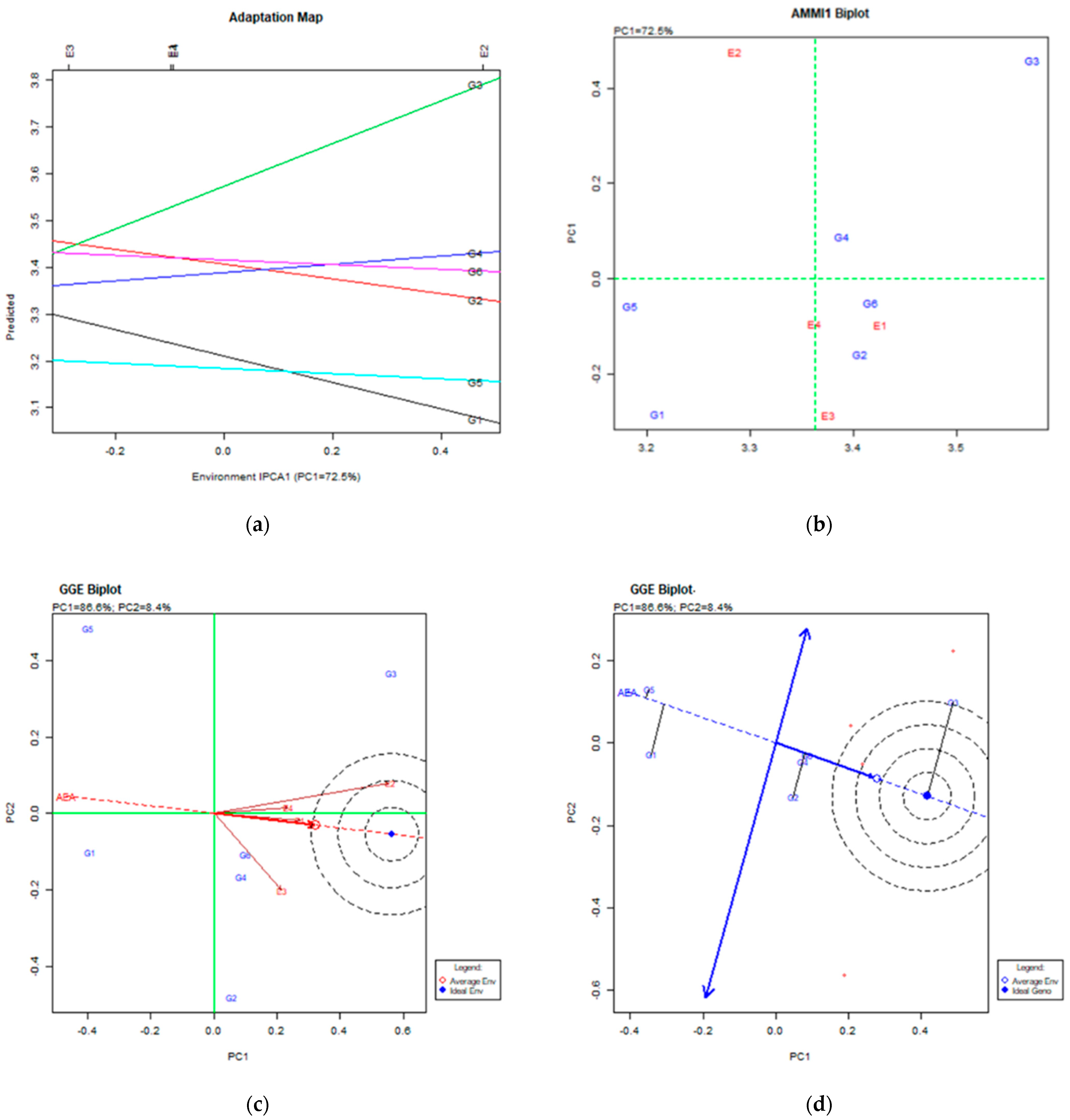
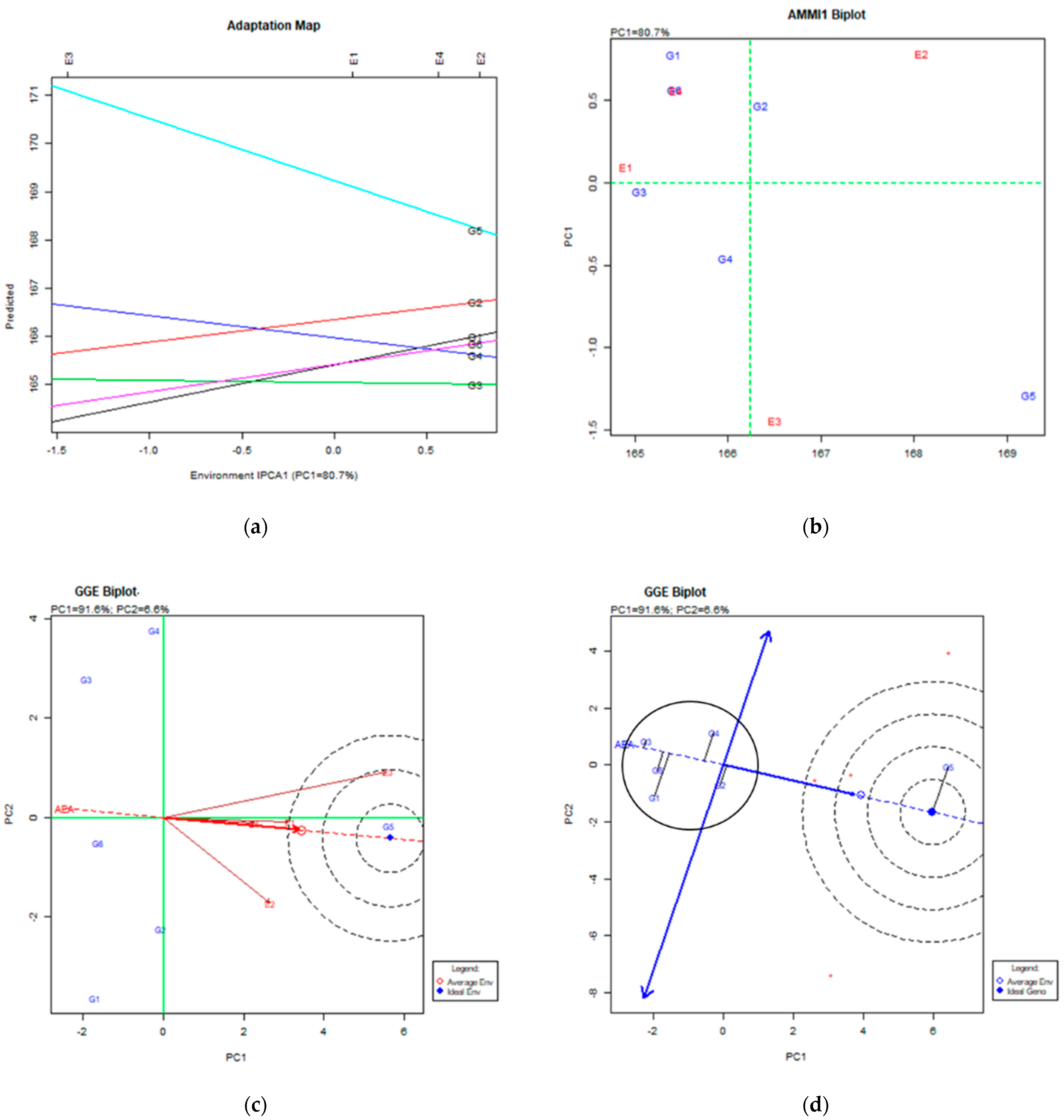
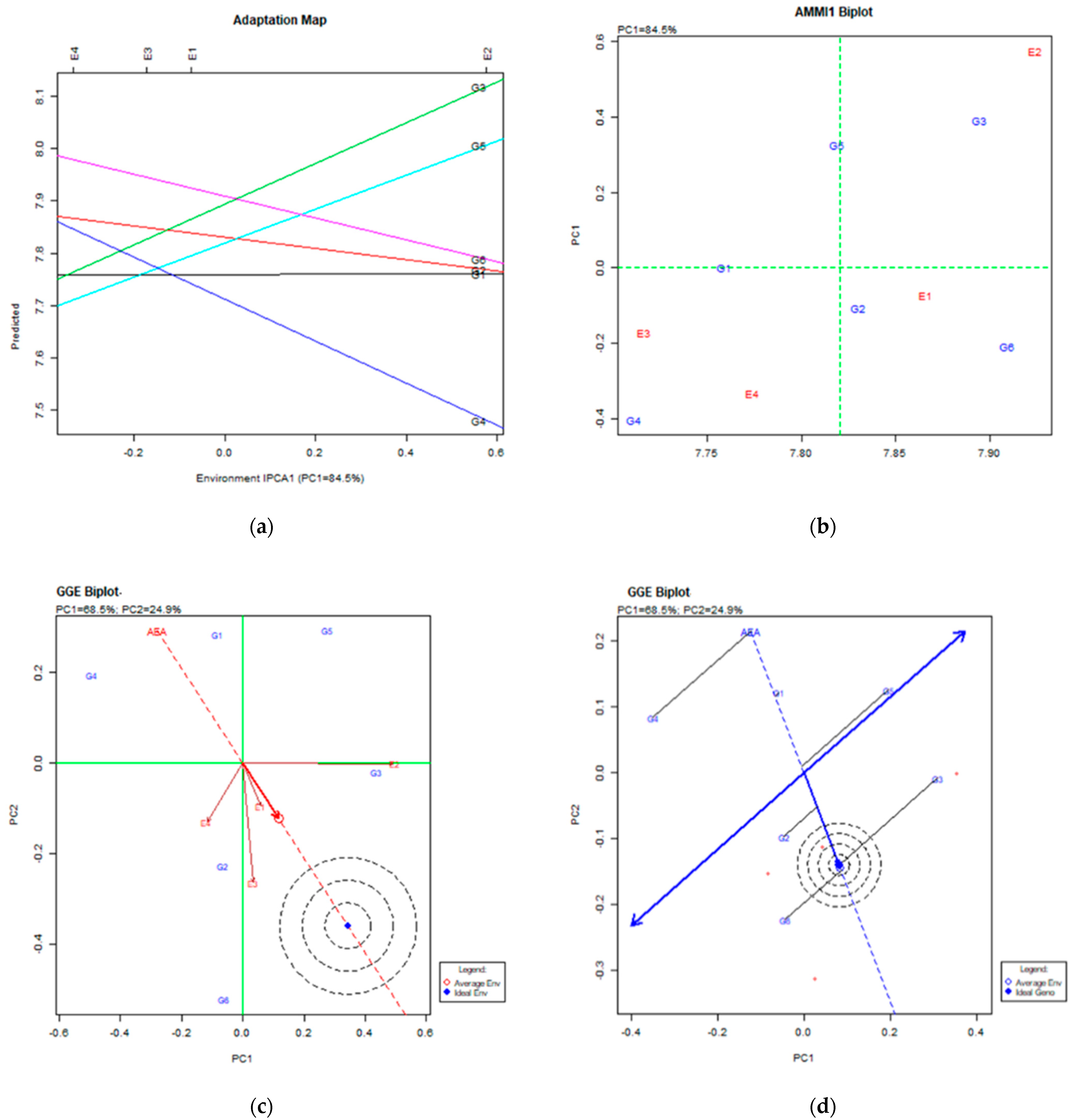
3. Results
Correlations between Characteristics
4. Discussion
4.1. Fresh Forage Yield
4.2. Forage Dry Matter Yield
4.3. Crude Protein Content
4.4. Number of Stems per Plant
4.5. Days to 50% Flowering
4.6. Ash Content
4.7. Correlations between Characteristics
5. Conclusions
Author Contributions
Funding
Institutional Review Board Statement
Informed Consent Statement
Data Availability Statement
Conflicts of Interest
References
- Fırıncıoğlu, H.K.; Erbektas, E.; Doruyol, L.; Mutlu, Z.; Ünal, S.; Karakurt, E. Phenotypic variation of autumn and spring-sown vetch (Vicia sativa ssp.) populations in central Turkey. Span. J. Agric. Res. 2009, 7, 596–606. [Google Scholar] [CrossRef] [Green Version]
- Córdoba, E.M.; Nadal, S.; González-Verdejo, C.I. Common vetch production in Mediterranean Basin. Legume Perspectives. 2015, 10, 34–36. [Google Scholar]
- FAO (Food and Agriculture Organization of the United Nations). FAOSTAT Online Database. 2021. Available online: http://www.fao.org (accessed on 11 April 2021).
- Fırıncıoğlu, H.K.; Tate, M.; Ünal, S.; Doğruyol, S.; Özcan, İ. A selection strategy for low toxin vetches. Turk. J. Agric. For. 2007, 31, 303–311. [Google Scholar]
- Yau, S.K.; Bounejmate, M.; Ryan, J.; Baalbaki, R.; Nassar, A.; Maacaroun, R. Barley–legumes rotations for semi-arid areas of Lebanon. Eur. J. Agron. 2003, 19, 599–610. [Google Scholar] [CrossRef]
- Rinnofner, T.; Friedel, J.K.; de Kruijff, R.; Pietsch, G.; Freyer, B. Effect of catch crops on N dynamics and following crops in organic farming. Agron. Sustain. Dev. 2008, 28, 551–558. [Google Scholar] [CrossRef]
- Vlachostergios, A.; Lithourgidis, A.; Korkovelos, A.; Baxevanos, D.; Lazaridou, T. Mixing ability of conventionally bred common vetch (Vicia sativa L.) cultivars for grain yield under low-input cultivation. Aust. J. Crop Sci. 2011, 5, 1588–1594. [Google Scholar]
- Akdeniz, H.; Koc, A.; Islam, M.S.; El Sabagh, A. Performances of hairy vetch varieties under different locations of mediterranean environment. Fresen. Environ. Bull. 2018, 27, 4263–4269. [Google Scholar]
- Georgieva, N.; Nikolova, I.; Delchev, G. Response of spring vetch (Vicia sativa L.) to organic production conditions. Bulg. J. Agric. Sci. 2020, 26, 520–526. [Google Scholar]
- Fasoula, V.A. A novel equation paves the way for an everlasting revolution with cultivars characterized by high and stable crop yield and quality. In Proceedings of the 11th National Hellenic Conference in Genetics and Plant Breeding, Orestiada, Greece, 31 October–2 November 2006; pp. 7–14. [Google Scholar]
- Fasoula, V.A. Selection of High Yielding Plants Belonging to Entries of High Homeostasis Maximizes Efficiency in Maize Breeding. In Proceedings of the XXI International Eucarpia Conference in Maize and Sorghum Breeding in the Genomics Era, Bergamo, Italy, 21–24 June 2009; p. 29. [Google Scholar]
- Papastylianou, P.; Vlachostergios, D.N.; Dordas, C.; Tigka, E.; Papakaloudis, P.; Kargiotidou, A.; Pratsinakis, E.; Koskosidis, A.; Pankou, C.; Kousta, A.; et al. Genotype x environment interaction analysis of faba bean (viciafaba l.) for biomass and seed yield across different environments. Sustainability 2021, 13, 2586. [Google Scholar] [CrossRef]
- Fasahat, P.; Rajabi, A.; Mahmoudi, S.B.; Noghabi, M.A.; Rad, J.M. An overview on the use of stability parameters in plant breeding. Biom. Biostat. Int. J. 2015, 2, 1–11. [Google Scholar] [CrossRef] [Green Version]
- Reckling, M.; Ahrends, H.; Chen, T.-W.; Eugster, W.; Hadasch, S.; Knapp, S.; Laidig, F.; Linstädter, A.; Macholdt, J.; Piepho, H.P.; et al. Methods of yield stability analysis in long-term field experiments. A review. Agron. Sustain. Dev. 2021, 41, 27. [Google Scholar] [CrossRef]
- Mirosavliević, M.N.; Pržulj, N.; Čanak, P. Analysis of new experimental barley genotype performance for grain yield using AMMI Biplot. Sel. I Semen. 2014, 20, 27–36. [Google Scholar] [CrossRef]
- Hongyu, K.; Garcıa-Pena, M.; de Araujo, L.B.; dos Santos Dias, C.T. Statistical analysis of yield trials by AMMI analysis of genotype × environment interaction. Biom. Lett. 2014, 51, 89–102. [Google Scholar] [CrossRef] [Green Version]
- Asfaw, A.; Alemayehu, F.; Gurum, F.; Atnaf, M. AMMI and SREG GGE biplot analysis for matching varieties onto soybean production environments in Ethiopia. Sci. Res. Essay 2009, 4, 1322–1330. [Google Scholar]
- Fasoulas, A.C. The Honeycomb Methodology of Plant Breeding; Aristoteles University of Thessaloniki: Thessaloniki, Greece, 1988. [Google Scholar]
- Fasoula, V.A. Prognostic breeding: A new paradigm for crop improvement. Plant Breed. Rev. 2013, 37, 297–347. [Google Scholar]
- Greveniotis, V.; Sioki, E.; Ipsilandis, C.G. Estimations of fibre trait stability and type of inheritance in cotton. Czech J. Genet. Plant Breed. 2018, 54, 190–192. [Google Scholar] [CrossRef] [Green Version]
- Hellenic Agricultural Organization Demeter. Ellinikes Pikilies Ktinotrofikon Psihanthon (Greek Varieties of Forage Legumes); Institute of Industrial and Forage Crops: Larissa, Greece, 2015. [Google Scholar]
- Fehr, W.R.; Caviness, C.E. Stages of Soybean Development; Iowa State University: Ames, IA, USA, 1977. [Google Scholar]
- AOAC. Official Methods of Analysis, 18th ed.; Association of Official Analytical Chemists: Gaithersburg, MD, USA, 2005. [Google Scholar]
- Steel, R.G.D.; Torrie, H.; Dickey, D.A. Principles and Procedures of Statistics. A Biometrical Approach, 3rd ed.; McGraw-Hill: New York, NY, USA, 1997. [Google Scholar]
- Koundinya, A.V.V.; Ajeesh, B.R.; Hegde, V.; Sheela, M.N.; Mohan, C.; Asha, K.I. Genetic parameters, stability and selection of cassava genotypes between rainy and water stress conditions using AMMI, WAAS, BLUP and MTSI. Sci. Hortic. 2021, 281, 109949. [Google Scholar]
- Phelan, P.; Moloney, A.P.; McGeough, E.J.; Humphreys, J.; Bertilsson, J.; O’Riordan, E.G.; O’Kiely, P. Forage legumes for grazing and conserving in ruminant production systems. Crit. Rev. Plant Sci. 2015, 34, 281–326. [Google Scholar] [CrossRef]
- Mikó, P.; Löschenberger, F.; Hiltbrunner, J.; Aebi, R.; Megyeri, M.; Kovács, G.; Molnár-Láng, M.; Vida, G.; Rakszegi, M. Comparison of bread wheat varieties with different breeding origin under organic and low input management. Euphytica 2014, 199, 69–80. [Google Scholar] [CrossRef] [Green Version]
- Aydemir, S.K.; Karakoy, T.; Kokten, K.; Nadeem, M.A. Evaluation of yield and yield components of common vetch (Vicia sativa L.) genotypes grown in different locations of Turkey by GGE biplot analysis. Appl. Ecol. Environ. Res. 2019, 17, 15203–15217. [Google Scholar] [CrossRef]
- Sayar, M.S. Additive main effects and multiplicative interactions (ammi) analysis for fresh forage yield in common vetch (vicia sativa l.) genotypes. Agric. For. 2017, 63, 119–127. [Google Scholar]
- Tiryaki, G.Y.; Cil, A.; Tiryaki, I. Revealing seed coat colour variation and their possible association with seed yield parameters in common vetch (Vicia sativa L.). Int. J. Agron. 2016, 2016, 1804108. [Google Scholar]
- Greveniotis, V.; Bouloumpasi, E.; Zotis, S.; Korkovelos, A.; Ipsilandis, C.G. Assessment of interactions between yield components of common vetch cultivars in both conventional and low-input cultivation systems. Agriculture 2021, 11, 369. [Google Scholar] [CrossRef]
- Sayar, M.S. Path coefficient and correlation analysis between forage yield and its affecting components in common vetch (Vicia sativa L.). Legume Res. 2014, 37, 445–452. [Google Scholar] [CrossRef]


| Source ofVariation | Days to 50% Flowering | Main Stem Length | Number of Stems per Plant | Fresh Forage Yield (kg ha−1) | Dry Matter Yield (kg ha−1) | Forage Dry Matter Crude Protein Content (%) | Ash Content (%) of Dry Matter |
|---|---|---|---|---|---|---|---|
| m.s. | m.s. | m.s. | m.s. | m.s. | m.s. | m.s. | |
| Environments (E) | 114.6 ** | 76.67 ** | 0.283 ** | 3353.77 ** | 306.9 ** | 7.523 ** | 0.438 ** |
| REPS/Environments | 63.05 ** | 124.5 ** | 0.972 ** | 1290.47 ** | 36.67 ** | 51.79 ** | 8.001 ** |
| Varieties (G) | 152.2 ** | 8.066 ** | 1.357 ** | 1427.05 ** | 39.46 ** | 7.714 ** | 0.391 ** |
| Environments × Varieties (G × E) | 7.744 ** | 11.11 ** | 0.239 ** | 533.910 ** | 43.20 ** | 3.590 ** | 0.201 ** |
| Cultivations | 1.446 * | 18.24 ** | 0.090 * | 5618.32 ** | 648.5 ** | 10.07 ** | 0.120ns |
| Cultivation × Environments | 28.66 ** | 65.49 ** | 0.173 ** | 47.1549 ** | 36.89 ** | 2.190 ** | 0.187 * |
| Cultivation× Varieties | 3.256 ** | 4.137 ** | 0.202 ** | 115.869 ** | 3.491ns | 1.313 ** | 0.395 ** |
| Cultivation × Varieties × Environments | 2.740 ** | 6.980 ** | 0.102 ** | 51.4204 ** | 7.492ns | 1.232 ** | 0.482 ** |
| Error | 0.470 | 0.619 ** | 0.009 | 2.16051 | 7.942 | 0.249 | 0.087 |
| Environments | Days to 50% Flowering | Main Stem Length | Number of Stems per Plant | Fresh Forage Yield (kg ha−1) | Dry Matter Yield (kg ha−1) | Forage Dry Matter Crude Protein Content (%) | Ash Content (%) of Dry Matter | |
|---|---|---|---|---|---|---|---|---|
| Conventional | Giannitsa | 3466 | 215 | 103 | 202 | 131 | 89 | 88 |
| Florina | 5316 | 318 | 50 | 204 | 232 | 98 | 129 | |
| Trikala | 2274 | 263 | 117 | 173 | 146 | 94 | 83 | |
| Kalambaka | 3724 | 312 | 80 | 112 | 210 | 126 | 97 | |
| Low-inputs | Giannitsa | 2922 | 319 | 108 | 243 | 126 | 104 | 109 |
| Florina | 3009 | 175 | 68 | 206 | 324 | 96 | 94 | |
| Trikala | 3062 | 360 | 117 | 192 | 251 | 109 | 99 | |
| Kalambaka | 4920 | 271 | 192 | 139 | 259 | 130 | 78 | |
| Conventional&Low-inputs | Giannitsa | 2990 | 260 | 102 | 203 | 123 | 96 | 98 |
| Florina | 3882 | 223 | 58 | 197 | 256 | 98 | 110 | |
| Trikala | 2629 | 258 | 118 | 166 | 139 | 102 | 91 | |
| Kalambaka | 3930 | 292 | 113 | 120 | 231 | 125 | 87 |
| Genotypes | Days to 50% Flowering | Main Stem Length | Number of Stems per Plant | Fresh Forage Yield (kg ha−1) | Dry Matter Yield (kg ha−1) | Forage Dry Matter Crude Protein Content (%) | Ash Content (%) of Dry Matter | |
|---|---|---|---|---|---|---|---|---|
| Conventional | Filippos | 3723 | 192 | 86 | 129 | 158 | 102 | 133 |
| Omiros | 3944 | 254 | 150 | 122 | 95 | 122 | 122 | |
| Alexandros | 3738 | 265 | 130 | 189 | 163 | 95 | 89 | |
| Tempi | 4579 | 299 | 89 | 164 | 171 | 85 | 89 | |
| Zefyros | 3124 | 261 | 68 | 196 | 176 | 93 | 79 | |
| Pigasos | 3436 | 197 | 111 | 249 | 178 | 108 | 89 | |
| Low-inputs | Filippos | 2559 | 372 | 106 | 166 | 224 | 119 | 117 |
| Omiros | 3264 | 241 | 122 | 167 | 181 | 115 | 115 | |
| Alexandros | 4586 | 198 | 130 | 163 | 201 | 112 | 93 | |
| Tempi | 3584 | 260 | 141 | 180 | 151 | 110 | 87 | |
| Zefyros | 2553 | 219 | 84 | 225 | 370 | 89 | 78 | |
| Pigasos | 3321 | 256 | 85 | 250 | 249 | 101 | 80 | |
| Conventional&Low-inputs | Filippos | 3081 | 251 | 94 | 142 | 175 | 111 | 124 |
| Omiros | 3613 | 249 | 136 | 137 | 119 | 121 | 120 | |
| Alexandros | 4177 | 230 | 128 | 169 | 159 | 100 | 92 | |
| Tempi | 4055 | 281 | 111 | 146 | 153 | 97 | 89 | |
| Zefyros | 2813 | 242 | 73 | 207 | 217 | 92 | 78 | |
| Pigasos | 3423 | 226 | 96 | 226 | 200 | 106 | 86 |
| Genotypes | Days to 50% Flowering | Main Stem Length | Number of Stems per Plant | Fresh Forage Yield (kg ha−1) | Dry Matter Yield (kg ha−1) | Forage Dry Matter Crude Protein Content (%) | Ash Content (%) of Dry Matter | ||||
|---|---|---|---|---|---|---|---|---|---|---|---|
| Giannitsa | |||||||||||
| Conventional | Filippos | 4895 | 207 | 164 | 227 | 321 | 105 | 79 | |||
| Omiros | 4954 | 238 | 176 | 332 | 85 | 121 | 188 | ||||
| Alexandros | 3138 | 194 | 147 | 211 | 125 | 81 | 99 | ||||
| Tempi | 3306 | 212 | 134 | 409 | 59 | 97 | 58 | ||||
| Zefyros | 5845 | 182 | 88 | 293 | 1063 | 71 | 76 | ||||
| Pigasos | 3838 | 197 | 87 | 194 | 210 | 109 | 62 | ||||
| Low-inputs | Filippos | 2906 | 374 | 113 | 295 | 275 | 161 | 140 | |||
| Omiros | 3155 | 270 | 144 | 220 | 85 | 220 | 106 | ||||
| Alexandros | 4933 | 287 | 279 | 276 | 113 | 72 | 72 | ||||
| Tempi | 2942 | 232 | 116 | 342 | 58 | 106 | 87 | ||||
| Zefyros | 2750 | 313 | 71 | 373 | 1097 | 65 | 130 | ||||
| Pigasos | 3155 | 337 | 158 | 271 | 207 | 71 | 117 | ||||
| Conventional&Low-inputs | Filippos | 3447 | 285 | 121 | 219 | 248 | 136 | 101 | |||
| Omiros | 3499 | 269 | 138 | 254 | 90 | 167 | 125 | ||||
| Alexandros | 4042 | 232 | 154 | 234 | 115 | 72 | 89 | ||||
| Tempi | 3108 | 235 | 133 | 324 | 62 | 108 | 74 | ||||
| Zefyros | 3654 | 247 | 64 | 332 | 772 | 69 | 100 | ||||
| Pigasos | 3387 | 239 | 107 | 212 | 208 | 92 | 86 | ||||
| Florina | |||||||||||
| Conventional | Filippos | 19875 | 501 | 57 | 310 | 221 | 119 | 297 | |||
| Omiros | 5615 | 429 | 150 | 355 | 245 | 101 | 148 | ||||
| Alexandros | 19639 | 287 | 292 | 286 | 294 | 74 | 121 | ||||
| Tempi | 5401 | 343 | 40 | 144 | 859 | 88 | 115 | ||||
| Zefyros | 5985 | 216 | 63 | 369 | 172 | 207 | 113 | ||||
| Pigasos | 4718 | 315 | 62 | 232 | 379 | 98 | 111 | ||||
| Low-inputs | Filippos | 3011 | 416 | 78 | 313 | 510 | 85 | 121 | |||
| Omiros | 4523 | 226 | 106 | 494 | 284 | 81 | 118 | ||||
| Alexandros | 3232 | 115 | 213 | 247 | 490 | 116 | 92 | ||||
| Tempi | 2976 | 197 | 91 | 414 | 329 | 83 | 55 | ||||
| Zefyros | 3768 | 154 | 54 | 228 | 746 | 81 | 70 | ||||
| Pigasos | 3637 | 141 | 43 | 145 | 157 | 120 | 140 | ||||
| Conventional&Low-inputs | Filippos | 5604 | 480 | 70 | 330 | 314 | 104 | 181 | |||
| Omiros | 5332 | 298 | 132 | 384 | 274 | 96 | 140 | ||||
| Alexandros | 5094 | 163 | 225 | 284 | 223 | 96 | 112 | ||||
| Tempi | 3909 | 263 | 60 | 143 | 457 | 86 | 79 | ||||
| Zefyros | 4955 | 182 | 58 | 302 | 287 | 124 | 86 | ||||
| Pigasos | 4389 | 209 | 54 | 179 | 236 | 112 | 129 | ||||
| Trikala | |||||||||||
| Conventional | Filippos | 3946 | 239 | 314 | 237 | 146 | 142 | 133 | |||
| Omiros | 5708 | 338 | 195 | 182 | 100 | 98 | 121 | ||||
| Alexandros | 5353 | 304 | 115 | 422 | 285 | 84 | 67 | ||||
| Tempi | 4620 | 347 | 98 | 308 | 617 | 72 | 71 | ||||
| Zefyros | 3835 | 334 | 79 | 171 | 375 | 72 | 60 | ||||
| Pigasos | 2978 | 157 | 238 | 249 | 68 | 105 | 73 | ||||
| Low-inputs | Filippos | 4895 | 331 | 191 | 200 | 132 | 141 | 78 | |||
| Omiros | 6848 | 455 | 188 | 273 | 218 | 104 | 103 | ||||
| Alexandros | 8344 | 447 | 105 | 460 | 338 | 102 | 155 | ||||
| Tempi | 9366 | 352 | 236 | 282 | 220 | 101 | 147 | ||||
| Zefyros | 5000 | 273 | 115 | 266 | 361 | 75 | 80 | ||||
| Pigasos | 4510 | 228 | 95 | 326 | 552 | 107 | 59 | ||||
| Conventional&Low-inputs | Filippos | 4653 | 220 | 238 | 206 | 123 | 151 | 97 | |||
| Omiros | 6263 | 241 | 142 | 207 | 98 | 108 | 114 | ||||
| Alexandros | 6866 | 337 | 95 | 355 | 182 | 95 | 99 | ||||
| Tempi | 6478 | 343 | 148 | 263 | 208 | 90 | 102 | ||||
| Zefyros | 4411 | 291 | 100 | 201 | 186 | 78 | 67 | ||||
| Pigasos | 3805 | 177 | 145 | 244 | 120 | 105 | 70 | ||||
| Kalambaka | |||||||||||
| Conventional | Filippos | 6276 | 261 | 52 | 295 | 166 | 84 | 138 | |||
| Omiros | 3970 | 240 | 189 | 53 | 95 | 148 | 73 | ||||
| Alexandros | 4455 | 403 | 99 | 100 | 212 | 163 | 73 | ||||
| Tempi | 5952 | 397 | 160 | 81 | 330 | 140 | 113 | ||||
| Zefyros | 2976 | 374 | 50 | 130 | 210 | 91 | 75 | ||||
| Pigasos | 5504 | 327 | 136 | 379 | 881 | 133 | 101 | ||||
| Low-inputs | Filippos | 5294 | 318 | 160 | 298 | 262 | 107 | 119 | |||
| Omiros | 5423 | 171 | 348 | 84 | 269 | 86 | 108 | ||||
| Alexandros | 5326 | 211 | 220 | 89 | 129 | 194 | 78 | ||||
| Tempi | 6690 | 292 | 158 | 128 | 289 | 148 | 81 | ||||
| Zefyros | 2759 | 198 | 193 | 119 | 261 | 119 | 52 | ||||
| Pigasos | 6931 | 509 | 174 | 329 | 368 | 109 | 44 | ||||
| Conventional&Low-inputs | Filippos | 5799 | 277 | 84 | 297 | 215 | 97 | 137 | |||
| Omiros | 4133 | 213 | 160 | 69 | 146 | 117 | 90 | ||||
| Alexandros | 4318 | 297 | 117 | 96 | 172 | 182 | 81 | ||||
| Tempi | 5881 | 329 | 168 | 95 | 325 | 148 | 95 | ||||
| Zefyros | 3055 | 278 | 84 | 128 | 244 | 104 | 66 | ||||
| Pigasos | 4167 | 426 | 154 | 329 | 479 | 117 | 65 | ||||
| Days to 50% Flowering | Main Stem Length | Number of Stems per Plant | Fresh Forage Yield (kg ha−1) | Dry Matter Yield (kg ha−1) | Forage Dry Matter Crude Protein Content (%) | |
|---|---|---|---|---|---|---|
| Main stem length | 0.012 | |||||
| Number of stems per plant | 0.083 | 0.038 | ||||
| Fresh forage yield (kg ha−1) | 0.202 ** | 0.119 * | −0.134 ** | |||
| Dry matter yield (kg ha−1) | 0.085 | 0.070 | 0.016 | 0.501 ** | ||
| Forage dry matter crude protein content (%) | 0.036 | 0.037 | −0.024 | 0.062 | 0.041 | |
| Ash Content (%) of Dry matter | −0.021 | 0.041 | 0.142 ** | −0.064 | 0.004 | 0.006 |
Publisher’s Note: MDPI stays neutral with regard to jurisdictional claims in published maps and institutional affiliations. |
© 2021 by the authors. Licensee MDPI, Basel, Switzerland. This article is an open access article distributed under the terms and conditions of the Creative Commons Attribution (CC BY) license (https://creativecommons.org/licenses/by/4.0/).
Share and Cite
Greveniotis, V.; Bouloumpasi, E.; Zotis, S.; Korkovelos, A.; Ipsilandis, C.G. A Stability Analysis Using AΜΜΙ and GGE Biplot Approach on Forage Yield Assessment of Common Vetch in Both Conventional and Low-Input Cultivation Systems. Agriculture 2021, 11, 567. https://doi.org/10.3390/agriculture11060567
Greveniotis V, Bouloumpasi E, Zotis S, Korkovelos A, Ipsilandis CG. A Stability Analysis Using AΜΜΙ and GGE Biplot Approach on Forage Yield Assessment of Common Vetch in Both Conventional and Low-Input Cultivation Systems. Agriculture. 2021; 11(6):567. https://doi.org/10.3390/agriculture11060567
Chicago/Turabian StyleGreveniotis, Vasileios, Elisavet Bouloumpasi, Stylianos Zotis, Athanasios Korkovelos, and Constantinos G. Ipsilandis. 2021. "A Stability Analysis Using AΜΜΙ and GGE Biplot Approach on Forage Yield Assessment of Common Vetch in Both Conventional and Low-Input Cultivation Systems" Agriculture 11, no. 6: 567. https://doi.org/10.3390/agriculture11060567