Optimization Design of Spray Cooling Fan Based on CFD Simulation and Field Experiment for Horticultural Crops


Abstract
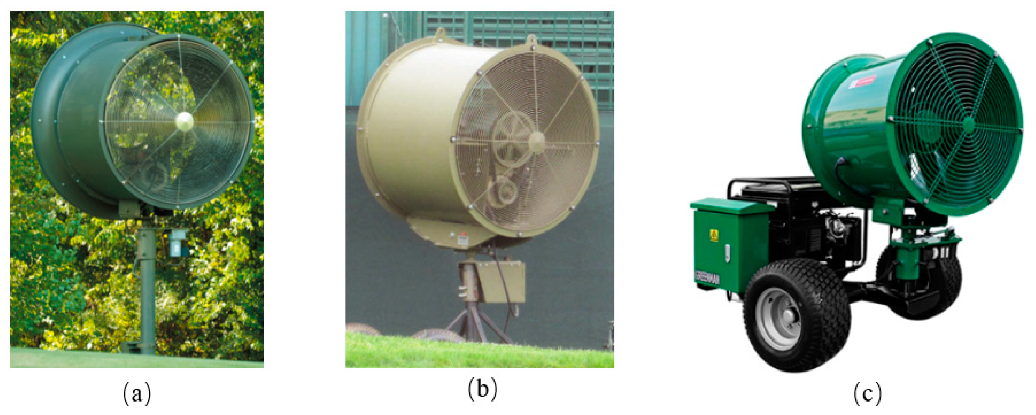
:1. Introduction
2. Materials and Methods
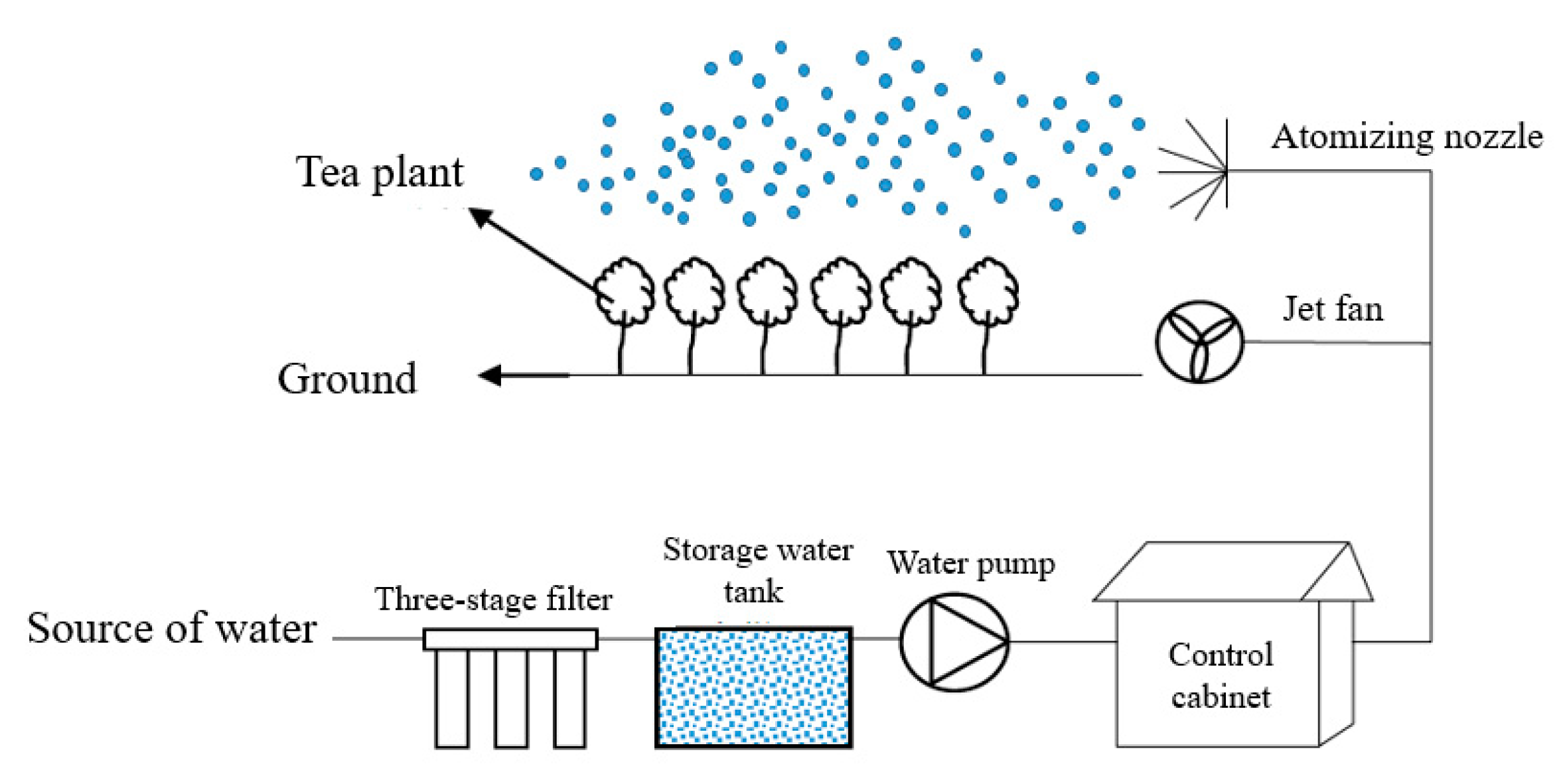
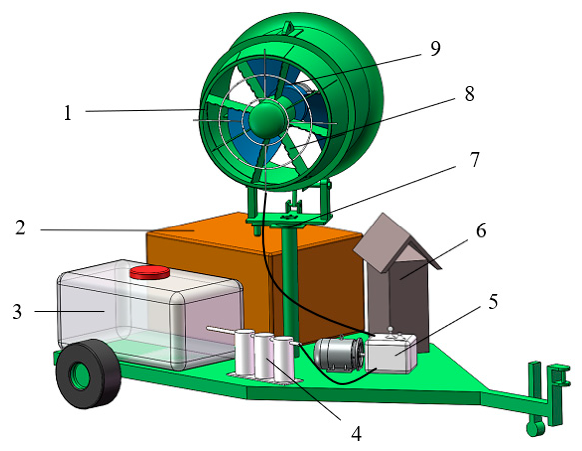
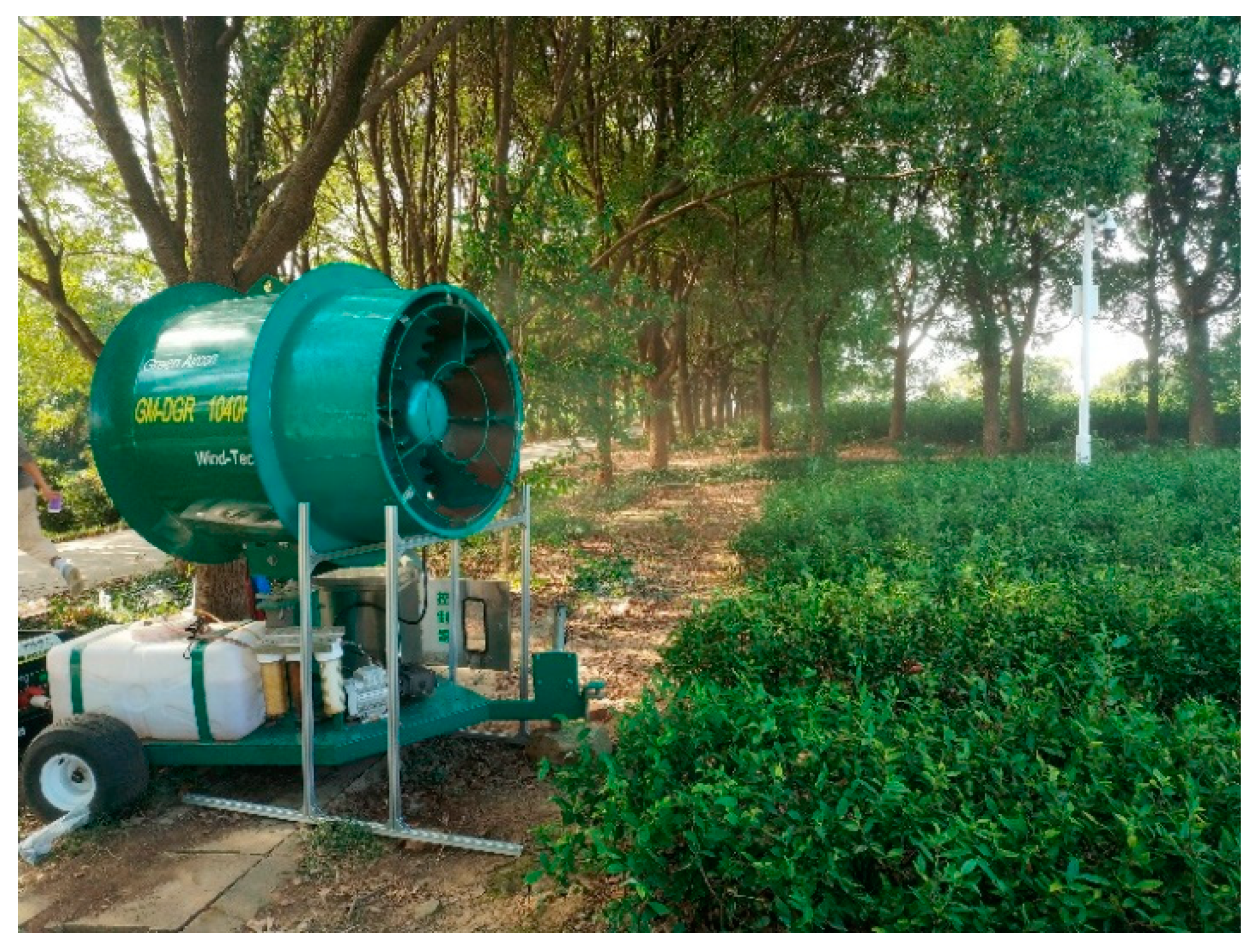
2.1. General Composition and Working Principle of Spray Cooling Fan
2.2. Structure Design of Air Duct
2.3. Key Parameter Optimization of Air Duct Based on CFD Simulation
2.3.1. Basic Governing Equation
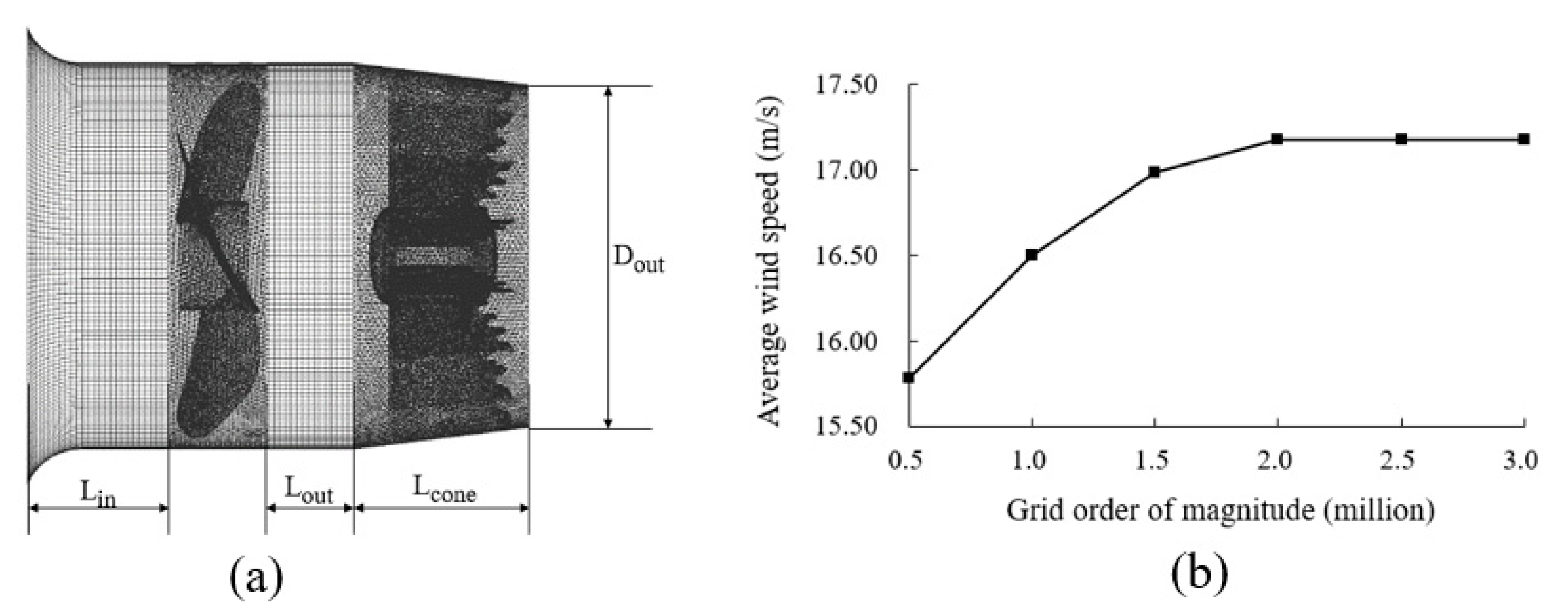
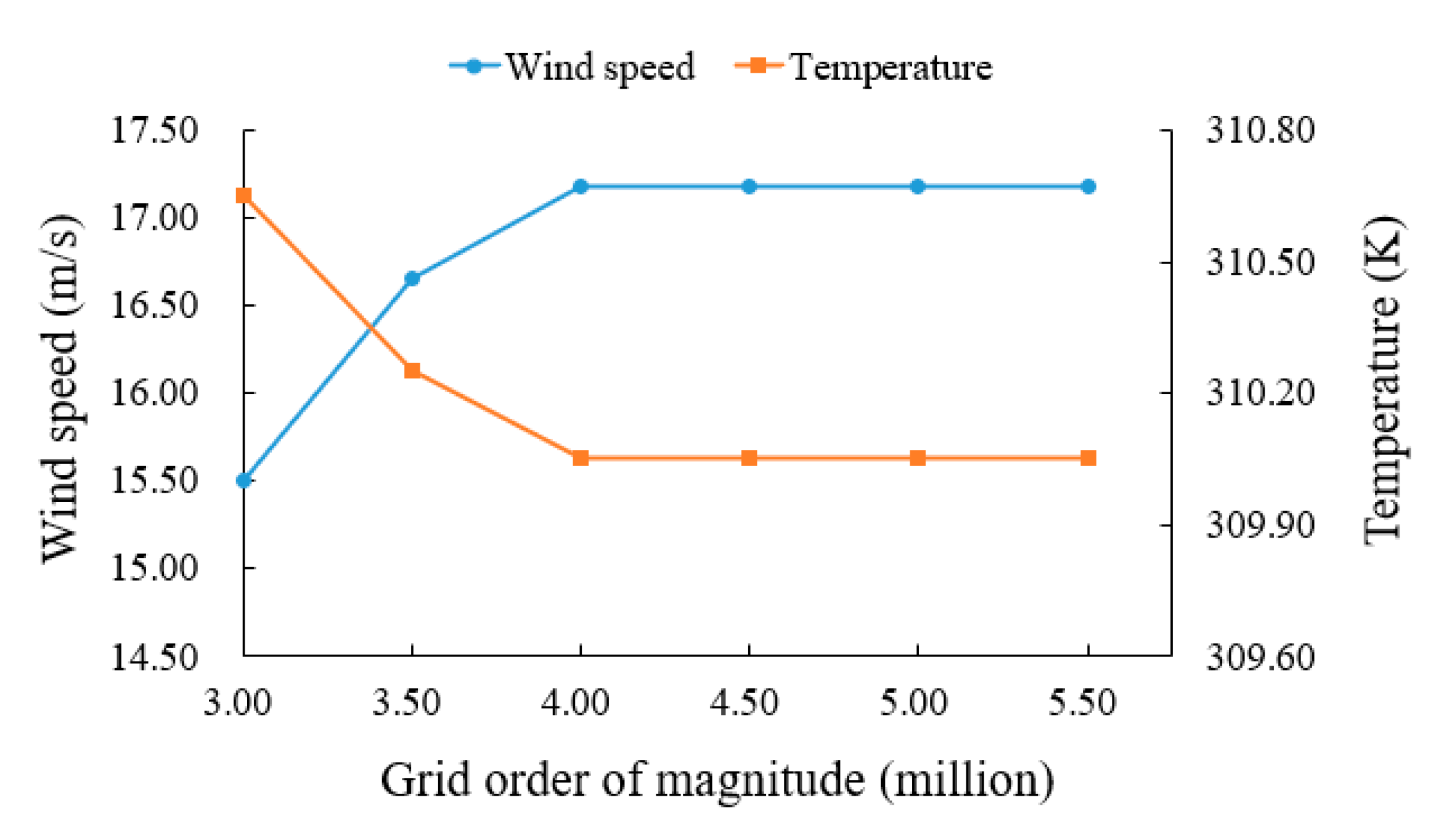
2.3.2. Meshing and Computing Method
2.3.3. Performance Indicator of Jet Fan
2.3.4. RSM Experimental Design
2.4. Optimization of Spray Parameters Based on Multiphase Flow Simulation
2.4.1. Construction of Mathematical Model
Species Transport Model
Discrete Phase Model
Porous Media Model
Radiation Model
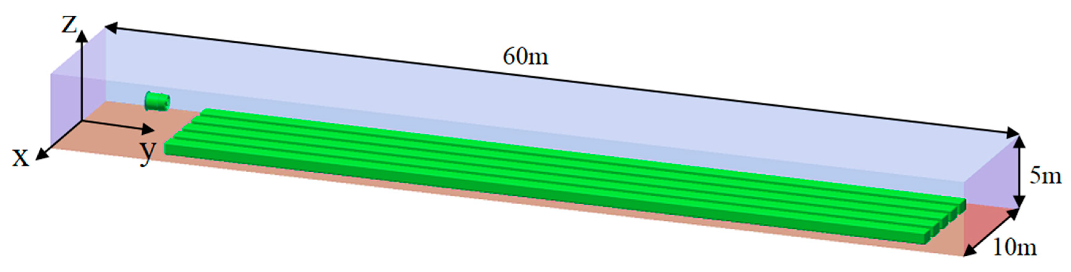
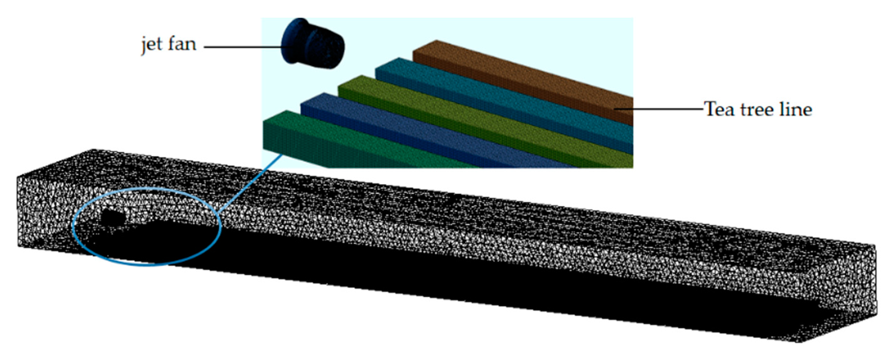
2.4.2. Physical Model and Mesh Generation
2.4.3. Boundary Conditions and Calculation Settings
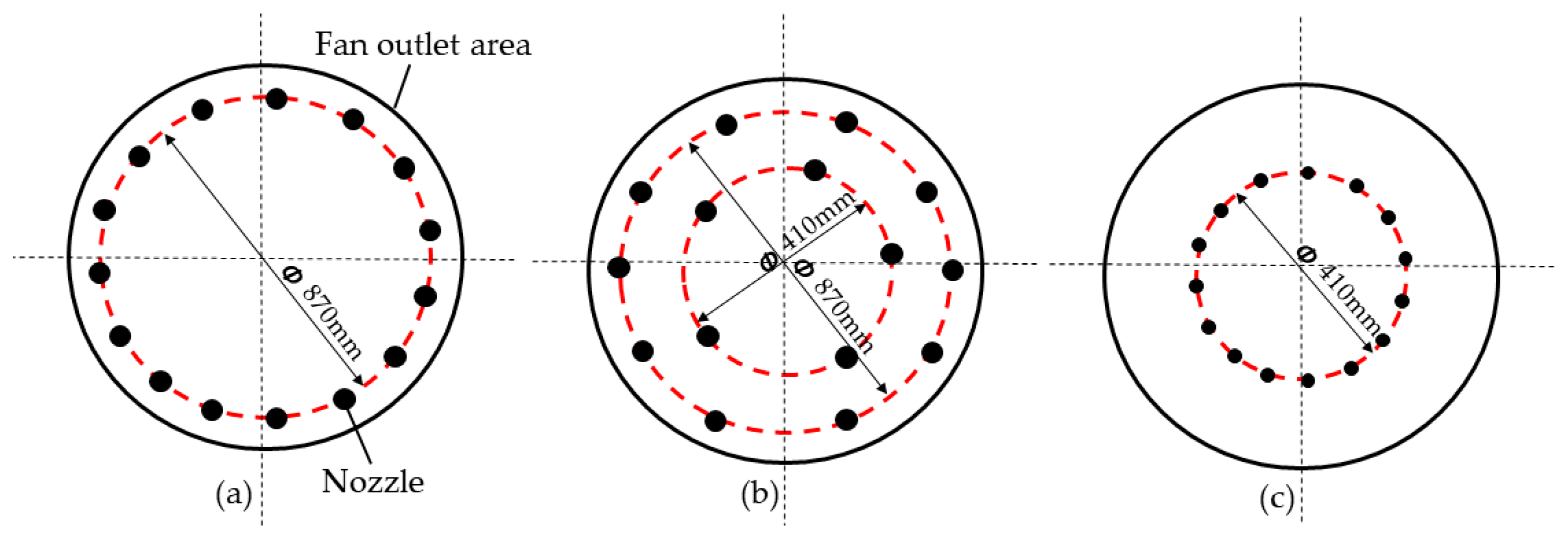
2.4.4. Orthogonal Experimental Design
2.5. Field Test of Spray Cooling Fan
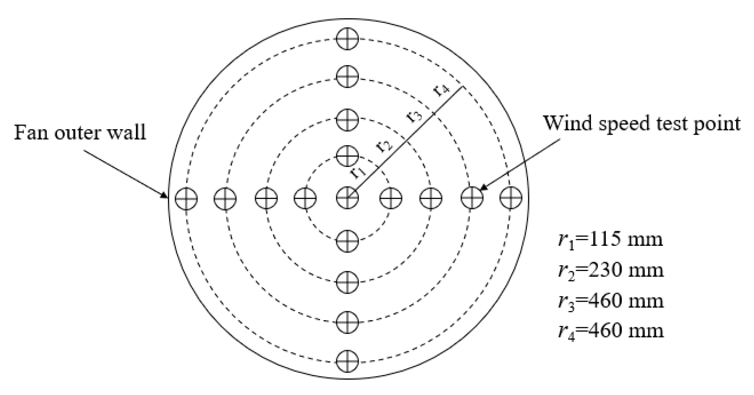
2.5.1. Performance Test of Jet Fan
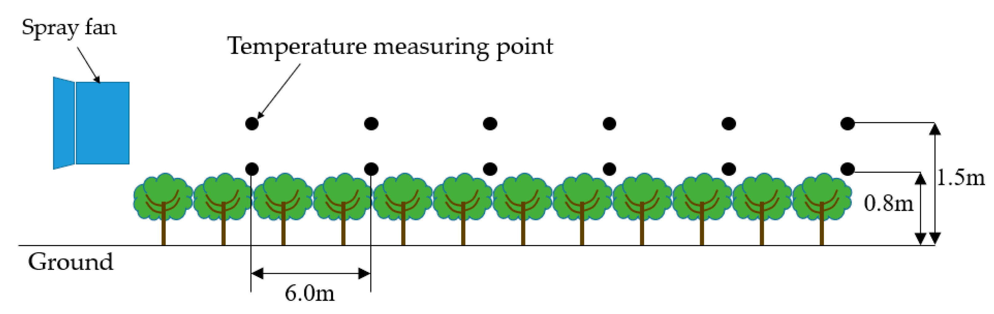
2.5.2. Effect of Spray Cooling on Tea Fields
- The spray cooling system was moved to the front end of the tea tree row, and the center line of the jet fan was 1.5 m high above ground.
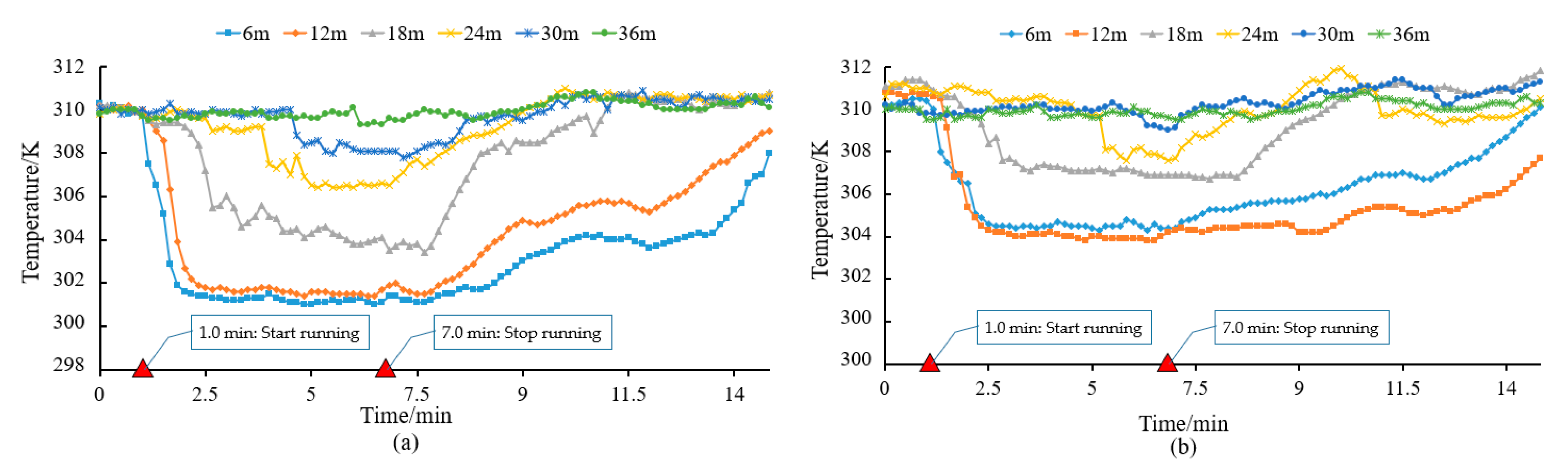
- The temperature recorders were initiated 10 min before testing the temperature distribution of the tea field.
- In the period of high temperature without wind, the jet fan and atomization system were initiated at the same time, the pressure of the high-pressure plunger pump was set to 5 MPa.
- According to the preliminary test results, the continuous operation time was set to 6.0 min to ensure the stability of air temperature.
- After the system closed, the temperature recorder was collected for data analysis.
3. Results and Discussion
3.1. Simulation Results and Analysis of Airflow Field in Air Duct
3.1.1. Results of RSM Experiment
3.1.2. Variance Analysis
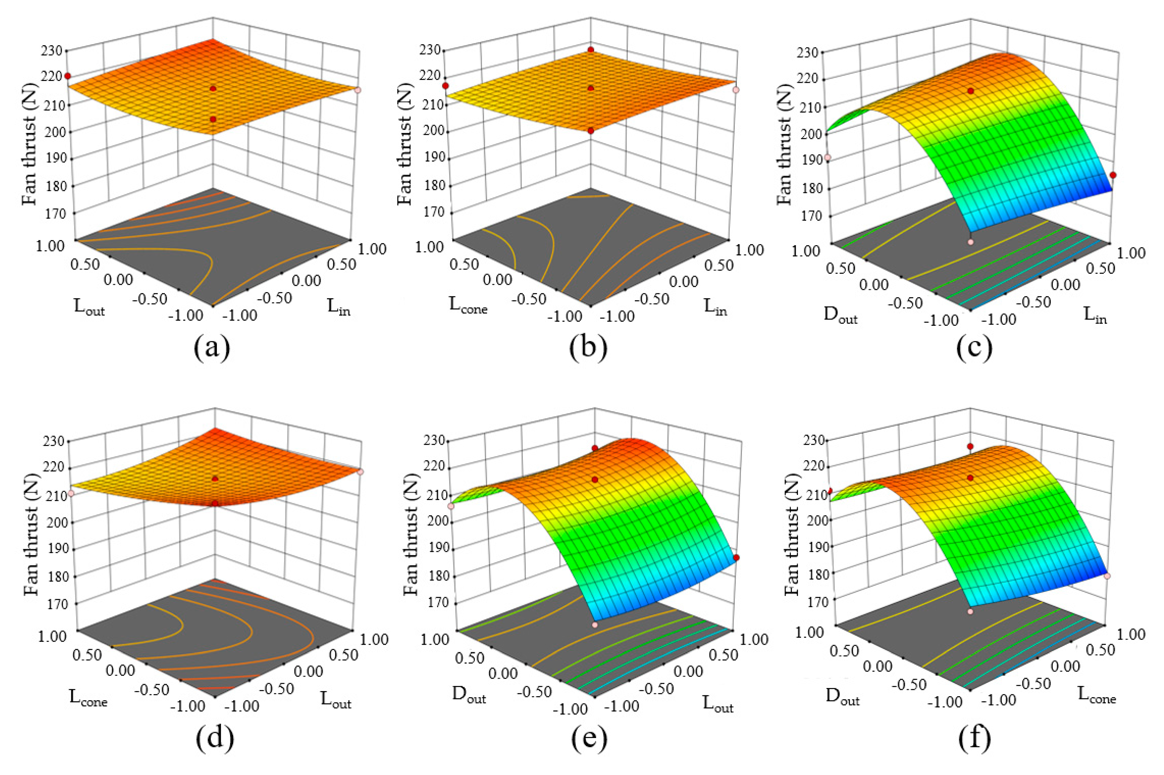
3.1.3. Analysis of Interaction between Two Factors
3.1.4. Simulation Results of Optimized Parameters
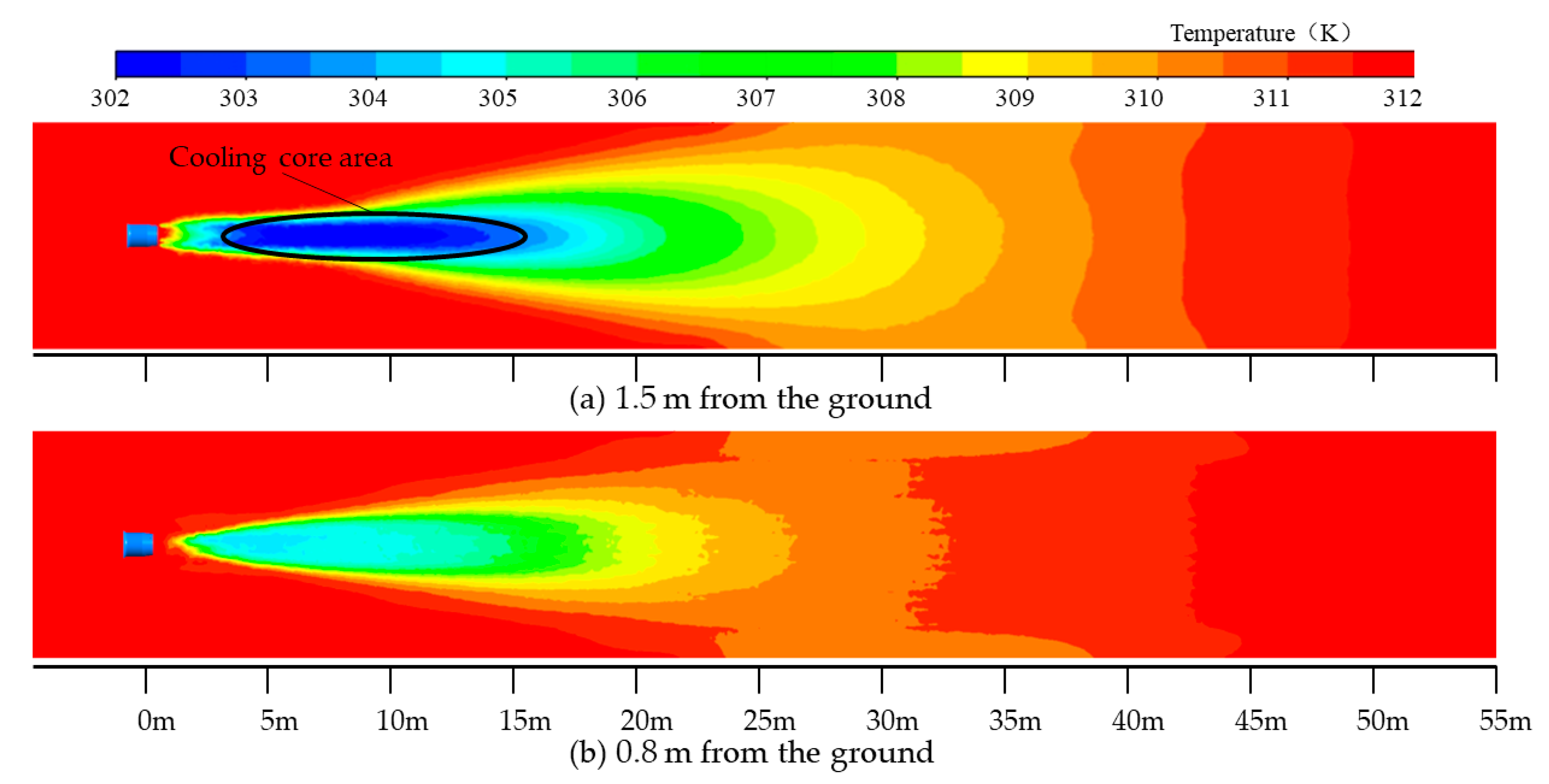
3.2. Simulation and Analysis of Spray Cooling for Multiphase Flow
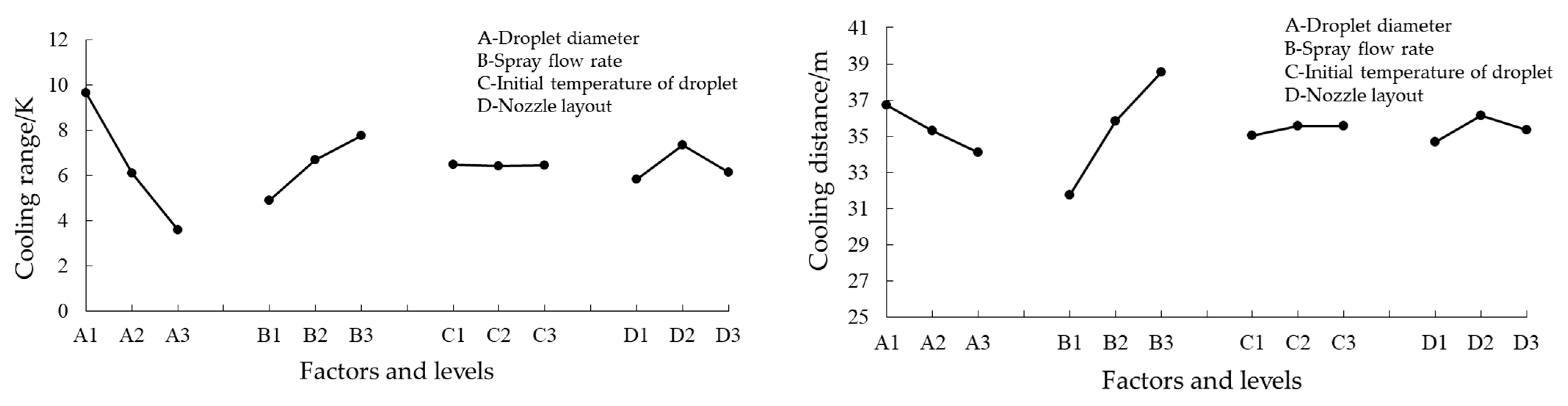
- For the maximum temperature drop: A1B3C1D2;
- For the effective distance of cooling: A1B3C2or3D2.
3.3. Field Test Results and Analysis
3.3.1. Performance Test Results Analysis of Jet Fan
3.3.2. Test Result Analysis of Cooling Effect of Spray Cooling Fan
4. Conclusions
Author Contributions
Funding
Institutional Review Board Statement
Informed Consent Statement
Data Availability Statement
Conflicts of Interest
References
- Ren, T.; Zheng, P.; Zhang, K.; Liao, J.; Xiong, F.; Shen, Q.; Ma, Y.; Fang, W.; Zhu, X. Effects of GABA on the polyphenol accumulation and antioxidant activities in tea plants (Camellia sinensis L.) under heat-stress conditions. Plant Physiol. Biochem. 2021, 159, 363–371. [Google Scholar] [CrossRef] [PubMed]
- Webb, L.; Darbyshire, R.; Goodwin, I. Climate Change: Horticulture. In Encyclopedia of Agriculture and Food Systems; Van Alfen, N.K., Ed.; Academic Press: Oxford, UK, 2014; pp. 266–283. [Google Scholar]
- Ahmed, H.A.; Tong, Y.-X.; Yang, Q.-C.; Al-Faraj, A.A.; Abdel-Ghany, A.M. Spatial distribution of air temperature and relative humidity in the greenhouse as affected by external shading in arid climates. J. Integr. Agric. 2019, 18, 2869–2882. [Google Scholar] [CrossRef]
- García, M.L.; Medrano, E.; Sánchez-Guerrero, M.C.; Lorenzo, P. Climatic effects of two cooling systems in greenhouses in the Mediterranean area: External mobile shading and fog system. Biosyst. Eng. 2011, 108, 133–143. [Google Scholar] [CrossRef]
- Gao, Y.; Shao, S.; Tian, S.; Xu, H.; Tian, C. Energy consumption analysis of the forced-air cooling process with alternating ventilation mode for fresh horticultural produce. Energy Procedia 2017, 142, 2642–2647. [Google Scholar] [CrossRef]
- Ulpiani, G. Water mist spray for outdoor cooling: A systematic review of technologies, methods and impacts. Appl. Energy 2019, 254, 113647. [Google Scholar] [CrossRef]
- Tai, C.; Sawada, Y.; Masuda, J.; Daimon, H.; Fukao, Y. Cultivation of spinach in hot seasons using a micro-mist-based temperature-control system. Sci. Hortic. 2020, 273, 109603. [Google Scholar] [CrossRef]
- Almuhanna, E.A.; Gamea, G.R.; Osman, O.E.; Almahdi, F.M. Performance of roof-mounted misting fans to regulate heat stress in dairy cows. J. Therm. Biol. 2021, 99, 102984. [Google Scholar] [CrossRef]
- Sethi, V.P.; Sharma, S.K. Survey of cooling technologies for worldwide agricultural greenhouse applications. Sol. Energy 2007, 81, 1447–1459. [Google Scholar] [CrossRef]
- Saberian, A.; Sajadiye, S.M. Assessing the variable performance of fan-and-pad cooling in a subtropical desert greenhouse. Appl. Therm. Eng. 2020, 179, 115672. [Google Scholar] [CrossRef]
- López, A.; Valera, D.L.; Molina-Aiz, F.D.; Peña, A. Sonic anemometry to evaluate airflow characteristics and temperature distribution in empty Mediterranean greenhouses equipped with pad–fan and fog systems. Biosyst. Eng. 2012, 113, 334–350. [Google Scholar] [CrossRef]
- Banik, P.; Ganguly, A. Performance and economic analysis of a floricultural greenhouse with distributed fan-pad evaporative cooling coupled with solar desiccation. Sol. Energy 2017, 147, 439–447. [Google Scholar] [CrossRef]
- Çaylı, A.; Akyüz, A.; Üstün, S.; Yeter, B. Efficiency of two different types of evaporative cooling systems in broiler houses in Eastern Mediterranean climate conditions. Therm. Sci. Eng. Prog. 2021, 22, 100844. [Google Scholar] [CrossRef]
- Farnham, C.; Nakao, M.; Nishioka, M.; Nabeshima, M.; Mizuno, T. Study of mist-cooling for semi-enclosed spaces in Osaka, Japan. Procedia Environ. Sci. 2011, 4, 228–238. [Google Scholar] [CrossRef] [Green Version]
- Zhu, L.; Xue, X.; Jia, W.; Ding, S.; Sun, Z. Application of CFD technology in air-assisted spraying in orchard and analysis of its prospects. J. Drain. Irrig. Mach. Eng. 2014, 32, 776–782. [Google Scholar]
- Brandl, D.; Mach, T.; Heimrath, R.; Edtmayer, H.; Hochenauer, C. Thermal evaluation of a component heating system for a monastery cell with measurements and CFD simulations. J. Build. Eng. 2021, 39, 102264. [Google Scholar] [CrossRef]
- de Almeida Leão, R.X.; Silva Amorim, L.; Ferreira Martins, M.; Belich Junior, H.; Sarcinelli, E.; Amarante Mesquita, A.L. Airborne flow dynamics near free-falling bulk materials: CFD analysis from analytical pressure field. Powder Technol. 2021, 385, 1–11. [Google Scholar] [CrossRef]
- Negi, P.; Subhash, M. Method to control flow separation over wind turbine blade: A CFD study. Mater. Today Proc. 2021. [Google Scholar] [CrossRef]
- Sureshkumar, R.; Kale, S.R.; Dhar, P.L. Heat and mass transfer processes between a water spray and ambient air—II. Simulations. Appl. Therm. Eng. 2008, 28, 361–371. [Google Scholar] [CrossRef]
- Sureshkumar, R.; Kale, S.R.; Dhar, P.L. Heat and mass transfer processes between a water spray and ambient air—I. Experimental data. Appl. Therm. Eng. 2008, 28, 349–360. [Google Scholar] [CrossRef]
- Zhang, W.; Yuan, J.; Zhou, B.; Li, H.; Yuan, Y. The influence of axial-flow fan trailing edge structure on internal flow. Adv. Mech. Eng. 2018, 10(11), 168781401881174. [Google Scholar] [CrossRef] [Green Version]
- Söylemez, E.; Alpman, E.; Onat, A.; Hartomacıoğlu, S. CFD analysis for predicting cooling time of a domestic refrigerator with thermoelectric cooling system. Int. J. Refrig. 2021, 123, 138–149. [Google Scholar] [CrossRef]
- Zhang, X.; Weerasuriya, A.U.; Tse, K.T. CFD simulation of natural ventilation of a generic building in various incident wind directions: Comparison of turbulence modelling, evaluation methods, and ventilation mechanisms. Energy Build. 2020, 229, 110516. [Google Scholar] [CrossRef]
- Khan, S.A.; Ibrahim, O.M.; Aabid, A. CFD analysis of compressible flows in a convergent-divergent nozzle. Mater. Today Proc. 2021. [Google Scholar] [CrossRef]
- Xie, B.; Xiao, F. Toward efficient and accurate interface capturing on arbitrary hybrid unstructured grids: The THINC method with quadratic surface representation and Gaussian quadrature. J. Comput. Phys. 2017, 349, 415–440. [Google Scholar] [CrossRef]
- Gullberg, P.; Löfdahl, L. Fan modelling in CFD using RANS with MRF, limitations and consistency, a comparison between fans of different design. In Vehicle Thermal Management Systems Conference and Exhibition (VTMS10); Woodhead Publishing: Cambridge, UK, 2011; pp. 423–433. [Google Scholar]
- Boulard, T.; Roy, J.C.; Lamrani, M.A.; Haxaire, R. Characterising and Modelling the Air Flow and Temperature Profiles in a Closed Greenhouse in Diurnal Conditions. IFAC Proc. Vol. 1997, 30, 37–42. [Google Scholar] [CrossRef]
- Liu, W.; Wang, J.B.; Liu, Z.C. A method of fluid dynamic analysis based on Navier-Stokes equation and conservation equation on fluid mechanical energy. Int. J. Heat Mass Transf. 2017, 109, 393–396. [Google Scholar] [CrossRef]
- Zhang, Y.C.; Yi, D.L.; Feng, D.Y. Fan Design and Selection; Chemical Industry Press: Beijing, China, 2011. [Google Scholar]
- Ye, W.; Wang, X.; Liu, Y.; Chen, J. Analysis and prediction of the performance of free- piston Stirling engine using response surface methodology and artificial neural network. Appl. Therm. Eng. 2021, 188, 116557. [Google Scholar] [CrossRef]
- Breig, S.J.M.; Luti, K.J.K. Response surface methodology: A review on its applications and challenges in microbial cultures. Mater. Today Proc. 2021. [Google Scholar] [CrossRef]
- Zhao, W.; Ma, A.; Ji, J.; Chen, X.; Yao, T. Multi-Objective Optimization of a Double-Side Linear Vernier PM Motor Using Response Surface Method and Differential Evolution. IEEE Trans. Ind. Electron. 2019, 99. [Google Scholar] [CrossRef]
- Murugan, P.C.; Joseph Sekhar, S. Species – Transport CFD model for the gasification of rice husk (Oryza Sativa) using downdraft gasifier. Comput. Electron. Agric. 2017, 139, 33–40. [Google Scholar] [CrossRef]
- Bing, X.; Sun, D.; Song, S.; Xue, X.; Dai, Q. Simulation and experimental research on droplet flow characteristics and deposition in airflow field. Int. J. Agric. Biol. Eng. 2020, 13, 16–24. [Google Scholar]
- Mahgoub, A.O.; Ghani, S. Numerical and experimental investigation of utilizing the porous media model for windbreaks CFD simulation. Sustain. Cities Soc. 2021, 65, 102648. [Google Scholar] [CrossRef]
- Saneinejad, S.; Moonen, P.; Defraeye, T.; Derome, D.; Carmeliet, J. Coupled CFD, radiation and porous media transport model for evaluating evaporative cooling in an urban environment. J. Wind Eng. Ind. Aerodyn. 2012, 104–106, 455–463. [Google Scholar] [CrossRef]
- Houcine, A.; Maatallah, T.; Alimi, S.E.; Nasrallah, S.B. Optical modeling and investigation of sun tracking parabolic trough solar collector basing on Ray Tracing 3Dimensions-4Rays. Sustain. Cities Soc. 2017, 35, 786–798. [Google Scholar] [CrossRef]
- Zhao, B.J.; Hou, D.H.; Chen, H.L.; Yu, W.; Qiu, J. Optimization design of a double-channel pump by means of orthogonal test, CFD, and experimental analysis. Adv. Mech. Eng. 2014, 6, 1–10. [Google Scholar] [CrossRef] [Green Version]


| Installation Angle (°) | Swept Angle (°) | Hub Ratio | Number of Leaves | Rotation Diameter (mm) |
|---|---|---|---|---|
| 18 | 86 | 0.29 | 3 | 1040 |
| Level | Factors | |||
|---|---|---|---|---|
| Lin (mm) | Lout (mm) | Lcone (mm) | Dout (mm) | |
| −1 | 100 | 100 | 200 | 800 |
| 0 | 250 | 250 | 350 | 900 |
| 1 | 400 | 400 | 500 | 1000 |
| Levels | Factors | |||
|---|---|---|---|---|
| Dd (μm) | Qm (kg/min) | Ti (K) | Nozzle Layout | |
| 1 | 15–45 | 2.5 | 288.15 | a |
| 2 | 45–75 | 3.5 | 298.15 | b |
| 3 | 75–105 | 4.5 | 308.15 | c |
| Experiment Number | Factors | Indicator | |||
|---|---|---|---|---|---|
| Lin | Lout | Lcone | Lout | Thrust (N) | |
| 1 | 0 | 0 | −1 | 1 | 211.81 |
| 2 | 0 | −1 | 0 | 1 | 206.88 |
| 3 | −1 | 0 | 0 | 1 | 192.37 |
| 4 | 0 | 0 | 0 | 0 | 216.49 |
| 5 | 0 | 1 | −1 | 0 | 219.32 |
| 6 | 0 | −1 | 1 | 0 | 224.21 |
| 7 | 0 | 0 | 1 | −1 | 179.21 |
| 8 | 0 | −1 | 0 | −1 | 184.51 |
| 9 | 0 | 0 | 1 | 1 | 214.48 |
| 10 | 1 | 1 | 0 | 0 | 219.64 |
| 11 | 0 | 0 | 0 | 0 | 216.49 |
| 12 | 0 | 0 | −1 | −1 | 187.38 |
| 13 | −1 | 0 | 1 | 0 | 217.69 |
| 14 | 0 | 1 | 1 | 0 | 217.71 |
| 15 | −1 | 0 | −1 | 0 | 218.54 |
| 16 | 0 | 0 | 0 | 0 | 216.49 |
| 17 | 0 | 1 | 0 | −1 | 187.78 |
| 18 | 0 | 0 | 0 | 0 | 216.49 |
| 19 | 1 | 0 | 0 | −1 | 185.76 |
| 20 | 0 | 0 | 0 | 0 | 216.49 |
| 21 | 1 | 0 | −1 | 0 | 216.20 |
| 22 | −1 | −1 | 0 | 0 | 222.21 |
| 23 | 0 | −1 | 1 | 0 | 211.55 |
| 24 | 1 | −1 | 0 | 0 | 216.15 |
| 25 | 1 | 0 | 0 | 1 | 211.97 |
| 26 | −1 | 1 | 0 | 0 | 221.19 |
| 27 | 0 | 1 | 0 | 1 | 214.11 |
| 28 | 1 | 0 | 1 | 0 | 217.23 |
| 29 | −1 | 0 | 0 | −1 | 183.07 |
| Source | Sum of Squares | df | Mean Square | F-Value | p-Value | |
|---|---|---|---|---|---|---|
| Model | 5160.12 | 14 | 368.58 | 18.09 | <0.0001 | significant |
| A | 11.76 | 1 | 11.76 | 0.5773 | 0.4600 | |
| B | 16.90 | 1 | 16.90 | 0.8295 | 0.3778 | |
| C | 31.98 | 1 | 31.98 | 1.57 | 0.2308 | |
| D | 1725.84 | 1 | 1725.84 | 84.71 | <0.0001 | |
| AB | 5.09 | 1 | 5.09 | 0.2496 | 0.6251 | |
| AC | 0.8836 | 1 | 0.8836 | 0.0434 | 0.8380 | |
| AD | 71.49 | 1 | 71.49 | 3.51 | 0.0821 | |
| BC | 30.53 | 1 | 30.53 | 1.50 | 0.2411 | |
| BD | 3.92 | 1 | 3.92 | 0.1924 | 0.6676 | |
| CD | 29.38 | 1 | 29.38 | 1.44 | 0.2497 | |
| A2 | 1.84 | 1 | 1.84 | 0.0904 | 0.7681 | |
| B2 | 36.50 | 1 | 36.50 | 1.79 | 0.2021 | |
| C2 | 8.29 | 1 | 8.29 | 0.4072 | 0.5337 | |
| D2 | 2825.01 | 1 | 2825.01 | 138.67 | <0.0001 | |
| Residual | 285.22 | 14 | 20.37 | |||
| Lack of Fit | 285.22 | 10 | 28.52 | |||
| Pure Error | 0.0000 | 4 | 0.0000 | |||
| Cor Total | 5445.33 | 28 |
| Thrust (N) | Average Speed (m/s) | |
|---|---|---|
| Optimize predicted value | 229.12 | 17.18 |
| Simulation value | 225.06 | 17.02 |
| Relative error (%) | 1.8 | 3.9 |
| Testing Order Number | Factors | Indicators | |||||
|---|---|---|---|---|---|---|---|
| A | B | C | D | Temperature Drop | Effective Distance of Cooling | ||
| 1 | 1 | 1 | 1 | 1 | 7.5 | 32.01 | |
| 2 | 1 | 2 | 2 | 2 | 10.72 | 38.12 | |
| 3 | 1 | 3 | 3 | 3 | 10.67 | 40.06 | |
| 4 | 2 | 1 | 2 | 3 | 4.18 | 31.81 | |
| 5 | 2 | 2 | 3 | 1 | 5.71 | 35.23 | |
| 6 | 2 | 3 | 1 | 2 | 8.34 | 38.85 | |
| 7 | 3 | 1 | 3 | 2 | 2.93 | 31.40 | |
| 8 | 3 | 2 | 1 | 3 | 3.58 | 34.21 | |
| 9 | 3 | 3 | 2 | 1 | 4.26 | 36.75 | |
| Temperature drop | K1 | 28.89 | 14.61 | 19.42 | 17.47 | ||
| K2 | 18.23 | 20.01 | 19.16 | 21.99 | |||
| K3 | 10.77 | 23.27 | 19.31 | 18.43 | |||
| k1 | 9.63 | 4.87 | 6.47 | 5.82 | |||
| k2 | 6.08 | 6.67 | 6.39 | 7.33 | |||
| k3 | 3.59 | 7.76 | 6.44 | 6.14 | |||
| Range | 6.04 | 2.89 | 0.08 | 1.51 | |||
| Primary and secondary factors | ABDC | ||||||
| Optimal solution | A1B3C1D2 | ||||||
| Effective distance of cooling | K1 | 110.19 | 95.22 | 105.07 | 103.99 | ||
| K2 | 105.89 | 107.56 | 106.68 | 108.37 | |||
| K3 | 102.36 | 115.66 | 106.69 | 106.08 | |||
| k1 | 36.73 | 31.74 | 35.02 | 34.66 | |||
| k2 | 35.30 | 35.85 | 35.56 | 36.12 | |||
| k3 | 34.12 | 38.55 | 35.56 | 35.36 | |||
| Range | 2.61 | 6.81 | 0.54 | 1.46 | |||
| Primary and secondary factors | BADC | ||||||
| Optimal solution | A1B3C2or3D2 | ||||||
| Wind Speed (m/s) | Thrust (N) | |
|---|---|---|
| Simulation value | 17.02 | 225.06 |
| Test value | 17.25 | 231.52 |
| Relative error (%) | 2.9 | 2.8 |
| Vertical Height | Simulation and Experimental Results (K) | Distance from Fan | |||||
|---|---|---|---|---|---|---|---|
| 6 m | 12 m | 18 m | 24 m | 30 m | 36 m | ||
| 1.5 m | Simulation results | 10.1 | 10.0 | 7.2 | 4.3 | 3.2 | 1.8 |
| Test result | 9.1 | 8.7 | 6.3 | 4.1 | 2.1 | 1.1 | |
| Error | 1.0 | 1.3 | 0.9 | 0.2 | 1.1 | 0.7 | |
| 0.8 m | Simulation results | 7.1 | 6.9 | 6.1 | 2.1 | 1.5 | 0.8 |
| Test result | 6.5 | 7.1 | 5.2 | 2.8 | 0.8 | 0.6 | |
| Error | 0.6 | 0.2 | 0.9 | 0.7 | 0.7 | 0.2 | |
Publisher’s Note: MDPI stays neutral with regard to jurisdictional claims in published maps and institutional affiliations. |
© 2021 by the authors. Licensee MDPI, Basel, Switzerland. This article is an open access article distributed under the terms and conditions of the Creative Commons Attribution (CC BY) license (https://creativecommons.org/licenses/by/4.0/).
Share and Cite
Hu, Y.; Chen, Y.; Wei, W.; Hu, Z.; Li, P. Optimization Design of Spray Cooling Fan Based on CFD Simulation and Field Experiment for Horticultural Crops. Agriculture 2021, 11, 566. https://doi.org/10.3390/agriculture11060566
Hu Y, Chen Y, Wei W, Hu Z, Li P. Optimization Design of Spray Cooling Fan Based on CFD Simulation and Field Experiment for Horticultural Crops. Agriculture. 2021; 11(6):566. https://doi.org/10.3390/agriculture11060566
Chicago/Turabian StyleHu, Yongguang, Yongkang Chen, Wuzhe Wei, Zhiyuan Hu, and Pingping Li. 2021. "Optimization Design of Spray Cooling Fan Based on CFD Simulation and Field Experiment for Horticultural Crops" Agriculture 11, no. 6: 566. https://doi.org/10.3390/agriculture11060566