Currents Status, Challenges, and Future Directions in Identifying Critical Source Areas for Non-Point Source Pollution in Canadian Conditions


 , ,
, , 
Abstract
:1. Introduction
2. Methods to Determine CSAs
2.1. Simple Methods
2.1.1. Phosphorus Index (PI)
2.1.2. Topographic Index (TI)
2.1.3. Other Miscellaneous Methods
2.2. Detailed HWQ Models for CSAs
3. Current State and Challenges of Determining CSAs
3.1. Level of Model Complexity and Scaling Issues
3.2. Representation of Phosphorus Transformation and Transport Processes
3.3. Landscape Connectivity to Stream System Accounted for
3.4. Modeling Practices
3.5. Canadian Hydrological Conditions Conceptualization in Models
3.5.1. Runoff Generation Mechanism
3.5.2. Landscape Depressions
3.5.3. Cold-Climate Conditions
3.5.4. Tile Drains
4. Future Research Directions
- A better database is needed to improve the model prediction capability. More importantly, the TI method will benefit from better resolution data, such as Light Detection and Ranging (LiDAR) data, which could also be helpful to incorporate the saturation excess runoff generation into HWQ models.
- Most BMPs are implemented at the field scale. Therefore, it is important to improve field or sub-field scale modeling capability of the existing methods. This is particularly important while using semi-distributed HWQ models such as SWAT. This can be achieved by developing an ArcGIS extension that can identify an HRU location within a sub-basin. This will also facilitate evaluation of field and sub-field level output.
- There also is a need for improvements in the predictions of dissolved P in surface runoff from soil, which is now typically based on simple extraction coefficients relating a measure of soil P (usually routine soil tests) to dissolved P concentrations in runoff. Most existing methods use a constant value for all soil types. It is, therefore, necessary to conduct research to identify the variations in extraction coefficients with soil properties such as soil texture.
- With significant variations at field and watershed scale estimation of P loss, it is important to further investigate if different algorithms for sediment and P loss should be used.
- Canadian hydrology exhibits a distinct seasonal pattern. It is, therefore, necessary to quantify and include the impact of seasonal hydrology of P generation and transport processes in HWQ modeling approaches.
- With better understanding of physical, chemical, and biological processes affecting water quality, future research should also focus on improving the representation of processes, such as P stratification and legacy sources in HWQ models. Both vertical stratifications of P in no-till soils and legacy sources of P need to be incorporated as they affect the short-term benefits of remedial practices applied to CSAs.
- Another research area that needs attention is nutrient processes in the wetland modules. For example, the ‘Wetland’ and ‘Pond’ modules of the SWAT model do not consider nutrient transformation. However, several field studies have indicated that transformation of nutrients indeed occurs within the ponds, wetlands, or potholes.
- Development of a ‘Toolbox’ to identify CSAs also needs serious attention and could be a step forward. In fact, Sharpley et al. [28] envisioned the need and value of such a ‘Toolbox’. Especially given the fact that it is very difficult to answer all pertaining questions related to identifying CSAs of NPS pollution using a single model/method. The envisioned ‘Toolbox’ can host a range of different models/methods, ranging from a simple method such as topographic index to a complex HWQ model. This will provide the end users with a variety of options to try to use different methods/models to identify CSAs. Users may opt to use the simple methods for screening larger watersheds while detailed HWQ models may be used to provide absolute values of P loss and long-term effects of future management scenarios on P loss. The ‘Toolbox’ can be hosted in a dedicated platform or can be made available as a web-based modeling framework such as the Hydrology and Water Quality System (HAWQS) using SWAT framework [202]. The ‘Toolbox’ essentially offers features such as an automated workflow of input data preparing and processing for an area of user’s choice and output data repository to store model and scenario runs. We believe that provision of such a ‘Toolbox’ renders the redundancies associated with pre-processing of large volume of input data (e.g., spatial and meteorological) which is often time-intensive and error-prone. Recent advances in computing facilities and web technologies also support the idea of making the envisioned ‘Toolbox’ available to the wider public.
- With advances in computational resources and techniques, future research on CSAs should focus on the sources of uncertainty, uncertainty quantification methods, and incorporation of all possible uncertainties in HWQ modeling approaches.
- With advances in instrumentation technology, future research should also focus on field research to identify CSAs. Special attention is needed on the quantification on the seasonal variability of CSAs. Data collected from such experiments will be useful to evaluate the CSA prediction capability of HWQ models.
- It has been shown that the majority of NPS pollution would be exported in the late winter and early spring months [31,171,203] and, therefore, constitute hot-moments of NPS pollution export. Sampling campaigns should be effective enough to capture the variability in such important time/seasons. Identification of the proper locations for water quality monitoring is equally important too. Thus, a cost-effective and efficient water quality monitoring framework, as suggested by Alilou et al. [204] is desired. Moreover, detailed HWQ model ideally needs continuous water quality data for proper calibration (and/or validation). However, such data are rarely available because of logistic issues. Often, sporadic water quality measurements are available which hinders proper model calibration (and/or validation) and model results may deem to be unreliable. This is a general problem in NPS pollution modeling. One possible solution is to carryout dedicated sampling campaigns to cover wide range of streamflow/field conditions (e.g., dry, wet, 24 h, etc.) which helps to verify a model’s ability in respective conditions [205]. However, this requires a team of dedicated crew waiting for such an event to occur, which may not always be available [206]. Another possibility is to install automatic samplers to measure some explanatory variables (e.g., specific conductance, turbidity) and using an established relationship (e.g., regression model), other water quality variables (e.g., total suspended solids, total phosphorus) are predicted [207]. However, uncertainties associate with such estimations render their use in calibrating (and/or validating) detailed HWQ models. The use of remote sensing technologies in validating HWQ model based CSAs can also be an alternative as shown by Shrestha et al. (in press). In the study, they used oblique aerial images to qualitatively validate CSA of phosphorus in a watershed. Such a technique may be useful for a large watershed, which needs water quality monitoring at multiple locations.
5. Conclusions
Author Contributions
Funding
Acknowledgments
Conflicts of Interest
References
- Peters, N.E.; Meybeck, M. Water Quality Degradation Effects on Freshwater Availability: Impacts of Human Activities. Water Int. 2000, 25, 185–193. [Google Scholar] [CrossRef]
- Hanjra, M.A.; Qureshi, M.E. Global water crisis and future food security in an era of climate change. Food Policy 2010, 35, 365–377. [Google Scholar] [CrossRef]
- United Nations. Water for Life Decade: Water Quality. 2016. Available online: http://www.un.org/waterforlifedecade/quality.shtml (accessed on 25 October 2016).
- Mitchell, M.J.; Driscoll, C.T.; Kahl, J.S.; Murdoch, A.P.S.; Pardo, L.H. Climatic Control of Nitrate Loss from Forested Watersheds in the Northeast United States. Environ. Sci. Technol. 1996, 30, 2609–2612. [Google Scholar] [CrossRef]
- Han, C.-W.; Xu, S.; Liu, J.; Lian, J.-J. Nonpoint-source nitrogen and phosphorus behavior and modeling in cold climate: A review. Water Sci. Technol. 2010, 62, 2277–2285. [Google Scholar] [CrossRef] [PubMed]
- Shrestha, N.K.; Wang, J. Water Quality Management of a Cold Climate Region Watershed in Changing Climate. J. Environ. Inform. 2019. [Google Scholar] [CrossRef]
- McConkey, B.; Nicholaichuk, W.; Steppuhn, H.; Reimer, C.D. Sediment yield and seasonal soil erodibility for semiarid cropland in western Canada. Can. J. Soil Sci. 1997, 77, 33–40. [Google Scholar] [CrossRef] [Green Version]
- Callesen, I.; Borken, W.; Kalbitz, K.; Matzner, E. Long-term development of nitrogen fluxes in a coniferous ecosystem: Does soil freezing trigger nitrate leaching? J. Plant Nutr. Soil Sci. 2007, 170, 189–196. [Google Scholar] [CrossRef]
- Dinar, A.; Seidl, P.; Olem, H.; Jorden, V.; Duda, A.; Johnson, R. Restoring and Protecting the World’s Lakes and Reservoirs; The World Bank: Washington, DC, USA, 1995; p. 155. [Google Scholar]
- Hanrahan, G.; Gardolinski, P.; Gledhill, M.; Worsfold, P. Environmental monitoring of nutrients. In Environmental Monitoring Handbook; Burden, F.R., Donnert, D., Goodish, T., McKelvie, I., Eds.; McGraw-Hill: New York, NY, USA, 2004; pp. 8.1–8.16. [Google Scholar]
- Brown, T.; Simpson, J. Managing phosphorus inputs to urban lakes: I. Determining the trophic state of your lake. Watershed Prot. Tech. 2001, 3, 771–781. [Google Scholar]
- Jørgensen, S.E.; Williams, W.D.; Centre, U.I.E.T.; International Lake Environment, C. Water Quality: The Impact of Eutrophication; UNEP-International Environment Technology Centre, International Lake Environment Committee Foundation: Kusatsu, Japan, 2001. [Google Scholar]
- Michalak, A.M.; Anderson, E.J.; Beletsky, D.; Boland, S.; Bosch, N.S.; Bridgeman, T.B.; Chaffin, J.D.; Cho, K.; Confesor, R.; Daloğlu, I.; et al. Record-setting algal bloom in Lake Erie caused by agricultural and meteorological trends consistent with expected future conditions. Proc. Natl. Acad. Sci. USA 2013, 110, 6448–6452. [Google Scholar] [CrossRef] [Green Version]
- Davis, C.C. Evidence for the Eutrophication of Lake Erie from Phytoplankton Records. Limnol. Oceanogr. 1964, 9, 275–283. [Google Scholar] [CrossRef]
- Makarewicz, J.C. Phytoplankton Biomass and Species Composition in Lake Erie, 1970 to 1987. J. Great Lakes Res. 1993, 19, 258–274. [Google Scholar] [CrossRef]
- Sweeney, R.A. Introduction: “Dead” sea of North America? Lake Erie in the 1960s and 70s. J. Great Lakes Res. 1993, 19, 198–199. [Google Scholar] [CrossRef]
- De Pinto, J.V.; Young, T.C.; McIlroy, L.M. Great lakes water quality improvement. Environ. Sci. Technol. 1986, 20, 752–759. [Google Scholar] [CrossRef] [PubMed]
- GLWQA. Great Lakes Water Quality Agreement. Available online: http://www.epa.gov/greatlakes/glwqa/1978/index.html (accessed on 25 August 2016).
- Lakes, G. Great Lakes Water Quality Agreement. Available online: http://ijc.org/files/tinymce/uploaded/GLWQA%202012.pdf (accessed on 25 August 2016).
- EPA. Recommended Phosphorus Loading Targets for Lake Erie. Available online: https://www.epa.gov/sites/production/files/2015-06/documents/report-recommended-phosphorus-loading-targets-lake-erie-201505.pdf (accessed on 13 January 2018).
- Sharpley, A.N.; Smith, S. Wheat tillage and water quality in the Southern plains. Soil Tillage Res. 1994, 30, 33–48. [Google Scholar] [CrossRef]
- Pieterse, N.; Bleuten, W.; Jørgensen, S. Contribution of point sources and diffuse sources to nitrogen and phosphorus loads in lowland river tributaries. J. Hydrol. 2003, 271, 213–225. [Google Scholar] [CrossRef]
- Van Bochove, E.; Thériault, G.; Dechmi, F.; Rousseau, A.; Quilbé, R.; Leclerc, M.-L.; Goussard, N. Indicator of risk of water contamination by phosphorus from Canadian agricultural land. Water Sci. Technol. 2006, 53, 303–310. [Google Scholar] [CrossRef] [PubMed]
- MOECC. Water Quality in Ontario 2014 Report. Available online: https://www.ontario.ca/page/water-quality-ontario-2014-report (accessed on 15 September 2016).
- Logan, T.J. Agricultural best management practices for water pollution control: Current issues. Agric. Ecosyst. Environ. 1993, 46, 223–231. [Google Scholar] [CrossRef]
- Parry, R. Agricultural Phosphorus and Water Quality: A U.S. Environmental Protection Agency Perspective. J. Environ. Qual. 1998, 27, 258–261. [Google Scholar] [CrossRef]
- D’Arcy, B.; Frost, A. The role of best management practices in alleviating water quality problems associated with diffuse pollution. Sci. Total. Environ. 2001, 265, 359–367. [Google Scholar] [CrossRef]
- Sharpley, A.N.; Kleinman, P.J.A.; Flaten, D.N.; Buda, A.R. Critical source area management of agricultural phosphorus: Experiences, challenges and opportunities. Water Sci. Technol. 2011, 64, 945–952. [Google Scholar] [CrossRef]
- Djodjic, F.; Spännar, M. Identification of critical source areas for erosion and phosphorus losses in small agricultural catchment in central Sweden. Acta Agric. Scand. Sect. B Plant Soil Sci. 2012, 62, 229–240. [Google Scholar] [CrossRef]
- Daggupati, P.; Douglas-Mankin, K.R.; Sheshukov, A.Y.; Barnes, P.L.; Devlin, D.L. Field-Level Targeting Using SWAT: Mapping Output from HRUs to Fields and Assessing Limitations of GIS Input Data. Trans. ASABE 2011, 54, 501–514. [Google Scholar] [CrossRef]
- Dickinson, W.T.; Rudra, R.; Wall, G.J. Identification of soil erosion and fluvial sediment problems. Hydrol. Process. 1986, 1, 111–1244. [Google Scholar] [CrossRef]
- Dickinson, W.T.; Rudra, R.P.; Sharma, D.N.; Singh, S.P. Employing a Watershed Model as a Basis for Planning A Sediment Monitoring Program. Can. Water Resour. J. 1994, 19, 289–303. [Google Scholar] [CrossRef]
- Pionke, H.B.; Gburek, W.J.; Sharpley, A.N.; Schnabel, R.R. Flow and nutrient export patterns for an agricultural hill-land watershed. Water Resour. Res. 1996, 32, 1795–1804. [Google Scholar] [CrossRef]
- Gburek, W.J.; Sharpley, A. Hydrologic Controls on Phosphorus Loss from Upland Agricultural Watersheds. J. Environ. Qual. 1998, 27, 267–277. [Google Scholar] [CrossRef]
- Yang, W.; Weersink, A. Cost-effective Targeting of Riparian Buffers. Can. J. Agric. Econ./Rev. Can. d’agroecon. 2004, 52, 17–34. [Google Scholar] [CrossRef]
- Sharpley, A.N.; Daniel, T.C.; Edwards, D.R. Phosphorus Movement in the Landscape. J. Prod. Agric. 1993, 6, 492–500. [Google Scholar] [CrossRef]
- Dunne, T.; Black, R.D. An Experimental Investigation of Runoff Production in Permeable Soils. Water Resour. Res. 1970, 6, 478–490. [Google Scholar] [CrossRef]
- Dunne, T.; Black, R.D. Partial Area Contributions to Storm Runoff in a Small New England Watershed. Water Resour. Res. 1970, 6, 1296–1311. [Google Scholar] [CrossRef] [Green Version]
- Hewlett, J.D.; Hibbert, A.R. Factors affecting the response of small watersheds to precipitation in humid areas. For. Hydrol. 1997, 1, 275–290. [Google Scholar]
- Horton, R.E. The Rôle of infiltration in the hydrologic cycle. Eos Trans. Am. Geophys. Union 1933, 14, 446–460. [Google Scholar] [CrossRef]
- Zavodchikov, A.B. Computation of spring high water hydrographs using genetic formula of runoff. Sov. Hydrol. 1965, 5, 464–476. [Google Scholar]
- Gburek, W.J.; Sharpley, A.N.; Heathwaite, L.; Folmar, G.J. Phosphorus Management at the Watershed Scale: A Modification of the Phosphorus Index. J. Environ. Qual. 2000, 29, 130–144. [Google Scholar] [CrossRef] [Green Version]
- Sharpley, A.N.; Kleinman, P.J.A.; McDowell, R.W.; Gitau, M.; Bryant, R.B. Modeling phosphorus transport in agricultural watersheds: Processes and possibilities. J. Soil Water Conserv. 2002, 57, 425–439. [Google Scholar]
- Heckrath, G.; Bechmann, M.; Ekholm, P.; Ulén, B.; Djodjic, F.; Andersen, M.S. Review of indexing tools for identifying high risk areas of phosphorus loss in Nordic catchments. J. Hydrol. 2008, 349, 68–87. [Google Scholar] [CrossRef]
- Niraula, R.; Kalin, L.; Srivastava, P.; Anderson, C.J. Identifying critical source areas of nonpoint source pollution with SWAT and GWLF. Ecol. Model. 2013, 268, 123–133. [Google Scholar] [CrossRef]
- Veith, T.L.; Sharpley, A.N.; Weld, J.L.; Gburek, W.J. Comparison of Measured and Simulated Phosphorus Losses With Indexed Site Vulnerability. Trans. ASAE 2005, 48, 557–565. [Google Scholar] [CrossRef]
- Gitau, M.; Veith, T.; Gburek, W.J. Farm-Level Optimization of BMP Placement for Cost-Effective Pollution Reduction. Trans. Am. Soc. Agric. Eng. 2004, 47. [Google Scholar] [CrossRef]
- Veith, T.L.; Wolfe, M.L.; Heatwole, C.D. Cost-effective bmp placement: Optimization versus targeting. Trans. ASAE 2004, 47, 1585–1594. [Google Scholar] [CrossRef]
- Sivertun, A.; Prange, L. Non-point source critical area analysis in the Gisselö watershed using GIS. Environ. Model. Softw. 2003, 18, 887–898. [Google Scholar] [CrossRef]
- Winchell, M.; Folle, S.; Meals, D.; Moore, J.; Srinivasan, R.; Howe, E.A. Using SWAT for sub-field identification of phosphorus critical source areas in a saturation excess runoff region. Hydrol. Sci. J. 2015, 60, 1–19. [Google Scholar] [CrossRef]
- Kleinman, P.J.A.; Sharpley, A.N.; McDowell, R.; Flaten, D.N.; Buda, A.R.; Tao, L.; Bergström, L.; Zhu, Q. Managing agricultural phosphorus for water quality protection: Principles for progress. Plant Soil 2011, 349, 169–182. [Google Scholar] [CrossRef]
- Schaller, F.W.; Bailey, G.W. Agricultural Management and Water Quality; Iowa State University Press: Ames, IA, USA, 1983. [Google Scholar]
- Mekonnen, B.A. Modeling and Management of Water Quantity and Quantity in Cold-Climate Prairie Watersheds. Ph.D. Thesis, Deptartment of Civil and Geological Engineering, University of Saskatchewan, Saskatchewan, SK, Canada, 2016. [Google Scholar]
- Sharpley, A. Identifying Sites Vulnerable to Phosphorus Loss in Agricultural Runoff. J. Environ. Qual. 1995, 24, 947–951. [Google Scholar] [CrossRef]
- Buczko, U.; Kuchenbuch, R.O. Phosphorus indices as risk-assessment tools in the U.S.A. and Europe—A review. J. Plant Nutr. Soil Sci. 2007, 170, 445–460. [Google Scholar] [CrossRef]
- Lemunyon, J.L.; Gilbert, R.G. The Concept and Need for a Phosphorus Assessment Tool. J. Prod. Agric. 1993, 6, 483–486. [Google Scholar] [CrossRef]
- Heathwaite, A.; Sharpley, A.; Gburek, W. A Conceptual Approach for Integrating Phosphorus and Nitrogen Management at Watershed Scales. J. Environ. Qual. 2000, 29, 158–166. [Google Scholar] [CrossRef]
- McDowell, R.; Sharpley, A.N.; Kleinman, P.J.A. Integrating Phosphorus and Nitrogen Decision Management at Watershed Scales. JAWRA J. Am. Water Resour. Assoc. 2002, 38, 479–491. [Google Scholar] [CrossRef]
- Reid, D.K. A modified Ontario P index as a tool for on-farm phosphorus management. Can. J. Soil Sci. 2011, 91, 455–466. [Google Scholar] [CrossRef]
- Sharpley, A.N.; Weld, J.L.; Beegle, D.B.; Kleinman, P.J.A.; Gburek, W.J., Jr.; Moore, P.A.; Mullins, G. Development of phosphorus indices for nutrient management planning strategies in the United States. J. Soil Water Conserv. 2003, 58, 137–152. [Google Scholar]
- Schendel, E.K.; Schreier, H.; Lavkulich, L.M. Linkages between phosphorus index estimates and environmental quality indicators. J. Soil Water Conserv. 2004, 59, 243–251. [Google Scholar]
- Hilborn, D.; Stone, R. Determining the Phosphorus Index for a Field; OMAFRA Factsheet 05-067; Queen’s Printer for Ontario: Toronto, ON, Canada, 2005. [Google Scholar]
- Zhou, H.; Gao, C. Assessing the Risk of Phosphorus Loss and Identifying Critical Source Areas in the Chaohu Lake Watershed, China. Environ. Manag. 2011, 48, 1033–1043. [Google Scholar] [CrossRef]
- Heathwaite, L.; Sharpley, A.; Bechmann, M.; Heathwaite, A. The conceptual basis for a decision support framework to assess the risk of phosphorus loss at the field scale across Europe. J. Plant Nutr. Soil Sci. 2003, 166, 447–458. [Google Scholar] [CrossRef]
- Hughes, K.; Magette, W.L.; Kurz, I. Identifying critical source areas for phosphorus loss in Ireland using field and catchment scale ranking schemes. J. Hydrol. 2005, 304, 430–445. [Google Scholar] [CrossRef]
- Andersen, H.E.; Kronvang, B. Modifying and Evaluating a P Index for Denmark. Water Air Soil Pollut. 2006, 174, 341–353. [Google Scholar] [CrossRef]
- Melland, R.; Smith, A.; Waller, R. Farm nutrient loss index. In A Nitrogen and Phosphorus Loss Index for the Australian Grazing Industries; Department of Primary Industries, Ellinbank: Victoria, Australia, 2007. [Google Scholar]
- Drewry, J.J.; Newham, L.; Greene, R. Index models to evaluate the risk of phosphorus and nitrogen loss at catchment scales. J. Environ. Manag. 2011, 92, 639–649. [Google Scholar] [CrossRef]
- Hart, M.R.; Elliot, S.; Petersen, J.; Stroud, M.J.; Cooper, A.B.; Nguyen, M.L.; Quin, F. Assessing and managing the potential risk of phosphorus losses from agricultural land to surface waters. In Proceedings of the 15th Annual FLRC Workshop, Palmerston North, New Zealand, 13–14 February 2002; pp. 155–166. [Google Scholar]
- McDowell, R.; Monaghan, R.M.; Wheeler, D. Modelling phosphorus losses from pastoral farming systems in New Zealand. N. Z. J. Agric. Res. 2005, 48, 131–141. [Google Scholar] [CrossRef]
- Maguire, R.O.; Ketterings, Q.M.; Lemunyon, J.L.; Leytem, A.B.; Mullins, G.; Weld, J.L. Phosphorus Indices to Predict Risk for Phosphorus Losses. SERA17 Position Paper. Available online: http://www.sera17.ext.vt.edu/Documents/P_Index_for_%20Risk_Assessment.pdf (accessed on 15 October 2016).
- Bechmann, M.; Krogstad, T.; Sharpley, A. A phosphorus Index for Norway. Acta Agric. Scand. Sect. B Plant Soil Sci. 2005, 55, 205–213. [Google Scholar] [CrossRef]
- Djodjic, F.; Bergström, L. Conditional Phosphorus Index as an Educational Tool for Risk Assessment and Phosphorus Management. Ambio 2005, 34, 296–300. [Google Scholar] [CrossRef]
- Ou, Y.; Wang, X. Identification of critical source areas for non-point source pollution in Miyun reservoir watershed near Beijing, China. Water Sci. Technol. 2008, 58, 2235–2241. [Google Scholar] [CrossRef]
- Zhou, B.; Vogt, R.D.; Xu, C.; Lu, X.; Xu, H.; Bishnu, J.P.; Zhu, L. Establishment and Validation of an Amended Phosphorus Index: Refined Phosphorus Loss Assessment of an Agriculture Watershed in Northern China. Water Air Soil Pollut. 2014, 225, 2103–2108. [Google Scholar] [CrossRef] [Green Version]
- Rousseau, N.; Quilbe, R.; Villeneuve, J.-P. Integration of a Topographic Index in the Hydrology Component of the Indicator of Risk of Water Contamination by Phosphorus; Report No R-727; Centre Eau Terre et Environnement Institut National de la Recherche Scientifique (INRS-ETE): Québec, QC, Canada, 2004. [Google Scholar]
- Bolinder, M.A.; Simard, R.R.; Beauchemin, S.; Macdonald, K.B. Indicator of risk of water contamination by P for Soil Landscape of Canada polygons. Can. J. Soil Sci. 2000, 80, 153–163. [Google Scholar] [CrossRef]
- Soil Landscapes of Canada (SLC) Working Group. Soil landscapes of Canada (SLC) Version 3.1.1. 2007. Available online: http://sis.agr.gc.ca/cansis/nsdb/slc/v3.1.1/intro.html (accessed on 26 September 2016).
- Van Bochove, E.; Van Thériault, G.; Dechmi, F.; Leclerc, M.-L.; Goussard, N. Indicator of risk of water contamination by phosphorus: Temporal trends for the Province of Quebec from 1981 to 2001. Can. J. Soil Sci. 2007, 87, 121–128. [Google Scholar] [CrossRef]
- Van Bochove, E.; Denault, J.-T.; Leclerc, M.-L.; Thériault, G.; Dechmi, F.; Allaire, S.; Rousseau, A.; Drury, C. Temporal trends of risk of water contamination by phosphorus from agricultural land in the Great Lakes Watersheds of Canada. Can. J. Soil Sci. 2011, 91, 443–453. [Google Scholar] [CrossRef]
- Van Bochove, E.; Thériault, G.; Denault, J.-T.; Dechmi, F.; Allaire, S.E.; Rousseau, A.N. Risk of Phosphorus Desorption from Canadian Agricultural Land: 25-Year Temporal Trend. J. Environ. Qual. 2012, 41, 1402–1412. [Google Scholar] [CrossRef]
- Sørensen, R.; Zinko, U.; Seibert, J. On the calculation of the topographic wetness index: Evaluation of different methods based on field observations. Hydrol. Earth Syst. Sci. 2006, 10, 101–112. [Google Scholar] [CrossRef] [Green Version]
- Kirkby, M. Hydrograph modelling strategies. In Processes in Physical and Human Geography: Bristol Essays; Peel, R., Chisholm, M., Hagget, P., Eds.; Heinemann Educational: London, UK, 1975. [Google Scholar]
- Beven, K.J.; Kirkby, M.J. A physically based, variable contributing area model of basin hydrology / Un modèle à base physique de zone d’appel variable de l’hydrologie du bassin versant. Hydrol. Sci. Bull. 1979, 24, 43–69. [Google Scholar] [CrossRef] [Green Version]
- Endreny, T.A.; Wood, E.F. Watershed Weighting of Export Coefficients to Map Critical Phosphorous Loading Areas. JAWRA J. Am. Water Resour. Assoc. 2003, 39, 165–181. [Google Scholar] [CrossRef]
- Page, T.; Haygarth, P.M.; Beven, K.J.; Joynes, A.; Butler, T.; Keeler, C.; Freer, J.; Owens, P.N.; Wood, G.A. Spatial Variability of Soil Phosphorus in Relation to the Topographic Index and Critical Source Areas. J. Environ. Qual. 2005, 34, 2263–2277. [Google Scholar] [CrossRef] [Green Version]
- Heathwaite, A.; Quinn, P.; Hewett, C.J. Modelling and managing critical source areas of diffuse pollution from agricultural land using flow connectivity simulation. J. Hydrol. 2005, 304, 446–461. [Google Scholar] [CrossRef]
- Haith, D.A.; Shoemaker, L.L. Generalized Watershed Loading Functions for Stream Flow Nutrients. JAWRA J. Am. Water Resour. Assoc. 1987, 23, 471–478. [Google Scholar] [CrossRef]
- Schneiderman, E.M.; Steenhuis, T.S.; Thongs, D.J.; Easton, Z.M.; Zion, M.S.; Neal, A.L.; Mendoza, G.F.; Walter, M.T. Incorporating variable source area hydrology into a curve-number-based watershed model. Hydrol. Process. 2007, 21, 3420–3430. [Google Scholar] [CrossRef]
- Easton, Z.M.; Fuka, D.R.; Walter, M.T.; Cowan, D.M.; Schneiderman, E.M.; Steenhuis, T.S. Re-conceptualizing the soil and water assessment tool (SWAT) model to predict runoff from variable source areas. J. Hydrol. 2008, 348, 279–291. [Google Scholar] [CrossRef]
- Rao, N.S.; Easton, Z.M.; Schneiderman, E.M.; Zion, M.S.; Lee, D.R.; Steenhuis, T.S. Modeling watershed-scale effectiveness of agricultural best management practices to reduce phosphorus loading. J. Environ. Manag. 2009, 90, 1385–1395. [Google Scholar] [CrossRef]
- Meals, D.W.; Cassell, E.A.; Hughell, D.; Wood, L.; Jokela, W.E.; Parsons, R. Dynamic spatially explicit mass-balance modeling for targeted watershed phosphorus management. Agric. Ecosyst. Environ. 2008, 127, 189–200. [Google Scholar] [CrossRef]
- Djodjic, F.; Villa, A. Distributed, high-resolution modelling of critical source areas for erosion and phosphorus losses. Ambio 2015, 44, S241–S251. [Google Scholar] [CrossRef] [Green Version]
- Wischmeier, W.H.; Smith, D.D. Predicting rainfall erosion losses. In Agriculture Handbook; US Department of Agriculture: Washington, DC, USA, 1978. [Google Scholar]
- Renard, K.G.; Foster, G.R.; Weesies, G.A.; Mclood, D.K.; Yoder, D.C. Predicting Soil Erosion by Water: A Guide to Conservation Planning with the Revised Universal Soil Loss Equation (RUSLE); Department of Agriculture: Washinghton, DC, USA, 1997.
- Dillon, P.; Kirchner, W. The effects of geology and land use on the export of phosphorus from watersheds. Water Res. 1975, 9, 135–148. [Google Scholar] [CrossRef]
- Meals, D.W.; Budd, L.F. Lake Champlain Basin Nonpoint Source Phosphorus Assessment. JAWRA J. Am. Water Resour. Assoc. 1998, 34, 251–265. [Google Scholar] [CrossRef]
- Srinivasan, M.; McDowell, R. Identifying critical source areas for water quality: 1. Mapping and validating transport areas in three headwater catchments in Otago, New Zealand. J. Hydrol. 2009, 379, 54–67. [Google Scholar] [CrossRef]
- Pionke, H.B.; Gburek, W.J.; Sharpley, A.N. Critical source area controls on water quality in an agricultural watershed located in the Chesapeake Basin. Ecol. Eng. 2000, 14, 325–335. [Google Scholar] [CrossRef]
- Karst-Riddoch, T. Managing New Urban Development in Phosphorus Sensitive Watersheds; Hutchinson Environmental Sciences Ltd.: Bracebridge, ON, Canada, 2014. [Google Scholar]
- Benoy, G.A.; Jenkinson, R.W.; Robertson, D.M.; Saad, D.A. Nutrient delivery to Lake Winnipeg from the Red—Assiniboine River Basin—A binational application of the SPARROW model. Can. Water Resour. J. 2016, 41, 1–19. [Google Scholar] [CrossRef]
- Shoemaker, L.; Dai, T.; Koenig, J.; Hantush, M. TMDL Model Evaluation and Research Needs; National Risk Management Research Laboratory, US Environmental Protection Agency: Cincinnati, OH, USA, 2005.
- Booty, W.G.; Benoy, G. Multicriteria Review of Nonpoint Source Water Quality Models for Nutrients, Sediments, and Pathogens. Water Qual. Res. J. 2009, 44, 365–377. [Google Scholar] [CrossRef]
- Arnold, J.G.; Srinivasan, R.; Muttiah, R.S.; Williams, J.R. Large Area Hydrologic Modeling and Assessment Part I: Model Development. J. Am. Water Resour. Assoc. 1998, 34, 73–89. [Google Scholar] [CrossRef]
- Bingner, R.L.; Theurer, F.D. Topographic factors for RUSLE in the continuous-simulation, watershed model for predicting agricultural, non-point source pollutants (AnnAGNPS). In Proceedings of the Soil Erosion for the 21st Century—An International Symposium, Honolulu, HI, USA, 3–5 January 2001. [Google Scholar]
- US EPA. BASINS 4.1 (Better Assessment Science Integrating point & Non-point Sources) Modeling Framework. National Exposure Research Laboratory, RTP, North Carolina. 2015. Available online: https://www.epa.gov/exposure-assessment-models/basins (accessed on 7 November 2015).
- Villeneuve, J.P.; Fortin, J.P.; Mailhot, A.; Mamouny, K.; Montminy, M. Project GIBSI Phase I: Analysis des Basoins Rapport Final (Tome 1); Rapport No. R-416; INRS-Eau: Ste-Foy, QC, Canada, 1995. [Google Scholar]
- Young, R.A.; Onstad, C.A.; Bossch, D.D.; Anderson, W.P. AGNPS: A non-point source pollution model for evaluating agricultural watersheds. J. Soil Water Conserv. 1989, 44, 168–173. [Google Scholar]
- Wellen, C.; Kamran-Disfani, A.-R.; Arhonditsis, G.B. Evaluation of the Current State of Distributed Watershed Nutrient Water Quality Modeling. Environ. Sci. Technol. 2015, 49, 3278–3290. [Google Scholar] [CrossRef]
- Arabi, M.; Govindaraju, R.S.; Hantush, M.M.; Engel, B.A. Role of Watershed Subdivision on Modeling the Effectiveness of Best Management Practices with Swat. J. Am. Water Resour. Assoc. 2006, 42, 513–528. [Google Scholar] [CrossRef]
- Bello, A.-A.D.; Haniffah, M.R.M.; Hanapi, M.N.; Usman, A.B. Identification of critical source areas under present and projected land use for effective management of diffuse pollutants in an urbanized watershed. Int. J. River Basin Manag. 2018, 17, 171–184. [Google Scholar] [CrossRef]
- Cho, J.; Vellidis, G.; Bosch, D.D.; Lowrance, R.; Strickland, T.C. Water quality effects of simulated conservation practice scenarios in the Little River Experimental watershed. J. Soil Water Conserv. 2010, 65, 463–473. [Google Scholar] [CrossRef] [Green Version]
- Ghebremichael, L.T.; Veith, T.L.; Watzin, M.C. Determination of Critical Source Areas for Phosphorus Loss: Lake Champlain Basin, Vermont. Trans. ASABE 2010, 53, 1595–1604. [Google Scholar] [CrossRef]
- Ghebremichael, L.T.; Veith, T.L.; Hamlett, J.M. Integrated watershed- and farm-scale modeling framework for targeting critical source areas while maintaining farm economic viability. J. Environ. Manag. 2013, 114, 381–394. [Google Scholar] [CrossRef]
- Guo, Y.; Wang, X.; Zhou, L.; Melching, C.S.; Li, Z. Identification of Critical Source Areas of Nitrogen Load in the Miyun Reservoir Watershed under Different Hydrological Conditions. Sustainability 2020, 12, 964. [Google Scholar] [CrossRef] [Green Version]
- Ning, S.-K.; Chang, N.-B.; Jeng, K.-Y.; Tseng, Y.-H. Soil erosion and non-point source pollution impacts assessment with the aid of multi-temporal remote sensing images. J. Environ. Manag. 2006, 79, 88–101. [Google Scholar] [CrossRef] [PubMed]
- Niraula, R.; Kalin, L.; Wang, R.; Srivastava, P. Determining Nutrient and Sediment Critical Source Areas with SWAT: Effect of Lumped Calibration. Trans. ASABE 2011, 55, 137–147. [Google Scholar] [CrossRef]
- Ouyang, W.; Hao, F.-H.; Wang, X.-L. Regional Non point Source Organic Pollution Modeling and Critical Area Identification for Watershed Best Environmental Management. Water Air Soil Pollut. 2007, 187, 251–261. [Google Scholar] [CrossRef]
- Panagopoulos, Y.; Makropoulos, C.K.; Baltas, E.; Mimikou, M. SWAT parameterization for the identification of critical diffuse pollution source areas under data limitations. Ecol. Model. 2011, 222, 3500–3512. [Google Scholar] [CrossRef]
- Pease, L.M.; Oduor, P.; Padmanabhan, G. Estimating sediment, nitrogen, and phosphorous loads from the Pipestem Creek watershed, North Dakota, using AnnAGNPS. Comput. Geosci. 2010, 36, 282–291. [Google Scholar] [CrossRef]
- Rousseau, A.N.; Savary, S.; Hallema, D.W.; Gumiere, S.J.; Foulon, É. Modeling the effects of agricultural BMPs on sediments, nutrients, and water quality of the Beaurivage River watershed (Quebec, Canada). Can. Water Resour. J./Rev. Can. Ressour. Hydr. 2013, 38, 99–120. [Google Scholar] [CrossRef]
- Shang, X.; Wang, X.; Zhang, D.; Chen, W.; Chen, X.; Kong, H. An improved SWAT-based computational framework for identifying critical source areas for agricultural pollution at the lake basin scale. Ecol. Model. 2012, 226, 1–10. [Google Scholar] [CrossRef]
- Shrestha, N.K.; Allataifeh, N.; Rudra, R.P.; Daggupati, P.; Goel, P.K.; Dickinson, T.; Dickinson, W. Identifying threshold storm events and quantifying potential impacts of climate change on sediment yield in a small upland agricultural watershed of Ontario. Hydrol. Process. 2019, 33, 920–931. [Google Scholar] [CrossRef]
- Tripathi, M.; Panda, R.; Raghuwanshi, N. Identification and Prioritisation of Critical Sub-watersheds for Soil Conservation Management using the SWAT Model. Biosyst. Eng. 2003, 85, 365–379. [Google Scholar] [CrossRef]
- Wang, X.; Lin, Q. Effect of DEM mesh size on AnnAGNPS simulation and slope correction. Environ. Monit. Assess. 2010, 179, 267–277. [Google Scholar] [CrossRef] [PubMed]
- White, M.J.; Storm, D.E.; Busteed, P.R.; Stoodley, S.H.; Phillips, S.J. Evaluating Nonpoint Source Critical Source Area Contributions at the Watershed Scale. J. Environ. Qual. 2009, 38, 1654–1663. [Google Scholar] [CrossRef] [PubMed]
- Hunt, R.; Zheng, C. Debating complexity in modeling. Eos 1999, 80, 29. [Google Scholar] [CrossRef]
- Gassman, P.W.; Reyes, M.R.; Green, C.H.; Arnold, J.G. The Soil and Water Assessment Tool: Historical Development, Applications, and Future Research Directions. Trans. ASABE 2007, 50, 1211–1250. [Google Scholar] [CrossRef] [Green Version]
- Pai, N.; Saraswat, D.; Srinivasan, R. Field_SWAT: A tool for mapping SWAT output to field boundaries. Comput. Geosci. 2012, 40, 175–184. [Google Scholar] [CrossRef]
- Withers, P.; Jarvie, H.P. Delivery and cycling of phosphorus in rivers: A review. Sci. Total. Environ. 2008, 400, 379–395. [Google Scholar] [CrossRef]
- Reddy, K.R.; Kadlec, R.H.; Flaig, E.; Gale, P.M. Phosphorus Retention in Streams and Wetlands: A Review. Crit. Rev. Environ. Sci. Technol. 1999, 29, 83–146. [Google Scholar] [CrossRef]
- Bukaveckas, P.A. Effects of Channel Restoration on Water Velocity, Transient Storage, and Nutrient Uptake in a Channelized Stream. Environ. Sci. Technol. 2007, 41, 1570–1576. [Google Scholar] [CrossRef]
- Wagenschein, D.; Rode, M. Modelling the impact of river morphology on nitrogen retention—A case study of the Weisse Elster River (Germany). Ecol. Model. 2008, 211, 224–232. [Google Scholar] [CrossRef]
- Neitsch, S.L.; Arnold, J.G.; Kiniry, J.R.; Williams, J.R. Soil and Water Assessment Tool Theoretical Documentation; Version 2005; Grassland, Soil and Water Research Laboratory, Blackland Research Center: Temple, TX, USA, 2011.
- Sharpley, A.; Jarvie, H.P.; Buda, A.; May, L.; Spears, B.; Kleinman, P. Phosphorus Legacy: Overcoming the Effects of Past Management Practices to Mitigate Future Water Quality Impairment. J. Environ. Qual. 2013, 42, 1308–1326. [Google Scholar] [CrossRef] [Green Version]
- Streeter, H.W.; Phelps, E.B. A Study of the Pollution and Natural Purification of the OHIO RIVER; US Department of Health, Education, & Welfare: Newark, DE, USA, 1958. [Google Scholar]
- Gao, L.; Li, D. A review of hydrological/water-quality models. Front. Agric. Sci. Eng. 2014, 1, 267. [Google Scholar] [CrossRef] [Green Version]
- Robson, B.J. State of the art in modelling of phosphorus in aquatic systems: Review, criticisms and commentary. Environ. Model. Softw. 2014, 61, 339–359. [Google Scholar] [CrossRef] [Green Version]
- Sharpley, A.; Daniel, T.C.; Sims, J.T.; Pote, D.H. Determining environmentally sound soil phosphorus levels. J. Soil Water Conserv. 1996, 51, 160–166. [Google Scholar]
- Stieglitz, M.; Shaman, J.; McNamara, J.; Engel, V.; Shanley, J.; Kling, G. An approach to understanding hydrologic connectivity on the hillslope and the implications for nutrient transport. Glob. Biogeochem. Cycles 2003, 17, 1105. [Google Scholar] [CrossRef]
- Beven, K. Rainfall-Runoff Modelling: The Primer; John Wiley & Sons: New York, NY, USA, 2012. [Google Scholar]
- Moriasi, D.N.; Arnold, J.G.; Van Liew, M.W.; Bingner, R.L.; Harmel, R.D.; Veith, T.L. Model Evaluation Guidelines for Systematic Quantification of Accuracy in Watershed Simulations. Trans. ASABE 2007, 50, 885–900. [Google Scholar] [CrossRef]
- Moriasi, D.N.; Gitau, M.W.; Pai, N.; Daggupati, P. Hydrologic and Water Quality Models: Performance Measures and Evaluation Criteria. Trans. ASABE 2015, 58, 1763–1785. [Google Scholar] [CrossRef] [Green Version]
- Daggupati, P.; Pai, N.; Ale, S.; Douglas-Mankin, K.R.; Zeckoski, R.W.; Jeong, J.; Parajuli, P.B.; Saraswat, D.; Youssef, M.A. A Recommended Calibration and Validation Strategy for Hydrologic and Water Quality Models. Trans. ASABE 2015, 58, 1705–1719. [Google Scholar]
- Leta, O.T.; Nossent, J.; Velez, C.; Shrestha, N.K.; Van Griensven, A.; Bauwens, W. Assessment of the different sources of uncertainty in a SWAT model of the River Senne (Belgium). Environ. Model. Softw. 2015, 68, 129–146. [Google Scholar] [CrossRef]
- Beven, K. Prophecy, reality and uncertainty in distributed hydrological modelling. Adv. Water Resour. 1993, 16, 41–51. [Google Scholar] [CrossRef]
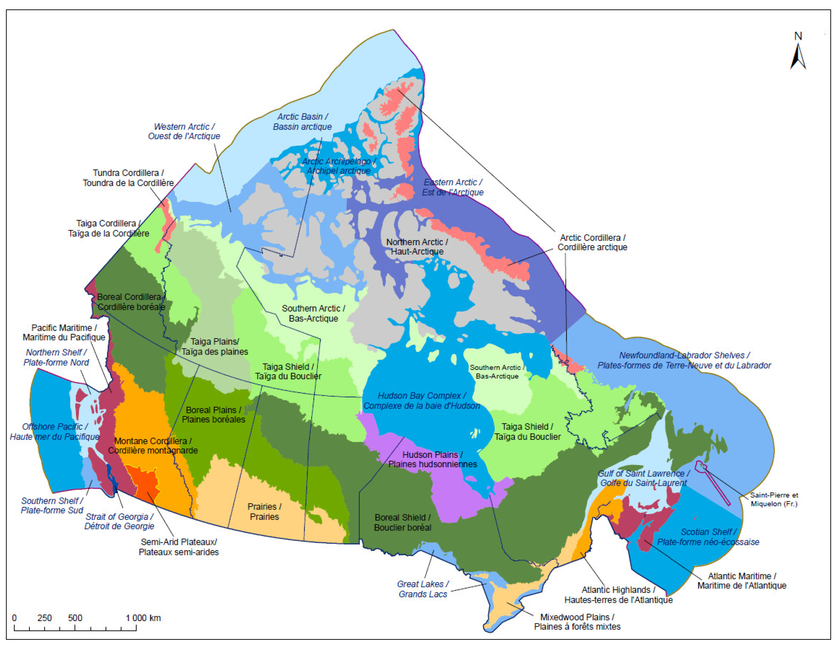
- Li, T.; Helie, R. Eco-regions of Canada. Canadian Council on Ecological Areas (CCEA): Canada, 2014. Available online: https://www.ccea.org/Downloads/shapefiles/CA_ecozones_15M_v5_final_map%20v20140213.pdf (accessed on 12 October 2020).
- Dunne, T.; Leopold, L.B. Water in Environmental Planning; W.H. Freeman: San Francisco, CA, USA, 1978; p. 818. [Google Scholar]
- Frankenberger, J.R.; Brooks, E.S.; Walter, M.T.; Walter, M.F.; Steenhuis, T.S. A GIS-based variable source area model. Hydrol. Process. 1999, 13, 804–822. [Google Scholar] [CrossRef]
- Walter, M.T.; Walter, M.F.; Brooks, E.S.; Steenhuis, T.S.; Boll, J.; Weiler, K.R. Hydrologically sensitive areas: Variable source area hydrology implications for water quality risk assessment. J. Soil Water Conserv. 2000, 3, 277–284. [Google Scholar]
- Merwin, I.A.; Stiles, W.C.; Van Es, H.M. Orchard Groundcover Management Impacts on Soil Physical Properties. J. Am. Soc. Hortic. Sci. 1994, 119, 216–222. [Google Scholar] [CrossRef] [Green Version]
- Horton, R.E. An Approach Toward a Physical Interpretation of Infiltration-Capacity. Soil Sci. Soc. Am. J. 1941, 5, 399–417. [Google Scholar] [CrossRef]
- Hewlett, J.D.; Hibbert, A.R. Moisture and energy conditions within a sloping soil mass during drainage. J. Geophys. Res. 1963, 68, 1081–1087. [Google Scholar] [CrossRef] [Green Version]
- Hornbeck, J.W.; Reinhart, K.G. Water quality and soil erosion as affected by logging in steep terrain. J. Soil Water Conserv. 1964, 19, 23–27. [Google Scholar]
- Whipkey, R.Z. Subsurface stormflow from forested slopes Bull. Int. Assoc. Sci. Hydrol. 1965, 10, 74–85. [Google Scholar] [CrossRef] [Green Version]
- Garen, D.C.; Moore, D.S. Curve Number Hydrology in Water Quality Modeling: Uses, Abuses, and Future Directions. JAWRA J. Am. Water Resour. Assoc. 2005, 41, 377–388. [Google Scholar] [CrossRef]
- Knisel, W.G. CREAMS: A Field Scale Model for Chemicals, Runoff, and Erosion from Agricultural Management Systems; Department of Agriculture, Science and Education Administration: Washington, DC, USA, 1980; Available online: https://agris.fao.org/agris-search/search.do?recordID=US8025878 (accessed on 12 October 2020).
- Soil Conservation Service National Engineering Handbook, section 4, Hydrology. 1969. Available online: https://www.nrcs.usda.gov/wps/portal/nrcs/detail/?cid=nrcs141p2_024573 (accessed on 12 October 2020).
- Steenhuis, T.S.; Winchell, M.; Rossing, J.; Zollweg, J.A.; Walter, M.F. SCS Runoff Equation Revisited for Variable-Source Runoff Areas. J. Irrig. Drain. Eng. 1995, 121, 234–238. [Google Scholar] [CrossRef]
- Hjelmfelt, A.T., Jr. Curve number procedure as infiltration method. J. Hydraul. Div. 1980, 106, 1107–1111. [Google Scholar]
- Mishra, S.K.; Singh, V.P. Long-term hydrological simulation based on the Soil Conservation Service curve number. Hydrol. Process. 2004, 18, 1291–1313. [Google Scholar] [CrossRef]
- Shook, K.R.; Pomeroy, J.W.; Spence, C.; Boychuk, L. Storage dynamics simulations in prairie wetland hydrology models: Evaluation and parameterization. Hydrol. Process. 2013, 27, 1875–1889. [Google Scholar] [CrossRef]
- Kiesel, J.; Fohrer, N.; Schmalz, B.; White, M.J. Incorporating landscape depressions and tile drainages of a northern German lowland catchment into a semi-distributed model. Hydrol. Process. 2010, 24, 1472–1486. [Google Scholar] [CrossRef]
- Almendinger, J.E.; Murphy, M.S.; Ulrich, J.S. Use of the Soil and Water Assessment Tool to Scale Sediment Delivery from Field to Watershed in an Agricultural Landscape with Topographic Depressions. J. Environ. Qual. 2014, 43, 9–17. [Google Scholar] [CrossRef] [PubMed]
- Mekonnen, B.A.; Mazurek, K.A.; Putz, G. Sediment Export Modeling in Cold-Climate Prairie Watersheds. J. Hydrol. Eng. 2016, 21, 05016005. [Google Scholar] [CrossRef]
- Mekonnen, B.A.; Mazurek, K.A.; Putz, G. Incorporating landscape depression heterogeneity into the Soil and Water Assessment Tool (SWAT) using a probability distribution. Hydrol. Process. 2016, 30, 2373–2389. [Google Scholar] [CrossRef]
- Crumpton, W.G.; Goldsborough, L.G. Nitrogen transformation and fate in prairie wetlands. Gt. Plains Res. 1998, 8, 57–72. [Google Scholar]
- Granger, R.J.; Gray, D.M.; Dyck, G.E. Snowmelt infiltration to frozen Prairie soils. Can. J. Earth Sci. 1984, 21, 669–677. [Google Scholar] [CrossRef] [Green Version]
- Gray, D.M.; Toth, B.; Zhao, L.; Pomeroy, J.W.; Granger, R.J. Estimating areal snowmelt infiltration into frozen soils. Hydrol. Process. 2001, 15, 3095–3111. [Google Scholar] [CrossRef]
- Aldrich, J.W.; Slaughter, C.W. Soil erosion on subarctic forest slopes. J. Soil Water Conserv. 1983, 38, 115–118. [Google Scholar]
- Wall, G.J.; Dickinson, W.T.; Rudra, R.P.; Coote, D.R. Seasonal soil erodibility variation in southwestern ontario. Can. J. Soil Sci. 1988, 68, 417–424. [Google Scholar] [CrossRef] [Green Version]
- Kirby, P.C.; Mehuys, G.R. Seasonal variation of soil erodibilities in southwestern Quebec. J. Soil Water Conserv. 1987, 42, 211–215. [Google Scholar]
- Asare, S.N.; Rudra, R.P.; Dickinson, W.T.; Wall, G.J. Seasonal Variability of Hydraulic Conductivity. Trans. ASAE 1993, 36, 451–457. [Google Scholar] [CrossRef]
- Tiessen, K.; Elliott, J.; Yarotski, J.; Lobb, D.A.; Flaten, D.N.; Glozier, N.E. Conventional and Conservation Tillage: Influence on Seasonal Runoff, Sediment, and Nutrient Losses in the Canadian Prairies. J. Environ. Qual. 2010, 39, 964–980. [Google Scholar] [CrossRef] [Green Version]
- Ferrick, M.G.; Gatto, L.W. Quantifying the effect of a freeze-thaw cycle on soil erosion: Laboratory experiments. Earth Surf. Process. Landf. 2005, 30, 1305–1326. [Google Scholar] [CrossRef]
- Dagesse, D.F. Freezing cycle effects on water stability of soil aggregates. Can. J. Soil Sci. 2013, 93, 473–483. [Google Scholar] [CrossRef]
- Donnan, W.W. An overview of drainage worldwide. In Proceedings of the 3rd National Drainage Symposium, Chicago, IL, USA, 6–9 December 1976. [Google Scholar]
- USDA. Water—Yearbook of Agriculture; United States Department of Agriculture: Washington, DC, USA, 1955.
- Lrwin, R.W.; Clayton, R.C. Drainage Guide for Ontario; Ministry of Agriculture, Food and Rural Affairs (OMAFRA): Toronto, ON, Canada, 1978.
- OMAFRA 1996. Census of Agriculture and Policy & Programs Branch; Ontario Ministry of Agriculture, Food, and Rural Affairs: Toronto, ON, Canada, 1996.
- Zhang, T.Q.; Hu, Q.C.; Wang, Y.T.; Tan, C.S.; O’Halloran, I.; Drury, C.F.; Reid, D.K.; Ball-Coelho, B.; Ma, B.L.; Welacky, T.; et al. Determination of Some Key Factors for Ontario Soil P Index and Effectiveness of Manure Application Practices for Mitigating Risk to Water Resources; Report NM8002 to the Nutrient Management Joint Research Program; Ontario Ministry of Agriculture, Food and Rural Affairs, Ontario Ministry of Environment: Guelph, ON, Canada, 2009. [Google Scholar]
- Culley, J.L.B.; Bolton, E.F.; Bernyk, V. Suspended Solids and Phosphorus Loads from a Clay Soil: I. Plot Studies. J. Environ. Qual. 1983, 12, 493–498. [Google Scholar] [CrossRef]
- Gaynor, J.D.; Findlay, W.I. Soil and Phosphorus Loss from Conservation and Conventional Tillage in Corn Production. J. Environ. Qual. 1995, 24, 734–741. [Google Scholar] [CrossRef]
- Simard, R.R.; Beauchemin, S.; Haygarth, P.M. Potential for Preferential Pathways of Phosphorus Transport. J. Environ. Qual. 2000, 29, 97–105. [Google Scholar] [CrossRef]
- Kinley, R.D.; Gordon, R.J.; Stratton, G.W.; Patterson, G.T.; Hoyle, J. Phosphorus Losses through Agricultural Tile Drainage in Nova Scotia, Canada. J. Environ. Qual. 2007, 36, 469–477. [Google Scholar] [CrossRef] [Green Version]
- Eastman, M.; Gollamudi, A.; Stämpfli, N.; Madramootoo, C.; Sarangi, A. Comparative evaluation of phosphorus losses from subsurface and naturally drained agricultural fields in the Pike River watershed of Quebec, Canada. Agric. Water Manag. 2010, 97, 596–604. [Google Scholar] [CrossRef]
- Tan, C.; Zhang, T.Q. Surface runoff and sub-surface drainage phosphorus losses under regular free drainage and controlled drainage with sub-irrigation systems in southern Ontario. Can. J. Soil Sci. 2011, 91, 349–359. [Google Scholar] [CrossRef]
- Reid, D.K.; Ball, B.; Zhang, T.Q. Accounting for the Risks of Phosphorus Losses through Tile Drains in a Phosphorus Index. J. Environ. Qual. 2012, 41, 1720–1729. [Google Scholar] [CrossRef] [PubMed]
- Hooghoudt, S.B. Contributions to the knowledge of some physical constants of the soil. Versl. Landbouwkd. Onderz. 1940, 46, 515–707. (In Dutch) [Google Scholar]
- Kirkham, D. Theory of land drainage In: Drainage of agricultural lands. Agron. Monogr. 1957. Available online: https://acsess.onlinelibrary.wiley.com/doi/book/10.2134/agronmonogr7 (accessed on 12 October 2020).
- Golmohammadi, G.; Prasher, S.O.; Madani, A.; Rudra, R.P.; Youssef, M.A. SWATDRAIN, a new model to simulate the hydrology of agricultural Lands, model development and evaluation. Biosyst. Eng. 2016, 141, 31–47. [Google Scholar] [CrossRef]
- Koch, S.; Bauwe, A.; Lennartz, B. Application of the SWAT Model for a Tile-Drained Lowland Catchment in North-Eastern Germany on Subbasin Scale. Water Resour. Manag. 2012, 27, 791–805. [Google Scholar] [CrossRef]
- Bauwe, A.; Eckhardt, K.-U.; Lennartz, B. Predicting dissolved reactive phosphorus in tile-drained catchments using a modified SWAT model. Ecohydrol. Hydrobiol. 2019, 19, 198–209. [Google Scholar] [CrossRef]
- Coelho, B.B.; Lapen, D.; Murray, R.; Topp, E.; Bruin, A.; Khan, B. Nitrogen loading to offsite waters from liquid swine manure application under different drainage and tillage practices. Agric. Water Manag. 2012, 104, 40–50. [Google Scholar] [CrossRef]
- Coelho, B.B.; Murray, R.; Lapen, D.; Topp, E.; Bruin, A. Phosphorus and sediment loading to surface waters from liquid swine manure application under different drainage and tillage practices. Agric. Water Manag. 2012, 104, 51–61. [Google Scholar] [CrossRef]
- Her, Y.G.; Chaubey, I.; Frankenberger, J.; Jeong, J. Implications of spatial and temporal variations in effects of conservation practices on water management strategies. Agric. Water Manag. 2017, 180, 252–266. [Google Scholar] [CrossRef]
- Gupta, A.K.; Rudra, R.P.; Gharabaghi, B.; Daggupati, P.; Goel, P.K.; Shukla, R. CoBAGNPS: A toolbox for simulating water and sediment control basin, WASCoB through AGNPS model. CATENA 2019, 179, 49–65. [Google Scholar] [CrossRef]
- Fiener, P.; Auerswald, K.; Weigand, S. Managing erosion and water quality in agricultural watersheds by small detention ponds. Agric. Ecosyst. Environ. 2005, 110, 132–142. [Google Scholar] [CrossRef]
- Shrestha, N.K.; Leta, O.T.; De Fraine, B.; Van Griensven, A.; Bauwens, W. OpenMI-based integrated sediment transport modelling of the river Zenne, Belgium. Environ. Model. Softw. 2013, 47, 193–206. [Google Scholar] [CrossRef]
- Yang, W.L.; Simmons, J.; Oginskyy, A.; McKague, K. SWAT Modelling of Agricultural BMPs and Analysis of BMP Cost Effectiveness in the Gully Creek Watershed; OMAFRA: Norfolk, ON, Canada, 2013.
- Heathwaite, L.; Reaney, S.; Lane, S. Understanding spatial signals in catchments: Linking critical areas, identifying connection and evaluating response. In Proceedings of the 5th International Phosphorus Workshop, Silkeborg, Denmark, 3–7 September 2007; p. 25. [Google Scholar]
- Yen, H.; Daggupati, P.; White, M.J.; Srinivasan, R.; Gossel, A.; Wells, D.; Arnold, J.G. Application of Large-Scale, Multi-Resolution Watershed Modeling Framework Using the Hydrologic and Water Quality System (HAWQS). Water 2016, 8, 164. [Google Scholar] [CrossRef]
- Zhang, B.; Shrestha, N.K.; Rudra, R.; Shukla, R.; Daggupati, P.; Goel, P.; Dickinson, W.; Allataifeh, N. Threshold storm approach for locating phosphorus problem areas: An application in three agricultural watersheds in the Canadian Lake Erie basin. J. Great Lakes Res. 2020, 46, 132–143. [Google Scholar] [CrossRef]
- Alilou, H.; Moghaddamnia, A.; Keshtkar, H.; Han, D.; Bray, M. A cost-effective and efficient framework to determine water quality monitoring network locations. Sci. Total. Environ. 2018, 624, 283–293. [Google Scholar] [CrossRef] [Green Version]
- Shrestha, N.K.; Punzal, C.; Leta, O.T.; Bauwens, W. Trace Metal Modelling of a Complex River Basin Using the Suite of Models Integrated in the OpenMI Platform. Environments 2018, 5, 48. [Google Scholar] [CrossRef] [Green Version]
- Van Griensven, A.; Vandenberghe, V.; Bols, J.; De Pauw, N.; Goethals, P.; Meirlaen, J.; Vanrolleghem, P.A.; Van Vooren, L.; Bauwens, W. Experience and organistation of automated measuring stations for river water quality monitoring. 2000. Available online: https://www.semanticscholar.org/paper/Experience-and-organisation-of-automated-measuring-Griensven-Vandenberghe/9ca1d609e857aae8cdee97fe729abe8abfc4f50f (accessed on 12 October 2020).
- Anderson, C.W.; Rounds, S.A. Use of Continuous Monitors and Autosamplers to Predict Unmeasured Waterquality Constituents in Tributaries of the Tualatin River, Oregon; U.S. Geological Survey Scientific Investigations Report; US Department of the Interior, US Geological Survey: Reston, VA, USA, 2010; Volume 5008, p. 76.


| References | Model Used and Location of Study Area | Scale of Application and Modeling Approach |
|---|---|---|
| Arabi et al., [110] | SWAT, Northeast Indiana, USA, Black Creek Basin | Field scale, but connectivity of HRUs not considered |
| Bello et al., [111] | BASINS/HSPF, Malaysia, Skudai watershed | Watershed (287 km2), CSAs identified in present and future land use scenarios |
| Cho et al., [112] | SWAT, Georgia, USA; Little River Experimental Watershed | Watershed scale (334 km2); both stream order based and HRU based scenarios are done. CSAs identified at HRU level |
| Ghebremichael et al., [113] | SWAT, Vermont, USA; Rock River Watershed of Lake Champlain | CSAs are identified at HRU level, connectivity not considered |
| Ghebremichael et al., [114] | SWAT, USA; Rock River Watershed & Cannonsville Reservoir Watershed | Field scale (0.027–0.04 km2), connection between HRUs not considered |
| Guo et al., [115] | SWAT, China; Miyun Reservoir Watershed | Watershed scale (4888 km2), connection between HRUs not considered |
| Ning et al., [116] | GWLF, Kao-Ping River Basin, South Taiwan | Watershed scale (3256 km2) |
| Niraula et al., [117] | SWAT, USA; Saugahatchee Creek Watershed & Magnolia River Watershed | CSAs identified at HRU level |
| Niraula et al., [45] | SWAT and GWLF, Alabama, USA; Saugahatchee Creek Watershed | Study area of 570 km2, CSAs identified at sub-basin level |
| Ouyoung et al., [118] | SWAT, China; Bahe River Watershed | CSAs identified at sub-basin level |
| Panagopoulos et al., [119] | SWAT, Greece; Arachthos Catchment | CSAs identified at HRU level |
| Pease et al., [120] | AnnAGNPS, North Dakota, USA, Pipestem Creek | Watershed scale (1697 km2) |
| Rousseau et al., [121] | GIBSI, Quebec, Canada, Beaurivage River Basin | Watershed scale (718 km2) |
| Shang et al., [122] | SWAT, China; Lake Erhai Basin | CSAs are identified at sub-basin level |
| Shrestha et al., [123] | AGNPS, Canada, Holtby watershed | Watershed (3.74 km2), CSAs identified at cell level |
| Tripathi et al., [124] | SWAT, Bihar, India; Nagwan Watershed | Watershed (92.46 km2), CSAs are identified at sub-watershed level |
| Wang and Lin, [125] | AnnAGNPS, China, Dage subwatershed of Chaohe River | Watershed (1876 km2) |
| Winchell et al., [50] | SWAT, USA-CAN border; Lake Champlain Missisquoi Bay Watershed | Watershed (310 km2), CSAs identified at HRU level, considers saturation excess using topographic index |
| White et al., [126] | SWAT, Oklahoma, USA; 6 different watersheds | Watershed (23,000–174,000 km2), CSAs are identified at HRU level |
© 2020 by the authors. Licensee MDPI, Basel, Switzerland. This article is an open access article distributed under the terms and conditions of the Creative Commons Attribution (CC BY) license (http://creativecommons.org/licenses/by/4.0/).
Share and Cite
Rudra, R.P.; Mekonnen, B.A.; Shukla, R.; Shrestha, N.K.; Goel, P.K.; Daggupati, P.; Biswas, A. Currents Status, Challenges, and Future Directions in Identifying Critical Source Areas for Non-Point Source Pollution in Canadian Conditions. Agriculture 2020, 10, 468. https://doi.org/10.3390/agriculture10100468
Rudra RP, Mekonnen BA, Shukla R, Shrestha NK, Goel PK, Daggupati P, Biswas A. Currents Status, Challenges, and Future Directions in Identifying Critical Source Areas for Non-Point Source Pollution in Canadian Conditions. Agriculture. 2020; 10(10):468. https://doi.org/10.3390/agriculture10100468
Chicago/Turabian StyleRudra, Ramesh P., Balew A. Mekonnen, Rituraj Shukla, Narayan Kumar Shrestha, Pradeep K. Goel, Prasad Daggupati, and Asim Biswas. 2020. "Currents Status, Challenges, and Future Directions in Identifying Critical Source Areas for Non-Point Source Pollution in Canadian Conditions" Agriculture 10, no. 10: 468. https://doi.org/10.3390/agriculture10100468