
Production Systems with Parallel Heterogeneous Servers of Limited Capacity: Accurate Modeling and Performance Analysis


Abstract
:1. Introduction
2. Methodology of Parallel System Modeling
2.1. Loss in Parallel Systems without Queue
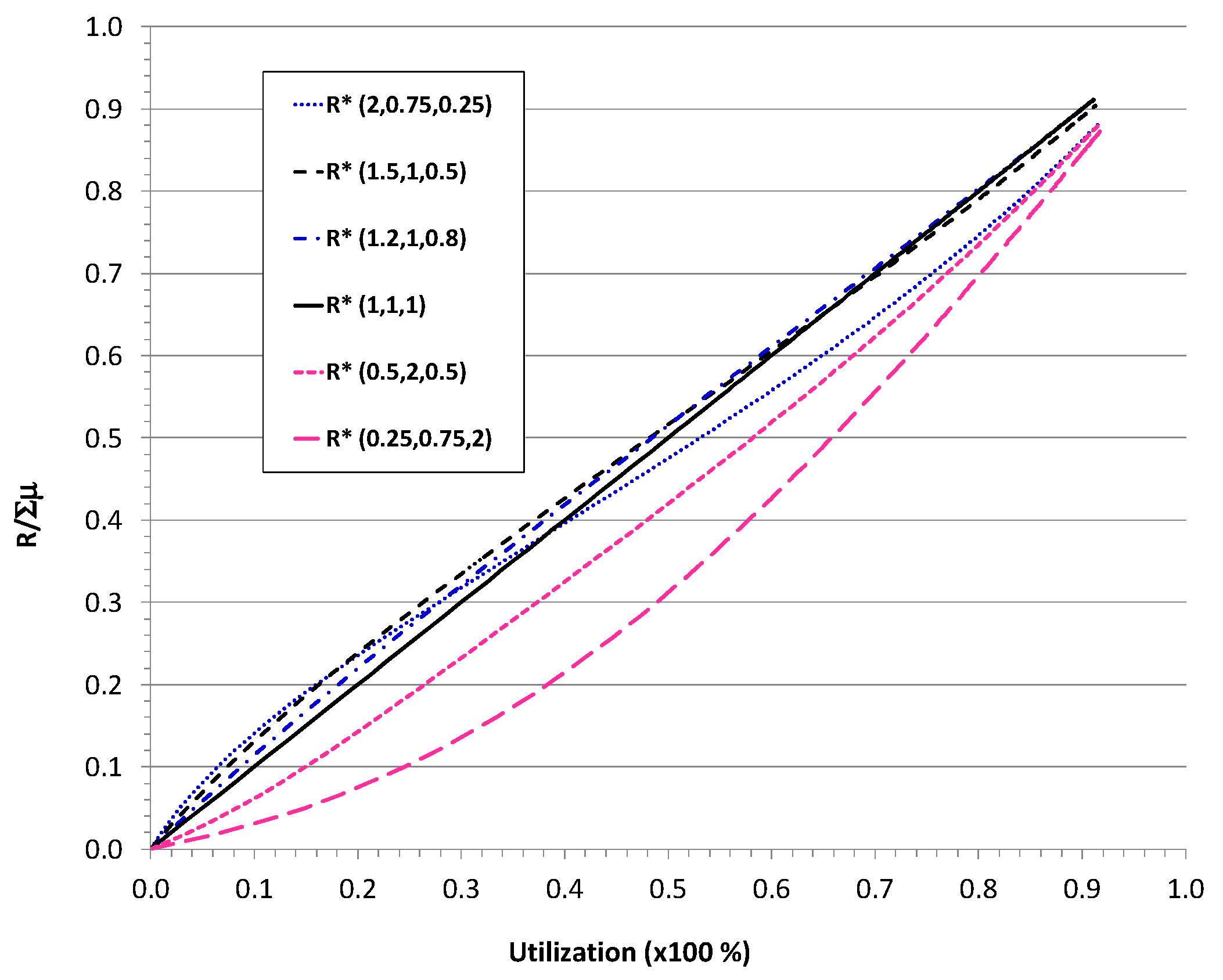
2.2. System of Heterogeneous Parallel Servers
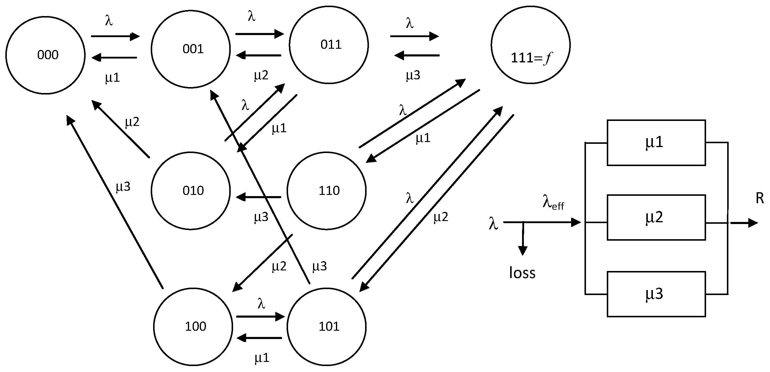
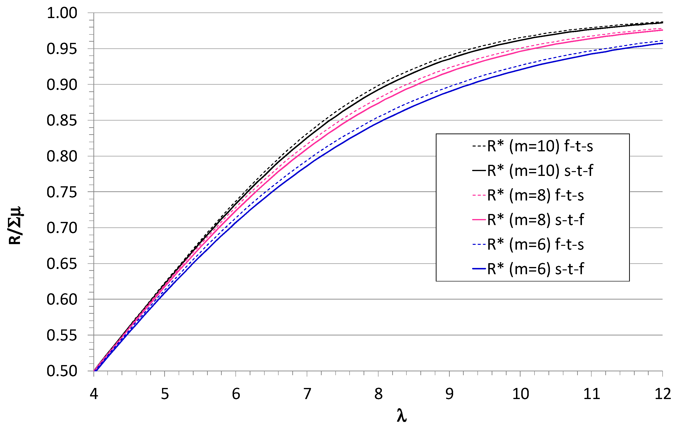
3. Parallel Heterogeneous Servers with a Common Waiting Queue
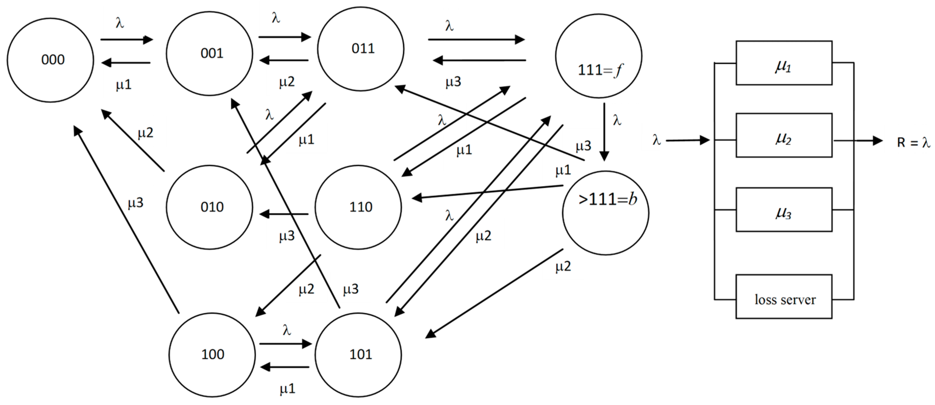
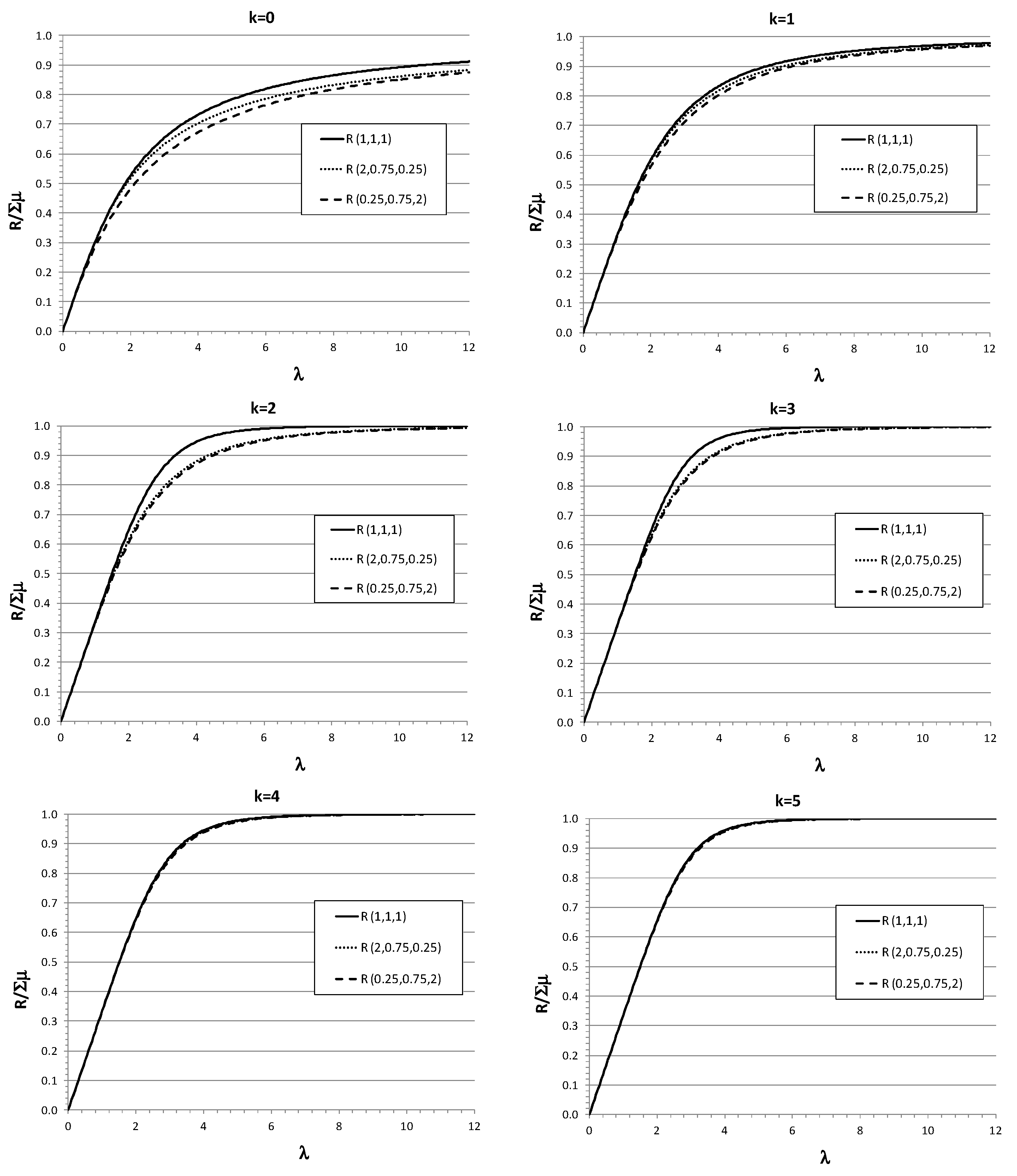
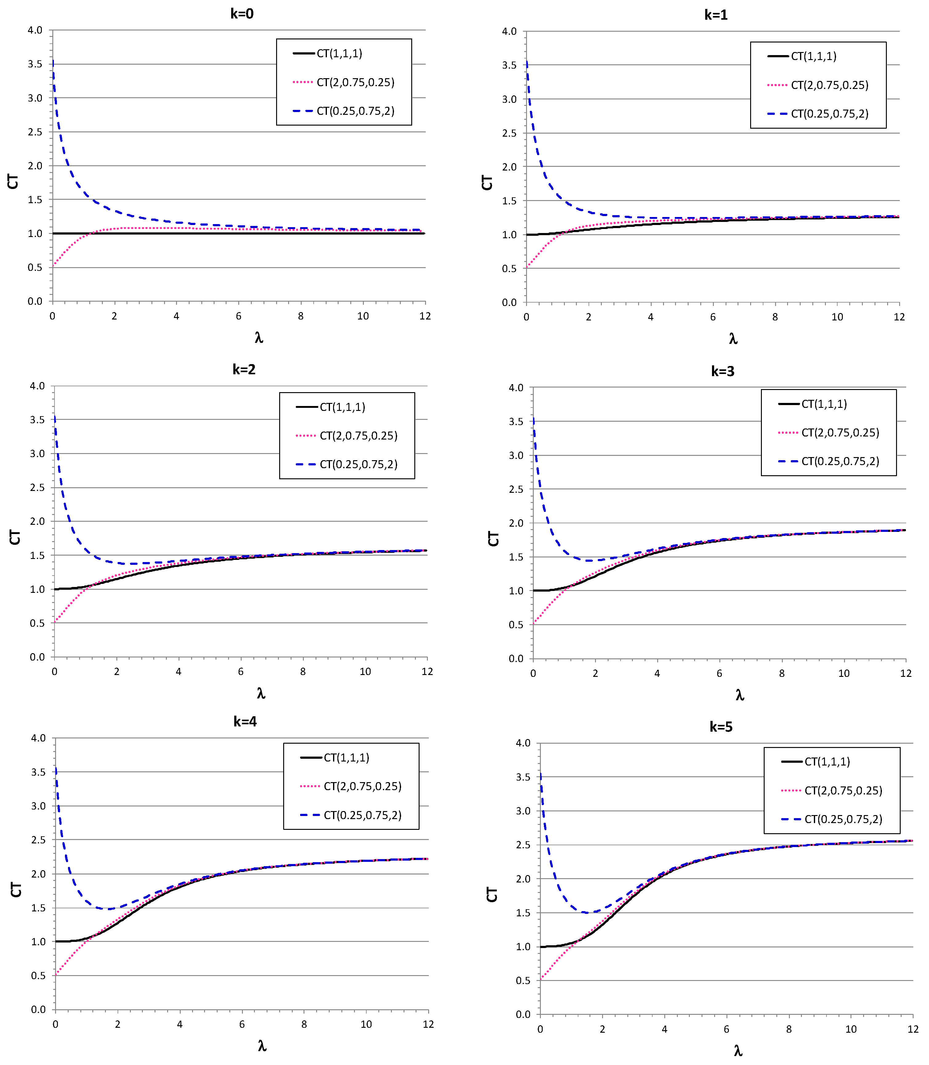
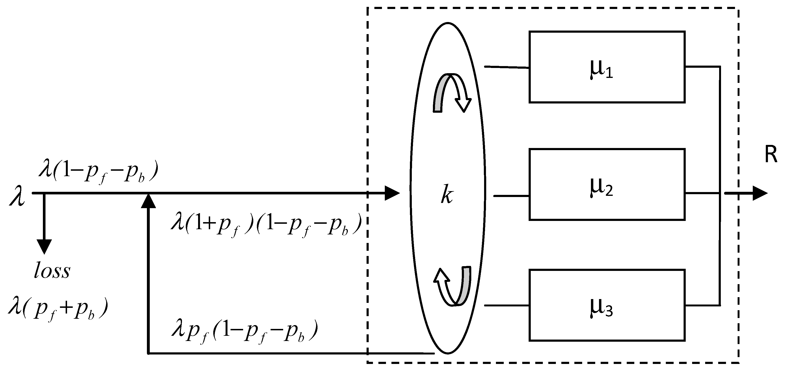
4. Systems of Parallel Heterogeneous Servers with Recirculation
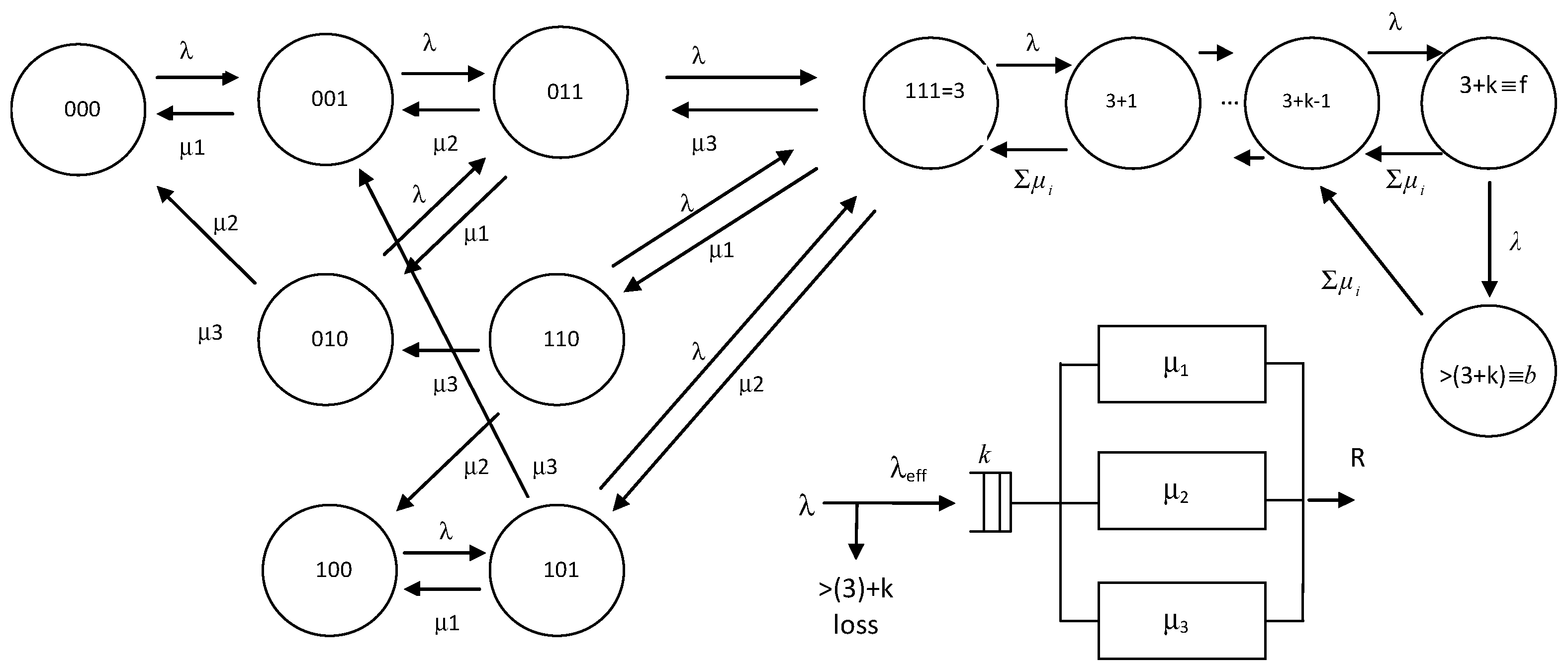
5. Hybrid Modeling of Heterogeneous Servers with General Service Time Distributions
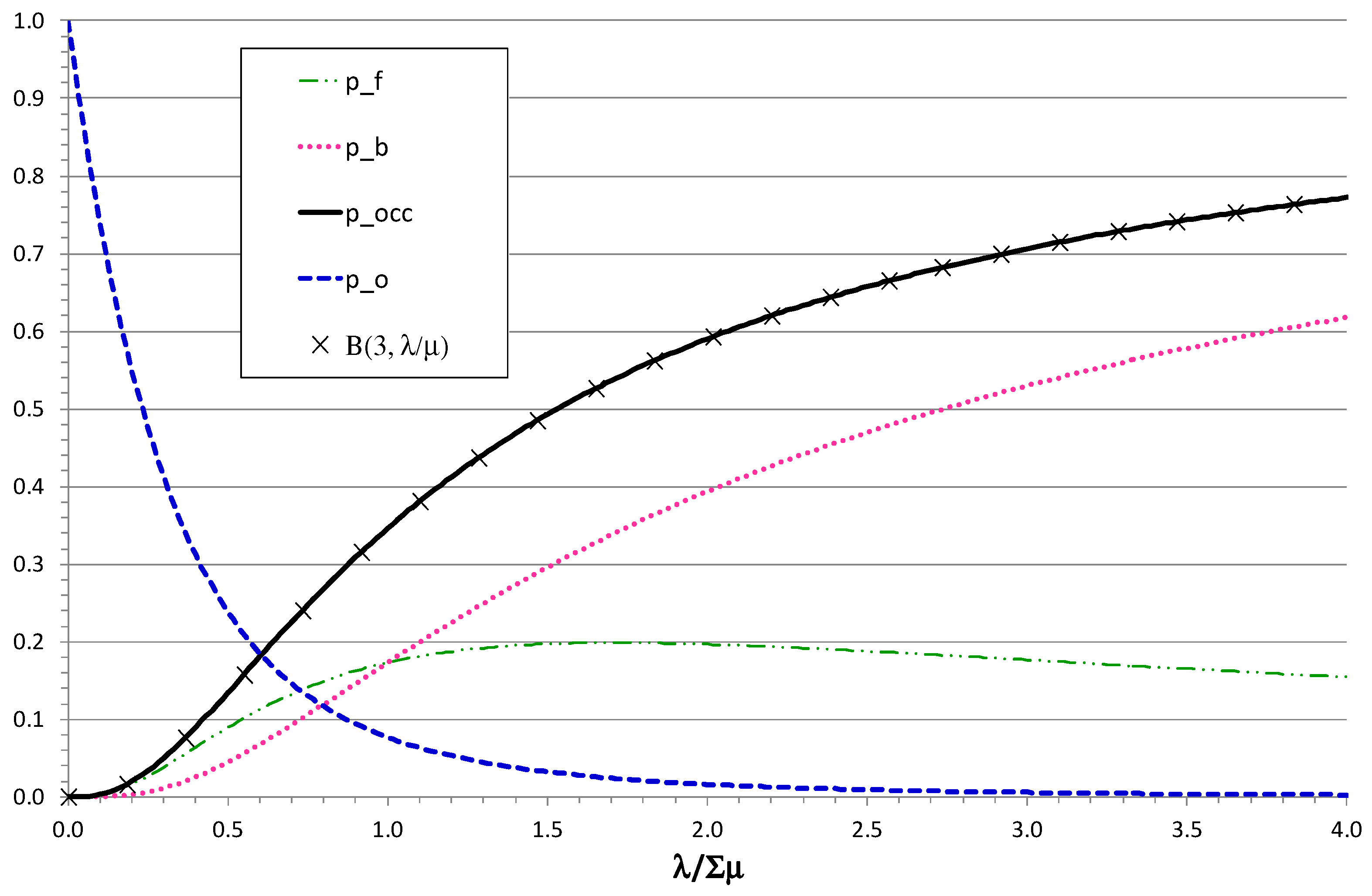
5.1. Uncertainty of the Offered Load
5.2. Application to Non-Exponential Service Time Distributions
6. Conclusions
Author Contributions
Funding
Data Availability Statement
Conflicts of Interest
References
- Curry, G.L.; Feldman, R.M. Manufacturing Systems Modelling and Analysis; Springer Science & Business Media: Berlin/Heidelberg, Germany, 2010. [Google Scholar]
- Smith, J.M. Introduction to Queuing Networks: Theory ∩ Practice; Springer: Berlin/Heidelberg, Germany, 2018. [Google Scholar]
- Shortle, J.F.; Thompson, J.M.; Gross DHarris, C.M. Fundamentals of Queueing Theory; John Wiley & Sons: Hoboken, NJ, USA, 2018. [Google Scholar]
- Efrosinin, D. Controlled Queueing Systems with Heterogeneous Servers. 2004. Available online: https://d-nb.info/971824401/34 (accessed on 1 December 2023).
- Wolff, R.W. Poisson arrivals see time averages. Oper. Res. 1982, 30, 223–231. [Google Scholar] [CrossRef]
- Gans, N.; Koole, D.; Mandelbaum, A. Telephone call centers: Tutorial, review, and research prospects. Manuf. Serv. Oper. Manag. 2003, 5, 79–141. [Google Scholar] [CrossRef]
- Armony, M.; Ward, A.R. Fair dynamic routing in large-scale heterogeneous-server systems. Oper. Res. 2010, 58, 624–637. [Google Scholar] [CrossRef]
- Gumbel, H. Waiting lines with heterogeneous servers. Oper. Res. 1960, 8, 504–511. [Google Scholar] [CrossRef]
- Disney, R.L. Some multichannel queueing problems with ordered entry. J. Ind. Eng. 1962, 13, 46–48. [Google Scholar]
- Disney, R.L. Some Multichannel Queueing Problems with Ordered Entry—An Application to Conveyor Theory. J. Ind. Eng. 1963, 14, 105–108. [Google Scholar]
- Singh, W.S. Two-server Markovian queues with balking: Heterogeneous vs. homogeneous servers. Oper. Res. 1970, 18, 145–159. [Google Scholar] [CrossRef]
- Singh, V.S. Markovian queues with three heterogeneous servers. IIE Trans. 1971, 3, 45–48. [Google Scholar] [CrossRef]
- Elsayed, E.A. Multichannel queueing systems with ordered entry and finite source. Comput. Oper. Res. 1983, 10, 213–222. [Google Scholar] [CrossRef]
- Yao, D.D. The arrangement of servers in an ordered-entry system. Oper. Res. 1987, 35, 759–763. [Google Scholar] [CrossRef]
- Yao, D.A. Convexity properties of the overflow in an ordered-entry system with heterogeneous servers. Oper. Res. Lett. 1986, 5, 145–147. [Google Scholar] [CrossRef]
- Saglam, V.; Shahbazov, A. Minimizing loss probability in queuing systems with heterogeneous servers. Iran. J. Sci. Technol. Trans. A Sci. 2007, 31, 199–206. [Google Scholar]
- Boxma, O.J.; Koole, G.M.; Liu, Z. Queueing-Theoretic Solution Methods for Models of Parallel and Distributed Systems. Centrum voor Wiskunde in Informatica, Department of Operations Research, Statistics, and System Theory. 1994. Available online: https://ir.cwi.nl/pub/5133 (accessed on 1 December 2023).
- Isguder, H.O.; Uzunoglu-Kocer, U. Analysis of GI/M/n/n queueing system with ordered entry and no waiting line. Appl. Math. Model. 2014, 38, 1024–1032. [Google Scholar] [CrossRef]
- Melikov, A.Z.; Ponomarenko, L.A.; Mekhbaliyeva, E.V. Analyzing the models of systems with heterogeneous servers. Cybern. Syst. Anal. 2020, 56, 89–99. [Google Scholar] [CrossRef]
- Cooper, R.B. Queues with ordered servers that work at different rates. Oper. Res. 1976, 13, 69–78. [Google Scholar] [CrossRef]
- Matsui, M.; Fukuta, J. On a Multichannel Queueing System with Ordered Entry and Heterogeneous Servers. AIIE Trans. 1977, 9, 209–214. [Google Scholar] [CrossRef]
- Nath, G.B.; Enns, E.G. Optimal service rates in the multiserver loss system with heterogeneous servers. J. Appl. Probab. 1981, 18, 776–781. [Google Scholar] [CrossRef]
- Pourbabai, B.; Sonderman, D. Service utilization factors in queueing loss systems with ordered entry and heterogeneous servers. J. Appl. Probab. 1986, 23, 236–242. [Google Scholar] [CrossRef]
- Muth, E.J.; White, J.A. Conveyor theory: A survey. AIIE Trans. 1979, 11, 270–277. [Google Scholar] [CrossRef]
- Nazzal, D.; El-Nashar, A. Winter Simulation Conference—Survey of research in modeling conveyor-based automated material handling systems in wafer fabs. In Proceedings of the 2007 Winter Simulation Conference, Washington, DC, USA, 9–12 December 2007; pp. 1781–1788. [Google Scholar] [CrossRef]
- Nawijn, W.M. A note on many-server queueing systems with ordered entry, with an application to conveyor theory. J. Appl. Probab. 1983, 20, 144–152. [Google Scholar] [CrossRef]
- Nawijn, W.M. On a two-server finite queuing system with ordered entry and deterministic arrivals. Eur. J. Oper. Res. 1984, 18, 388–395. [Google Scholar] [CrossRef]
- Pourbabai, B. Markovian queueing systems with retrials and heterogeneous servers. Comput. Math. Appl. 1987, 13, 917–923. [Google Scholar] [CrossRef]
- Boysen, N.; Briskorn, D.; Fedtke, S.; Schmickerath, M. Automated sortation conveyors: A survey from an operational research perspective. Eur. J. Oper. Res. 2019, 276, 796–815. [Google Scholar] [CrossRef]
- Sonderman, D. An analytical model for recirculating conveyors with stochastic inputs and outputs. Int. J. Prod. Res. 1982, 20, 591–605. [Google Scholar] [CrossRef]
- Schmidt, L.C.; Jackman, J. Modeling recirculating conveyors with blocking. Eur. J. Oper. Res. 2000, 124, 422–436. [Google Scholar] [CrossRef]
- Brandwajn, A.; Jow, Y. An approximation method for tandem queues with blocking. Oper. Res. 1988, 36, 73–83. [Google Scholar] [CrossRef]
- Hsieh, Y.J.; Bozer, Y.A. Analytical modeling of closed-loop conveyors with load recirculation. In International Conference on Computational Science and Its Applications; Springer: Berlin/Heidelberg, Germany, 2005. [Google Scholar] [CrossRef]
- Haghighi, A.M.; Mishev, D.P. A parallel priority queueing system with finite buffers. J. Parallel Distrib. Comput. 2006, 66, 379–392. [Google Scholar] [CrossRef]
- Van der Gaast, J.P.; De Koster, M.B.M.; Adan, I.J. Conveyor merges in zone picking systems: A tractable and accurate approximate model. Transp. Sci. 2018, 52, 1428–1443. [Google Scholar] [CrossRef]
- Burke, P.J. The output of a queuing system. Oper. Res. 1956, 4, 699–704. [Google Scholar] [CrossRef]
- Armony, M. Dynamic routing in large-scale service systems with heterogeneous servers. Queueing Syst. 2005, 51, 287–329. [Google Scholar] [CrossRef]
- Pike, R.; Martin, G.E. The bowl phenomenon in unpaced lines. Int. J. Prod. Res. 1994, 32, 483–499. [Google Scholar] [CrossRef]
- Bolotin, V. Telephone circuit holding time distributions. In 14th International Teletraffic Congress; The Fundamental Role of Teletraffic in the Evolution of Telecommunications Networks, Labetoulle, J., Roberts, J.W., Eds.; Elsevier: Amsterdam, The Netherlands, 2014. [Google Scholar]


| Arrival Rate | Service Rates | Simul | Erlang-B | Model A | Model B | Simul vs. Model A | Simul vs. Model B | |
|---|---|---|---|---|---|---|---|---|
| λ | (μ1, μ2, μ3) | Mean | Half Width | (%) | (%) | |||
| 0.1 | (1, 1, 1) | 0.0332 | 0.0002 | 0.0333 | 0.0333 | 0.0333 | −0.40 | −0.39 |
| 0.5 | 0.1644 | 0.0003 | 0.1646 | 0.1665 | 0.1646 | −1.25 | −0.08 | |
| 1 | 0.3125 | 0.0004 | 0.3125 | 0.3254 | 0.3125 | −4.14 | −0.01 | |
| 3 | 0.6540 | 0.0009 | 0.6538 | 0.6838 | 0.6538 | −4.55 | 0.03 | |
| 5 | 0.7838 | 0.0014 | 0.7839 | 0.8035 | 0.7839 | −2.51 | −0.01 | |
| 10 | 0.8936 | 0.0014 | 0.8931 | 0.9004 | 0.8931 | −0.76 | 0.05 | |
| 30 | 0.9656 | 0.0032 | 0.9657 | 0.9567 | 0.9657 | 0.93 | 0.00 | |
| 0.1 | (0.25, 0.75, 2) | 0.0332 | 0.0002 | 0.0333 | 0.0333 | −0.40 | −0.35 | |
| 0.5 | 0.1606 | 0.0002 | 0.1621 | 0.1607 | −0.91 | −0.04 | ||
| 1 | 0.2944 | 0.0005 | 0.2973 | 0.2944 | −0.99 | 0.00 | ||
| 3 | 0.5966 | 0.0008 | 0.5757 | 0.5964 | 3.50 | 0.03 | ||
| 5 | 0.7263 | 0.0013 | 0.6789 | 0.7261 | 6.52 | 0.02 | ||
| 10 | 0.8518 | 0.0016 | 0.7711 | 0.8518 | 9.47 | −0.01 | ||
| 30 | 0.9487 | 0.0031 | 0.8392 | 0.9489 | 11.55 | −0.02 | ||
| 0.1 | (2, 0.75, 0.25) | 0.0332 | 0.0333 | 0.0333 | −0.50 | −0.50 | ||
| 0.5 | 0.1652 | 0.1638 | 0.1652 | 0.84 | −0.03 | |||
| 1 | 0.3138 | 0.2970 | 0.3138 | 5.34 | −0.02 | |||
| 3 | 0.6319 | 0.5396 | 0.6318 | −0.57 | 0.02 | |||
| 5 | 0.7508 | 0.6356 | 0.7513 | 2.12 | −0.07 | |||
| 10 | 0.8630 | 0.7349 | 0.8626 | 14.84 | 0.05 | |||
| 30 | 0.9507 | 0.8223 | 0.9507 | 13.51 | 0.00 | |||
| 0.1 | (1.3, 0.4, 1.3) | 0.0332 | 0.0333 | 0.0333 | −0.30 | −0.30 | ||
| 0.5 | 0.1642 | 0.1637 | 0.1642 | 0.31 | 0.01 | |||
| 1 | 0.3090 | 0.3028 | 0.3090 | 1.99 | −0.01 | |||
| 3 | 0.6367 | 0.5845 | 0.6368 | 8.20 | −0.01 | |||
| 5 | 0.7655 | 0.6922 | 0.7658 | 9.58 | −0.03 | |||
| 10 | 0.8803 | 0.7965 | 0.8798 | 9.52 | 0.05 | |||
| 30 | 0.9604 | 0.8830 | 0.9602 | 8.06 | 0.03 | |||
| 0.1 | (0.5, 2, 0.5) | 0.0332 | 0.0333 | 0.0333 | −0.30 | −0.30 | ||
| 0.5 | 0.1638 | 0.1636 | 0.1639 | 0.10 | −0.04 | |||
| 1 | 0.3070 | 0.3000 | 0.3071 | 2.28 | −0.03 | |||
| 3 | 0.6212 | 0.5279 | 0.6212 | 15.02 | 0.00 | |||
| 5 | 0.7449 | 0.5862 | 0.7451 | 21.31 | −0.02 | |||
| 10 | 0.8614 | 0.6279 | 0.8611 | 27.10 | 0.04 | |||
| 30 | 0.9506 | 0.6541 | 0.9512 | 31.20 | −0.06 | |||
| Dataset Source | λ | (μ1, μ2, μ3) | Loss from Simulation | poverflow M/Mi/k (k = 3) | pocc = pf + pb M/Mi/k/k Model B (k = 3) |
|---|---|---|---|---|---|
| [21] | (1.2, 1, 0.8) | 0.0109 | 0.01086 | ||
| (1, 1.2, 0.8) | 0.0118 | 0.01179 | |||
| 0.5 | (1.2, 0.8, 1) | 0.0119 | 0.01189 | ||
| (0.8, 1.2, 1) | 0.0140 | 0.01402 | |||
| (1, 0.8, 1.2) | 0.0140 | 0.01397 | |||
| (0.8, 1, 1.2) | 0.0152 | 0.01520 | |||
| (1.2, 1, 0.8) | 0.0575 | 0.05749 | |||
| (1, 1.2, 0.8) | 0.0600 | 0.06005 | |||
| 1.0 | (1.2, 0.8, 1) | 0.0609 | 0.06092 | ||
| (0.8, 1.2, 1) | 0.0661 | 0.06611 | |||
| (1, 0.8, 1.2) | 0.0669 | 0.06688 | |||
| (0.8, 1, 1.2) | 0.0696 | 0.06956 | |||
| (1.2, 1, 0.8) | 0.2049 | 0.20490 | |||
| (1, 1.2, 0.8) | 0.2082 | 0.20816 | |||
| 2.0 | (1.2, 0.8, 1) | 0.2094 | 0.20940 | ||
| (0.8, 1.2, 1) | 0.2153 | 0.21533 | |||
| (1, 0.8, 1.2) | 0.2170 | 0.21700 | |||
| (0.8, 1, 1.2) | 0.2198 | 0.21978 | |||
| [18] | 90 | (60, 45, 10) | 0.27166 | 0.2999 | 0.27189 |
| (60, 10, 45) | 0.28577 | 0.1986 | 0.28593 |
| Arrival Rate | Service Rates | Simul | Mod E | Model E vs. Simul | |
|---|---|---|---|---|---|
| λ | (μ1, μ2, μ3) | Mean | Half Width | R* | [%] |
| 1 | (1, 1, 1) | 0.3323 | 0.0005 | 0.3326 | −0.09 |
| 3 | 0.8304 | 0.0009 | 0.8302 | 0.03 | |
| 5 | 0.9629 | 0.0014 | 0.9628 | 0.01 | |
| 1 | (0.25, 0.75, 2) | 0.3320 | 0.0005 | 0.3320 | 0.00 |
| 3 | 0.8174 | 0.0009 | 0.8174 | 0.00 | |
| 5 | 0.9557 | 0.0010 | 0.9553 | 0.05 | |
| 1 | (2, 0.75, 0.25) | 0.3331 | 0.0005 | 0.3326 | 0.13 |
| 3 | 0.8251 | 0.0009 | 0.8250 | 0.00 | |
| 5 | 0.9580 | 0.0013 | 0.9584 | −0.05 | |
| 1 | (1.3, 0.4, 1.3) | 0.3322 | 0.0005 | 0.3325 | −0.09 |
| 3 | 0.8261 | 0.0007 | 0.8262 | −0.01 | |
| 5 | 0.9601 | 0.0011 | 0.9603 | −0.02 | |
| 1 | (0.5, 2, 0.5) | 0.3324 | 0.0005 | 0.3324 | 0.01 |
| 3 | 0.8227 | 0.0009 | 0.8227 | 0.00 | |
| 5 | 0.9576 | 0.0012 | 0.9576 | 0.00 | |
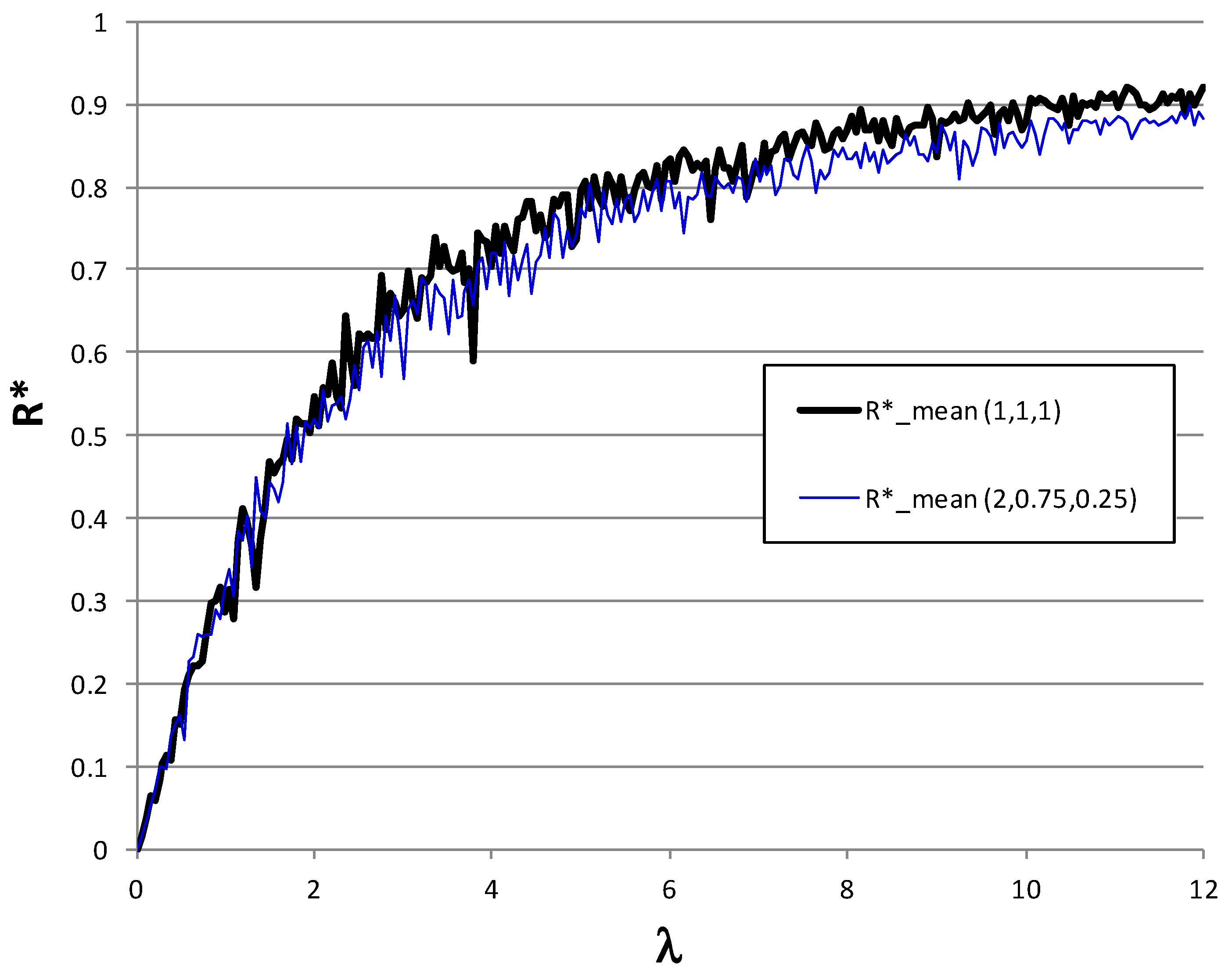
| μ | R* Simul w/o Recirc. | R* Model E | Simul w/o vs. Model E% | R* Simul w/Recirc. | R* Model E Recirc. | Simul w/recirc. vs. Model E Recirc. % | |
|---|---|---|---|---|---|---|---|
| Mean | Half Width | ||||||
| (1, 1, 1) | 0.3325 | 0.3326 | −0.03 | 0.3342 | 0.0092 | 0.3331 | 0.32 |
| (1, 1, 1) | 0.6349 | 0.6346 | 0.06 | 0.6531 | 0.0018 | 0.6508 | 0.34 |
| (1, 1, 1) | 0.8302 | 0.8302 | 0.01 | 0.8592 | 0.0245 | 0.8668 | −0.89 |
| (1, 1, 1) | 0.9221 | 0.9229 | −0.08 | 0.9478 | 0.0319 | 0.9507 | −0.31 |
| (1, 1, 1) | 0.9634 | 0.9628 | 0.06 | 0.9869 | 0.0283 | 0.9786 | 0.84 |
| (1, 1, 1) | 0.9895 | 0.9890 | 0.05 | 0.9900 | 0.0425 | 0.9940 | −0.40 |
| (1.2, 1, 0.8) | 0.3328 | 0.3326 | 0.05 | 0.3378 | 0.0089 | 0.3332 | 1.37 |
| (1, 1.2, 0.8) | 0.6357 | 0.6349 | 0.13 | 0.6522 | 0.0146 | 0.6510 | 0.19 |
| (1.2, 0.8, 1) | 0.8303 | 0.8303 | 0.00 | 0.8636 | 0.0198 | 0.8669 | −0.38 |
| (0.8, 1.2, 1) | 0.9214 | 0.9221 | −0.07 | 0.9419 | 0.0400 | 0.9501 | −0.86 |
| (1, 0.8, 1.2) | 0.9621 | 0.9623 | −0.02 | 0.9867 | 0.0150 | 0.9781 | 0.86 |
| (0.8, 1, 1.2) | 0.9886 | 0.9888 | −0.02 | 0.9989 | 0.0400 | 0.9938 | 0.51 |
| Exp (μ) | N (μ, 0.3μ) | LogN (μ, 0.3μ) | ||||||
|---|---|---|---|---|---|---|---|---|
| Arrival Rate | Service Rates | Simul Exp (μ) | Simul N (μ, 0.3μ) | Mod B | Simul N(·) vs. Mod B | Simul LogN (μ, 0.3μ) | Mod B | Simul LogN(·) vs. Mod B |
| λ | (μ1, μ2, μ3) | (%) | (%) | |||||
| 0.1 | (1, 1, 1) | 0.0996 | 0.0997 | 0.1000 | −0.33 | 0.0996 | 0.1000 | −0.42 |
| 0.5 | 0.4933 | 0.4930 | 0.4921 | 0.17 | 0.4932 | 0.4925 | 0.14 | |
| 1 | 0.9374 | 0.9376 | 0.9289 | 0.93 | 0.9375 | 0.9304 | 0.76 | |
| 3 | 1.9621 | 1.9619 | 1.9298 | 1.63 | 1.9615 | 1.9333 | 1.44 | |
| 5 | 2.3515 | 2.3518 | 2.3157 | 1.53 | 2.3522 | 2.3184 | 1.44 | |
| 10 | 2.6807 | 2.6793 | 2.6601 | 0.72 | 2.6796 | 2.6604 | 0.72 | |
| 30 | 2.8969 | 2.8972 | 2.8851 | 0.42 | 2.8964 | 2.8856 | 0.37 | |
| 0.1 | (0.25, 0.75, 2) | 0.0996 | 0.0995 | 0.0999 | −0.38 | 0.0995 | 0.0999 | −0.40 |
| 0.5 | 0.4819 | 0.4803 | 0.4799 | 0.08 | 0.4806 | 0.4802 | 0.09 | |
| 1 | 0.8833 | 0.8761 | 0.8753 | 0.08 | 0.8758 | 0.8758 | −0.01 | |
| 3 | 1.7897 | 1.7740 | 1.7590 | 0.85 | 1.7737 | 1.7632 | 0.59 | |
| 5 | 2.1788 | 2.1678 | 2.1448 | 1.06 | 2.1677 | 2.1488 | 0.87 | |
| 10 | 2.5553 | 2.5526 | 2.5300 | 0.88 | 2.5524 | 2.5316 | 0.81 | |
| 30 | 2.8461 | 2.8467 | 2.8341 | 0.44 | 2.8470 | 2.8296 | 0.61 | |
| 0.1 | (2, 0.75, 0.25) | 0.0995 | 0.0997 | 0.1000 | −0.34 | 0.0995 | 0.1000 | −0.46 |
| 0.5 | 0.4955 | 0.4972 | 0.4937 | 0.71 | 0.4973 | 0.4943 | 0.60 | |
| 1 | 0.9413 | 0.9486 | 0.9288 | 2.09 | 0.9493 | 0.9313 | 1.89 | |
| 3 | 1.8958 | 1.90585 | 1.8605 | 2.38 | 1.9059 | 1.8643 | 2.18 | |
| 5 | 2.2524 | 2.2588 | 2.2120 | 2.07 | 2.2586 | 2.2151 | 1.92 | |
| 10 | 2.5890 | 2.5894 | 2.5653 | 0.93 | 2.5894 | 2.5662 | 0.89 | |
| 30 | 2.8521 | 2.8519 | 2.8381 | 0.48 | 2.8520 | 2.8390 | 0.45 | |
| 0.1 | (1.3, 0.4, 1.3) | 0.0997 | 0.0998 | 0.1000 | −0.23 | 0.0998 | 0.1000 | −0.15 |
| 0.5 | 0.4925 | 0.4933 | 0.4904 | 0.58 | 0.4931 | 0.4910 | 0.43 | |
| 1 | 0.9269 | 0.9277 | 0.9172 | 1.13 | 0.9278 | 0.9189 | 0.96 | |
| 3 | 1.9101 | 1.9092 | 1.8781 | 1.63 | 1.9096 | 1.8819 | 1.45 | |
| 5 | 2.2966 | 2.2960 | 2.2607 | 1.53 | 2.2961 | 2.2638 | 1.41 | |
| 10 | 2.6408 | 2.6393 | 2.6197 | 0.74 | 2.6395 | 2.6198 | 0.75 | |
| 30 | 2.8812 | 2.8804 | 2.8655 | 0.52 | 2.8806 | 2.8667 | 0.48 | |
| 0.1 | (0.5, 2, 0.5) | 0.0997 | 0.0999 | 0.1000 | −0.09 | 0.0998 | 0.1000 | −0.19 |
| 0.5 | 0.4913 | 0.4928 | 0.4895 | 0.67 | 0.4927 | 0.4901 | 0.53 | |
| 1 | 0.9211 | 0.9234 | 0.9111 | 1.34 | 0.9236 | 0.9130 | 1.15 | |
| 3 | 1.8635 | 1.8626 | 1.8325 | 1.61 | 1.8625 | 1.8361 | 1.42 | |
| 5 | 2.2348 | 2.2327 | 2.1983 | 1.54 | 2.2327 | 2.2013 | 1.40 | |
| 10 | 2.5843 | 2.5827 | 2.5583 | 0.94 | 2.5829 | 2.5595 | 0.91 | |
| 30 | 2.8519 | 2.8532 | 2.8418 | 0.40 | 2.8531 | 2.8413 | 0.42 |
Disclaimer/Publisher’s Note: The statements, opinions and data contained in all publications are solely those of the individual author(s) and contributor(s) and not of MDPI and/or the editor(s). MDPI and/or the editor(s) disclaim responsibility for any injury to people or property resulting from any ideas, methods, instructions or products referred to in the content. |
© 2024 by the authors. Licensee MDPI, Basel, Switzerland. This article is an open access article distributed under the terms and conditions of the Creative Commons Attribution (CC BY) license (https://creativecommons.org/licenses/by/4.0/).
Share and Cite
Calvo, R.; Arteaga, A. Production Systems with Parallel Heterogeneous Servers of Limited Capacity: Accurate Modeling and Performance Analysis. Appl. Sci. 2024, 14, 424. https://doi.org/10.3390/app14010424
Calvo R, Arteaga A. Production Systems with Parallel Heterogeneous Servers of Limited Capacity: Accurate Modeling and Performance Analysis. Applied Sciences. 2024; 14(1):424. https://doi.org/10.3390/app14010424
Chicago/Turabian StyleCalvo, Roque, and Ana Arteaga. 2024. "Production Systems with Parallel Heterogeneous Servers of Limited Capacity: Accurate Modeling and Performance Analysis" Applied Sciences 14, no. 1: 424. https://doi.org/10.3390/app14010424