On the Possibility of Universal Chemometric Calibration in X-ray Fluorescence Spectrometry: Case Study with Ore and Steel Samples

Abstract

The accuracy of X-ray fluorescence spectrometry in quantitative element analysis depends on the particular sample composition (so-called matrix effects). Counteracting these effects requires a large number of calibration samples similar in composition to those under analysis. Application of the model constructed for a particular type of samples is not possible for the analysis of samples having a different matrix composition. A possible solution for this problem can be found in the construction of universal calibration models. We propose the development of these universal models using chemometric tools: influence coefficients—partial least squares regression (IC-PLS) and nonlinear kernel regularized least squares regression. We hypothesize that the application of these methods for constructing calibration models would allow embracing the samples of different types in the framework of a single model. We explored this approach for the case of two substantially different types of samples: ores and steels. The performance of these methods was compared with the fundamental parameters (FP) method, which takes into account matrix effects using theoretical equations and allows handling samples of different elemental composition. IC-PLS significantly outperforms traditional FP in terms of accuracy for predicting the content of Al (root mean squared error of prediction 0.96% vs. 3.87%) and Ti (0.05% vs. 0.09%) and yields comparable results for Si and Mn quantification in ores and steels.

1. Introduction

Measuring the elemental composition of samples is an indispensable part of modern science. The preference here is given to instrumental methods capable of simultaneous multielement analysis. One of the most popular methods for this purpose is X-ray fluorescence spectrometry (XRF) due to its reasonable price, nondestructive analysis procedure, simple sample preparation, and applicability to a broad variety of objects in different aggregate states. There are two main varieties of XRF spectrometer: wavelength dispersive (WDXRF) and energy dispersive (EDXRF). WDXRF offers high sensitivity and good resolution (selectivity) but requires a long measuring procedure in multielement mode; therefore, it is quite expensive and cannot be employed for in-field measurements. In spite of the fact that accuracy and selectivity of EDXRF are not that high compared to WDXRF, EDXRF is a more popular variety as it provides for simple, inexpensive, and fast measurements and can be miniaturized for in-field applications. Due to these features, EDXRF has found numerous applications in various fields of applied science: geochemistry [1], material science [2], pharmacology [3], archeology [4], environmental studies [5], etc. [6]. While qualitative analysis (elemental identification) with EDXRF is usually straightforward, the quantitative determination of element content may often pose certain problems due to so-called matrix effects. These mainly come from the absorption and scattering of X-ray radiation (both primary and fluorescence) by the elements of the sample and lead to the skewing of fluorescence line intensities and thus to the incorrect quantification of target elements. For instance, if Fe is determined in the presence of Mg, then the signal of the former will be higher than it would be without this matrix element. In contrast, determination of Fe in the presence of Nb or W leads to a decrease in the iron’s signal. Inaccurate quantification can also come from the overlapping of fluorescence lines, e.g., when Mn lines overlap with Cr and Fe [7].

Several methods have been developed to take into account these matrix effects. Traditional methods include the fundamental parameters (FP) and influence coefficients (IC) approaches [7]. FP is based on the fundamental model of X-ray radiation interaction with matter and allows one to quantify the elements in the sample without using standard samples. Among the limitations of FP is the fact that it may yield inaccurate results when the sample under study contains a significant quantity of light elements (typically Z < 11). FP is typically considered as a semiquantitative method. IC is based on the construction of a regression model relating the intensities of certain XRF lines (from both target and matrix elements) to the content of the target element. IC can offer higher accuracy, but it requires a sufficient quantity of standard samples with known elemental composition and the construction of an individual regression equation for each target element.

In recent years, attempts have been made to apply chemometric techniques for solving the matrix effects problem [8,9,10]. However, it was demonstrated that in most cases IC outperforms traditional chemometric multivariate regression tools [11]. This is because chemometric tools cannot take into account the specific nature of matrix effects in XRF. This issue was successfully circumvented in [12], where IC was combined with partial least squares regression (PLS). Such a combination allows for a more effective accounting of matrix effects and eliminates the need for separate regression equations for each analyte.

Since the matrix effects depend on the particular elemental composition of the sample, they will strongly depend on a particular sample type. Thus, successful calibration requires standard samples with a composition similar to that of the object under analysis. In this way, a separate independent calibration model is required for each type of sample even if the analyzed element is the same. This issue significantly complicates the application of XRF and increases its labor intensity. The development of a universal calibration model that could embrace different types of samples would be very much demanded in XRF studies.

We hypothesize that IC-PLS can also be extended for dealing with samples of different natures. Another possible candidate for handling this problem could be a regression method that takes into consideration the vicinity of the analyzed sample to some other particular standard sample in the calibration set. The vicinity is considered in the multivariate space defined by the elemental composition of the samples or the corresponding XRF line intensities. One of the regression methods employing this idea is the kernel-regularized least squares (KRLS) method.

To verify this hypothesis, we have explored the possibility of constructing a universal calibration model in XRF using IC-PLS and KRLS, where samples having substantially different elemental matrices—steel and ore samples—were employed as a case study. FP was considered as a reference method capable of solving the same task.

2. Materials and Methods

2.1. Sample Description

Two types of samples with significantly different matrices were studied: steels and ores. Forty-six standard reference samples of different steels were employed for the analysis. The samples were in the form of bricks 100 × 15 × 15 mm. They were obtained from Standard Samples Institute (Ekaterinburg, Russia). The composition of the steel samples is given in Table S1 (Supplementary Materials). According to the passports of certified reference materials, the uncertainty in the quantification of each element does not exceed the half of the last indicated significant digit. The samples were polished with abrasive paper (P60 and then P100) and washed with isopropyl alcohol before measurement.

Among the 68 ore samples, 41 were standard reference materials of metal ores (iron, magnesium, titanium, chromium, and others), 18 from Angarsk province iron deposits and 9 from Noril’sk-Talnakh copper-nickel deposits (Russia). The latest 27 specimens were characterized with a certified analytical technique (inductively coupled plasma optical emission spectrometry). The samples were provided by the Institute of the Earth’s Crust, SB RAS (Irkutsk, Russia). The composition of the ore samples is given in Table S2 (Supplementary Materials). According to the passports of certified reference materials, the uncertainty in the quantification of each element does not exceed the half of the last indicated significant digit. The same holds for the indicated reference values in the ore samples analyzed with inductively coupled plasma optical emission spectrometry. As can be seen, the composition varies significantly in different steels and ores. The ore samples were prepared according to the following procedure: 1 g of the sample powder (particle size < 75 μm) was pressed with 100 kN force to make round pellets of 40 mm × 5 mm size.

Si, Al, Ti, and Mn were chosen as target elements for universal calibration, as they were present in both ores and steels in appropriate concentrations presented in

Table 1. Concentration of elements of interest in steel and ore samples.

Element	Concentration in Steel Samples, %	Concentration in Ore Samples, %
Si	0.03–2.74	0.27–35.94
Al	0.17–2.65	0.17–11.38
Ti	0.20–3.05	0.01–23.62
Mn	0.14–8.68	0.01–2.15

. There were several other elements present in both types of samples; however, the number of corresponding samples was not sufficient for reliable modeling.

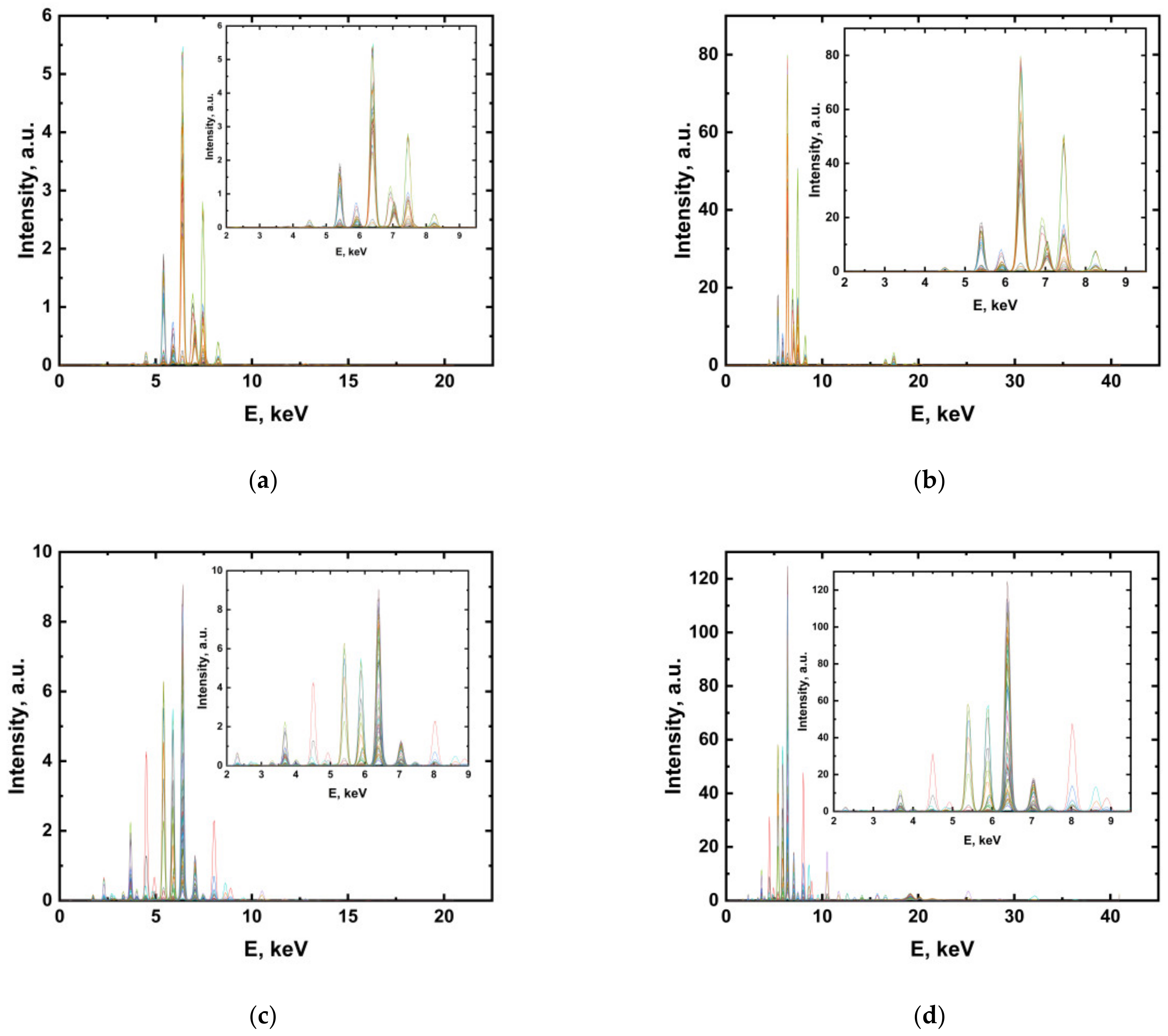
2.2. EDXRF Measurements

EDXRF spectra were acquired with Shimadzu EDX-800 (Shimadzu Corp., Kyoto, Japan) energy dispersive X-ray fluorescence spectrometer using an Rh anode X-ray tube. The measurements were performed with two different X-ray tube voltages: 15 and 50 kV. The lower voltage was employed to acquire the spectra of light elements (Na-Sc), and the higher one was used to analyze the heavier elements. The spectra registered with 15 kV voltage (XRF energies 0–20.48 keV) will be referred to hereafter as light channel. The spectra registered with 50 kV voltage (XRF energies 0–40.96 keV) will be referred to hereafter as heavy channel. The spectra accumulation time was 100 s. The measurements were performed in the air. The collimator spot size was 1 cm in diameter.

2.3. Data Processing

2.3.1. Fundamental Parameters Method

The fundamental parameters method [13] is based on the theoretical model of X-ray radiation interaction with matter in order to determine element content from XRF spectral intensities. The calculations employ such physical constants as attenuation coefficient, spectrum obtained from the X-ray tube itself, fluorescence yield for the element, branching ratio, and jump ratios. Thus, the application of FP does not require standard samples, only the known physical constants. This method only works well if the sample does not contain a considerable quantity of elements without pronounced X-ray fluorescence lines (typically, this is valid for light elements with atomic numbers below 11 in case of EDX spectrometers). Otherwise, the FP yields low accuracy of analysis. The FP calculations were performed in the proprietary Shimadzu software package for Shimadzu EDX-800.

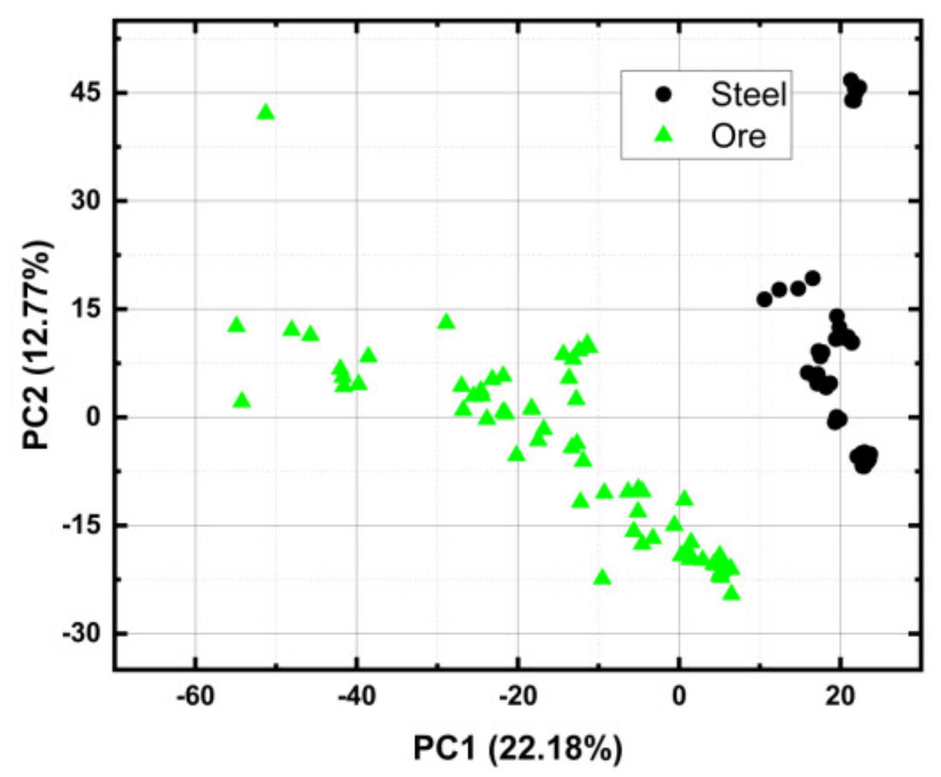
2.3.2. Exploratory Data Analysis

Principal component analysis (PCA) was employed for the data exploration. PCA is a common dimensionality reduction technique widely applied in chemometrics to study the similarity among the samples characterized by multiple variables [14].

2.3.3. IC-PLS

Influence coefficients-partial least squares (IC-PLS) is based on a combination of traditional IC method and PLS multivariate regression. The idea is to get rid of the limitation associated with IC that the number of parameters taken into account should be smaller than the number of available standard samples. For this purpose, a PLS algorithm is employed to calculate the regression coefficients in the IC equation instead of the traditional ordinary least squares procedure. At the first stage in IC-PLS, a matrix is constructed where the columns contain XRF signal intensities of analyzed and interfering elements, their products and ratios. Next, this matrix is employed for PLS modeling. The resulting model can be further applied for the quantification of elements in the new samples. A detailed explanation of the IC-PLS procedure can be found in [12]. In our study, the IC-PLS models were calculated in R environment [15] using an mdatools package [16].

2.3.4. KRLS

KRLS is a nonlinear regression method that develops ideas of generalized linear models. The main idea is to construct a function or a surface, which is then penalized for complexity via selecting one of many possible regression problem solutions with the help of kernels and the least squares problem. There are two explanations of KRLS: the “similarity-based” method and the “superposition of Gaussians” method.

The “similarity-based” method assumes that the data considered is i. i. d. and consists of yields y_i and a D-dimensional vector of covariate values x_i for i-th exemplar. Then a semi-defined positive and symmetric function is taken as the kernel k. This takes two numbers and produces a real value output y_i. In this article, the Gaussian kernel is used:

$$k\left(x_i{x}_j\right)=exp(\frac{{-\Vert x_i-x_j\Vert }^2}{{\sigma }^2})$$

(1)

where $\Vert x_i-x_j\Vert$ is the Euclidean distance between the covariate vectors x_i and x_j. The kernel bandwidth σ² is set to the number of dimensions in this work, though it can be varied [17]. The most important feature of this function is that it reaches its maximum of one only when x_i = x_j and gets closer to zero when the similarity between two vectors decreases.

The target function y = f(x) can be approximated by the equation:

$$f\left(x\right)={\displaystyle \sum }_i^N{c}_{i}k\left(x,x_i\right)$$

(2)

where $k\left(x,x_i\right)$ is the measurement of the similarity and c_i is the weight for each input pattern. Therefore, the main idea is to replace the linear combinations of functions of x_i with the similarity between a test point x and a fixed input pattern x_i. This should be a more appropriate point of view, as similar inputs should give similar outputs.

The “superposition of Gaussians” method supposes that an approximation function can be described with the help of Equation (2) where each $c_{i}k\left(x,x_i\right)$ is a different Gaussian curve centered around x_i and scaled by c_i. These Gaussians are summed up to give a resulting function, which is a more flexible approach than in linear methods as it allows describing nonlinear and nonadditive functions. For further understanding of KRLS we should rewrite (2) in a more convenient form:

$$y=Kc=\left[\begin{array}{cccc}k\left(x_1,x_1\right)& k\left(x_1,x_1\right)& \cdots & k\left(x_1,x_1\right)\\ k\left(x_1,x_1\right)& \ddots & & \\ ⋮& & & \\ k\left(x_1,x_1\right)& & & k\left(x_1,x_1\right)\end{array}\right]\begin{array}{c}{c}_1\\ c_1\\ \\ c_N\end{array}$$

(3)

Matrix K will be invertible, as it is positive, semidefinite, and symmetric. This means that there is a best solution to the linear system y = Kc which gives a function that provides the best fit for each data point.

To prevent overfitting, two more assumptions are made. The first is that the error of the function is counted as a squared loss so that the result could be easily interpreted as an expectation function. The second is that the complexity of the function is regularized by a parameter λ to perform a tradeoff between complexity and accuracy. This is needed because smoother functions tend to result in a better fitting due to the possible noise in the signal. Therefore, the Tikhonov regularization problem, which may help to find the best function fitting, in this case can be written as:

$$argmi{n}_{f\in H}{\displaystyle \sum }_i^N{\left(y_i-f\left(x_i\right)\right)}^2+\lambda {\Vert f\Vert }^2{}_H$$

(4)

where λ ∈ R⁺ and f is the sought function. ${\Vert f\Vert }^2{}_H$ is a L₂ norm in the reproducing kernel Hilbert spaces of functions associated with a particular choice of kernel.

To solve this problem, f(x) is replaced by Kc, and ${\Vert f\Vert }^2{}_H$ which is equal to ${\sum }_i{\sum }_j{c}_i{c}_{j}k\left(x_i{x}_j\right)$ is replaced by c^TKc. This results in:

$$c^{*}=argmi{n}_{c\in R^D}{\displaystyle \sum }_i^n{\left(y-Kc\right)}^T\left(y-Kc\right)+\lambda c^{T}Kc$$

(5)

Consequently, y* = Kc* gives the best-fitting function. It can also be shown that the solution can be found as:

$$c^{*}={\left(K+\lambda I\right)}^{-1}y$$

(6)

More details can be found in [18].

2.3.5. Quality Metrics for Models

In order to assess the quality of the models, Pearson r correlation coefficient and root mean square error (RMSE) values were employed. The RMSE was computed as follows:

$$\mathrm{RMSE}=\sqrt{\frac{{\sum }_{i=1}^n{\left(y_i-{\widehat{y}}_i\right)}^2}{n}}$$

(7)

where y is a certified value, $\widehat{y}$ is a predicted value, and n is the number of samples in the calibration (for RMSE of Calibration or RMSEC) or the test set (for RMSE of Prediction or RMSEP).

3. Results and Discussion

3.1. Exploratory Data Analysis

The acquired XRF spectra of the samples are presented in Figure 1. It can be seen that the visual appearance of the ore and steel samples spectra varies significantly due to the significant differences in chemical composition. In order to visualize all the samples simultaneously in a concise manner, we have applied PCA to the spectral data. The intensities obtained in light and heavy channels for each sample were merged prior to the analysis. The resulting PCA score plot is given in Figure 2. Two distinct clusters formed by the ore and steel samples correspondingly can be observed in this plot. This sample separation confirms the substantial difference in the spectra and the chemical composition and consequently in the expected matrix effects in the spectra.

Therefore, the calibration models built separately for ores and for steels will not be capable of accurate prediction in a cross manner: the calibration model for steels will not be able to handle ore samples properly, and vice versa. This is well illustrated by Figure 3, where “measured vs predicted” plots for the corresponding IC-PLS models are presented. Quantification of Al and Mn is considered as an example. Unacceptably poor accuracy of the predictions can be seen in all four plots. The cross-validated models built separately for the ores and for the steels for the quantification of Al and Mn are shown in Figure S1 (Supplementary Materials). Similar results were obtained for Si and Ti.

In attempting to construct a universal calibration model embracing both ore and steel samples, we have applied several quantitative modeling methods: FP, IC-PLS, and KRLS.

3.2. Splitting the Data into Calibration and Validation Sets

In order to ensure the comparability of the quantification models on the basis of various approaches, the data were split into calibration and test sets. This process was performed in three steps. First, the samples of steel/ore were sorted by the increase in concentration of the element of interest. Second, the two smallest and the two biggest concentrations of the element in steel/ore were taken to the calibration set (except for the Ti in steel samples, where only the smallest and the biggest concentrations were excluded, as there were only seven samples in total). Finally, every third sample from the sorted data was taken to the test set, while all the other samples were taken to the calibration set. The samples of steels and ores were merged together into a single calibration set and a single test set. This procedure allowed for comparatively uniform distribution of the concentration levels of the target elements in the calibration and test sets of both ores and steels. Thus, for each element different calibration and test sets containing both ore and steel samples were created (Table S3, Supplementary Materials).

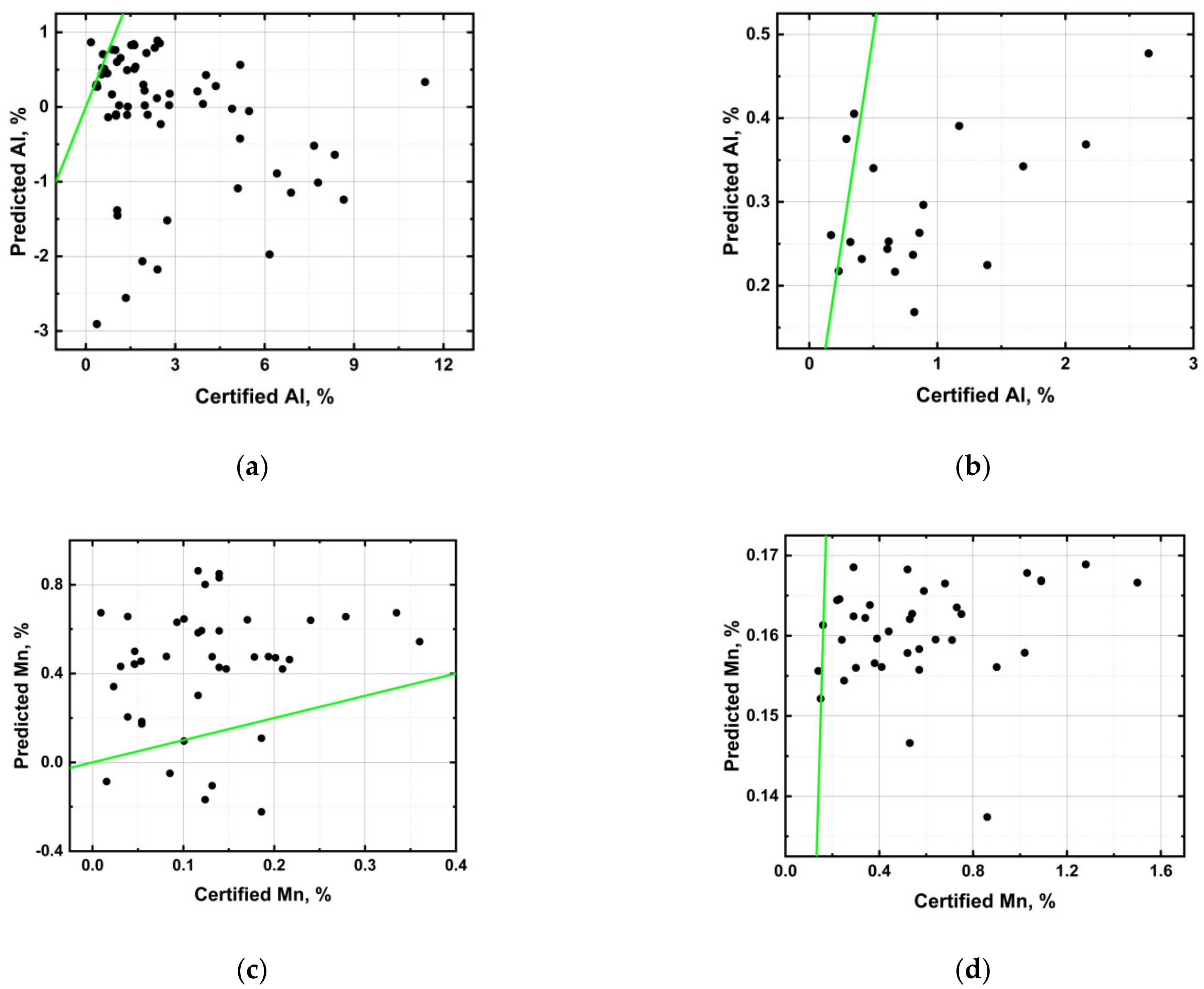
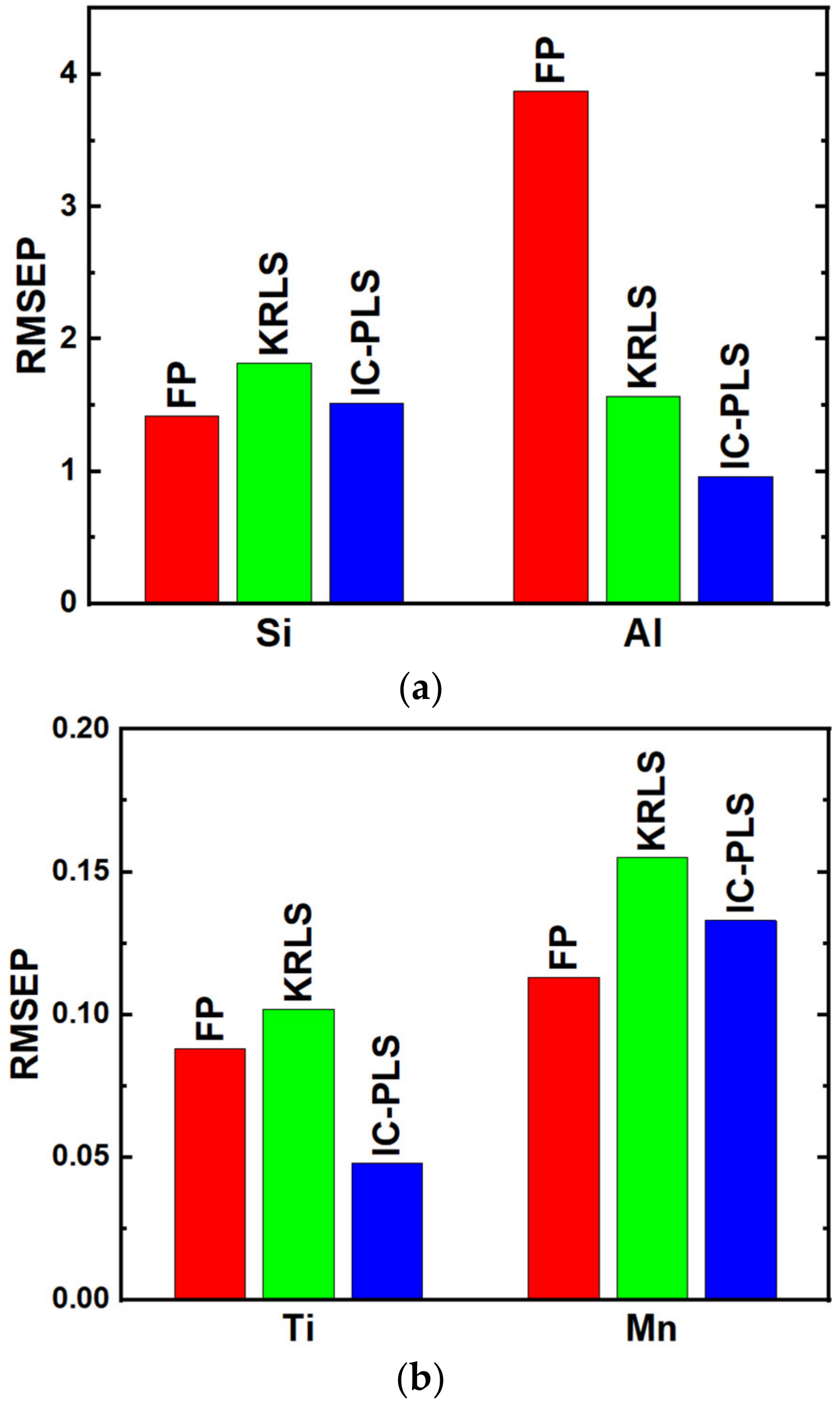
3.3. Multivariate Modeling for Universal Calibration

The acquired spectral data were employed for KRLS modeling to construct the calibration that could embrace the samples of both types. The spectral data matrix was cleaned from zero values for all the samples, as the KRLS input data may not contain missing or constant values [17]. The light (Na-Sc) and heavy (Ti-U) channel spectra were merged into a single data matrix with 3617 variables (wavelengths). Next, due to the uneven distribution of the target element content along the concentration ranges, only the samples with the concentration of the investigated elements below the threshold presented in Table S4 (Supplementary Materials) were taken into account. Otherwise, the contents that were significantly different from the rest of the samples will introduce a substantial bias into the regression modeling. The data were mean-centered and scaled with standard deviation prior to modeling.

The metrics of the obtained KRLS models for the quantification of Si, Al, Ti, and Mn in the framework of the universal model for ores and steels are given in Table 1 and Figure 4.

In the case of IC-PLS, the initial data matrix was composed of the X-ray fluorescence intensities of the K_α and K_β lines of all the elements presented in Table S1. The data from both spectral channels were employed. Then the columns containing ${\mathrm{I}}_{\mathrm{i}}^2$, I_i∗I_j, I_i/I_j and I_i²/I_j were added to the matrix.

The number of the latent variables (LV₁ in Table 1) was chosen according to the minimum of RMSE in full cross-validation (RMSECV). Next, variable selection was performed. Further VIP (variables important on projection) [19] scores were considered as a metric to eliminate insignificant variables. The threshold VIP score was chosen individually for each model in the course of the following procedure: the threshold VIP score value was varied from zero to the maximum value with the step of 5% from the maximum value; the optimal value was chosen according to the minimum of RMSECV. Finally, a new model based on the variables with a VIP score more than the threshold was built and the number of latent variables (LV₂ in Table 1) was once again chosen according to the minimum of RMSECV. The results are shown in

Table 2. The results of the algorithms’ implementation for different elements.

Element	Algorithm	Parameters	RMSEP	r
Si (0.03–36.00%)	FP		1.42	0.98
	KRLS	λ = 0.010	1.82	0.96
	IC-PLS	LV1 = 2, LV2 = 1	1.52	0.91
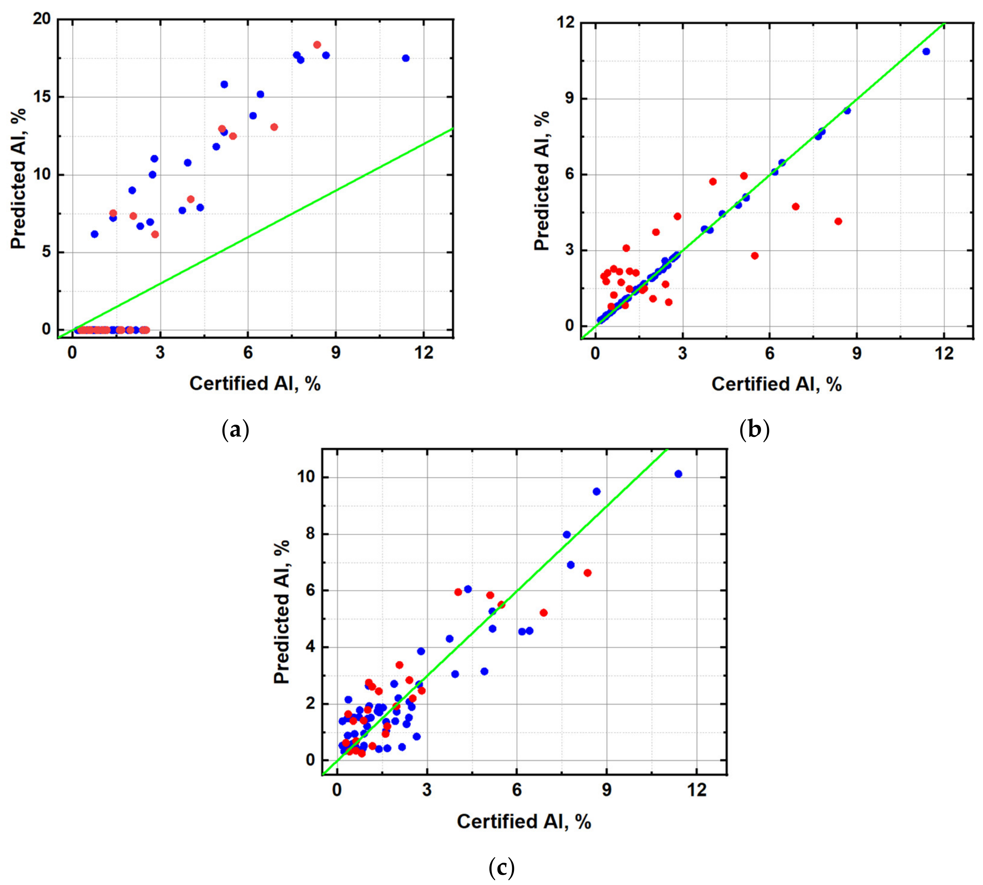
Al (0.17–11.40%)	FP		3.88	0.92
	KRLS	Λ = 0.023	1.57	0.68
	IC-PLS	LV1 = 2, LV2 = 2	0.96	0.90
Ti (0.01–1.00%)	FP		0.09	0.89
	KRLS	Λ = 0.002	0.10	0.65
	IC-PLS	LV1 = 2, LV2 = 1	0.05	0.94
Mn (0.01–1.75%)	FP		0.11	0.92
	KRLS	Λ = 0.001	0.16	0.83
	IC-PLS	LV1 = 5, LV2 = 2	0.13	0.88

and Figure 4. An example of predicted vs measured plot is shown for Al in Figure 5.

It can be seen that IC-PLS significantly outperforms traditional FP in terms of accuracy for predicting the content of Al (0.96% vs. 3.87%) and Ti (0.05% vs. 0.09%) and yields comparable results for Si and Mn. A possible explanation for this distribution of the results among the elements can be based on the nature of X-ray fluorescence signals. In case of Al, the energy of the fluorescence lines is low and the lines have low intensities compared to other studied elements. Thus, FP (which uses a single Al Kα line for concentration calculation) has to deal with noisy data. Both IC-PLS and KRLS take into account numerous intensities: Kα and Kβ from two channels for IC-PLS, and all the whole spectra for KRLS. In the case of Ti and Mn, FP performs better as it handles more intense lines in calculations. In the case of Si, the Kα line is also noisy as for Al; however, the content of Si in the samples is significantly higher and the signal-to-noise ratio is less critical here, thus FP yields an accuracy similar to IC-PLS here. KRLS has shown the worst performance with the lowest accuracy for the three elements and is only better than FP in the case of Al. Nevertheless, KRLS is able to handle nonlinear matrix effects and in general yields comparable accuracy with FP.

4. Conclusions

We have proposed a possible approach to handle the problem of universal calibration in XRF spectrometry. The samples with significantly different matrix elements cannot be effectively handled in the framework of a single calibration model, thus increasing the cost of XRF analysis due to the necessity of making individual calibrations for each sample type. The proposed approach is based on the application of the recently introduced IC-PLS method. We have demonstrated the potential of the IC-PLS approach for constructing universal calibration models embracing different types of samples in XRF. Using the example of ore and steel samples, we have shown that the quantification accuracy for certain elements increased up to four times compared to the conventional fundamental parameters method. The flexibility of the IC-PLS method in terms of possible inclusion of various number of spectral intensities, their ratios, and products implies a good promise for further development of universal calibration models in XRF.

References

- Taraškevičius, R.; Motiejūnaitė, J.; Zinkutė, R.; Eigminienė, A.; Gedminienė, L.; Stankevičius, Ž. Similarities and differences in geochemical distribution patterns in epiphytic lichens and topsoils from kindergarten grounds in Vilnius. J. Geochem. Explor. 2017, 183, 152–165. [Google Scholar] [CrossRef]
- Moreno-Santos, A.; Rios-Hurtado, J.C.; Flores-Villaseñor, S.E.; Esmeralda-Gomez, A.G.; Guevara-Chavez, J.Y.; Lara-Castillo, F.P.; Escalante-Ibarra, G.B. Hydroxyapatite Growth on Activated Carbon Surface for Methylene Blue Adsorption: Effect of Oxidation Time and CaSiO3 Addition on Hydrothermal Incubation. Appl. Sci. 2023, 13, 77. [Google Scholar] [CrossRef]
- Revenko, A.G. X-Ray Fluorescence Analysis in Pharmacology. In X-Ray Fluorescence in Biological Sciences; Singh, V.K., Kawai, J., Tripathi, D.K., Eds.; John Wiley & Sons, Ltd.: Hoboken, NJ, USA, 2022; pp. 475–488. [Google Scholar] [CrossRef]
- Ruschioni, G.; Micheletti, F.; Bonizzoni, L.; Orsilli, J.; Galli, A. FUXYA2020: A Low-Cost Homemade Portable EDXRF Spectrometer for Cultural Heritage Applications. Appl. Sci. 2022, 12, 1006. [Google Scholar] [CrossRef]
- Barago, N.; Pavoni, E.; Floreani, F.; Crosera, M.; Adami, G.; Lenaz, D.; Larese Filon, F.; Covelli, S. Portable X-ray Fluorescence (pXRF) as a Tool for Environmental Characterisation and Management of Mining Wastes: Benefits and Limits. Appl. Sci. 2022, 12, 12189. [Google Scholar] [CrossRef]
- Vanhoof, C.; Bacon, J.; Fittschen, U.; Vincze, L. Atomic spectrometry update: Review of advances in X-ray fluorescence spectrometry and its special applications. J. Anal. At. Spectrom. 2022, 37, 1761–1775. [Google Scholar] [CrossRef]
- Richard, M.R. Corrections for matrix effects in X-ray fluorescence analysis—A tutorial. Spectrochim. Acta B At. Spectrosc. 2006, 61, 759–777. [Google Scholar] [CrossRef]
- Wang, Y.; Zhao, X.; Kowalski, B.R. X-Ray Fluorescence Calibration with Partial Least-Squares. Appl. Spectrosc. 1990, 44, 998–1002. [Google Scholar] [CrossRef]
- Kaniu, M.I.; Angeyo, K.H.; Mwala, A.K.; Mangala, M.J. Direct rapid analysis of trace bioavailable soil macronutrients by chemometrics-assisted energy dispersive X-ray fluorescence and scattering spectrometry. Anal. Chim. Acta 2012, 729, 21–25. [Google Scholar] [CrossRef] [PubMed]
- Panchuk, V.; Yaroshenko, I.; Legin, A.; Semenov, V.; Kirsanov, D. Application of chemometric methods to XRF-data—A tutorial review. Anal. Chim. Acta 2018, 1040, 19–32. [Google Scholar] [CrossRef] [PubMed]
- Aidene, S.; Khaydukova, M.; Pashkova, M.; Chubarov, V.; Savinov, S.; Semenov, V.; Kirsanov, D.; Panchuk, V. Does chemometrics work for matrix effects correction in X-ray fluorescence analysis? Spectrochim. Acta B At. Spectrosc. 2021, 185, 106310. [Google Scholar] [CrossRef]
- Aidene, S.; Khaydukova, M.; Savinov, S.; Semenov, V.; Kirsanov, D.; Panchuk, V. Partial least squares assisted influence coefficients concept improves accuracy in X-ray fluorescence analysis. Spectrochim. Acta B At. Spectrosc. 2022, 193, 106452. [Google Scholar] [CrossRef]
- Kawai, J.; Yamasaki, K.; Tanaka, R. Fundamental Parameter Method in X-Ray Fluorescence Analysis. In Encyclopedia of Analytical Chemistry; Meyers, R.A., Ed.; John Wiley & Sons, Ltd.: Hoboken, NJ, USA, 2019; pp. 1–14. ISBN 9780470027318. [Google Scholar]
- Bro, R.; Smilde, A.K. Principal component analysis. Anal. Methods 2014, 6, 2812–2831. [Google Scholar] [CrossRef]
- R Core Team. R: A Language and Environment for Statistical Computing; R Foundation for Statistical Computing: Vienna, Austria, 2022; Available online: https://www.R-project.org/ (accessed on 22 April 2023).
- Kucheryavskiy, S. mdatools—R package for chemometrics. Chemometr. Intell. Lab. Syst. 2020, 198, 103937. [Google Scholar] [CrossRef]
- Jeremy, F.; Jens, H.; Chad, J.H. Kernel-Based Regularized Least Squares in R (KRLS) and Stata (krls). J. Stat. Softw. 2017, 79, 1–26. [Google Scholar] [CrossRef]
- Hainmueller, J.; Hazlett, C. Kernel Regularized Least Squares: Reducing Misspecification Bias with a Flexible and Interpretable Machine Learning Approach. Polit. Anal. 2014, 22, 143–168. [Google Scholar] [CrossRef]
- Andersen, C.M.; Bro, R. Variable selection in regression—A tutorial. J. Chemom. 2010, 24, 728–737. [Google Scholar] [CrossRef]