A Multidimensional Spectral Transformer with Channel-Wise Correlation for Hyperspectral Image Classification

Abstract

Convolutional neural networks (CNNs) have been developed as an effective strategy for hyperspectral image (HSI) classification. However, the lack of feature extraction by CNN networks is due to the network failing to effectively extract global features and poor capability in distinguishing between different feature categories that are similar. In order to solve these problems, this paper proposes a novel approach to hyperspectral image classification using a multidimensional spectral transformer with channel-wise correlation. The proposed method consists of two key components: an input mask and a channel correlation block. The input mask is used to extract relevant spectral information from hyperspectral images and discard irrelevant information, reducing the dimensionality of the input data and improving classification accuracy. The channel correlation block captures the correlations between different spectral channels and is integrated into the transformer network to improve the model’s discrimination power. The experimental results demonstrate that the proposed method achieves great performance with several benchmark hyperspectral image datasets. The input mask and channel correlation block effectively improve classification accuracy and reduce computational complexity.

1. Introduction

Hyperspectral imaging is a technique that acquires data from many narrow and contiguous spectral bands, enabling spectral signatures of various materials to be detected. Hyperspectral images, HSIs, produce data cubes that consist of a set of two-dimensional images, where each pixel contains the reflectance or radiance values at different wavelengths or bands. HSI classification is a process of assigning each pixel in an HSI to one of several predefined classes, which presents a challenging task due to the high-dimensional nature of hyperspectral data and the complexity of spectral signatures. HSI classification algorithms are designed to extract useful information from the hyperspectral data and map this information to the predefined classes. This process involves the use of mathematical algorithms and statistical techniques to analyse the spectral information contained in each pixel.

HSI classification algorithms have a wide range of applications, including mineral and oil exploration and environmental monitoring [1,2,3,4,5]. In mineral and oil exploration [6], hyperspectral imaging can be used to identify the presence of specific minerals or hydrocarbons based on their unique spectral signatures. Environmental monitoring applications include the detection of pollutants and the mapping of vegetation types [7,8].

Many algorithms have been developed for HSI classification, including supervised, unsupervised, and hybrid approaches. Supervised algorithms rely on prior knowledge about the spectral properties of the target of interest, and use this information to train a classification model. The most common supervised classification algorithm employed in hyperspectral imaging is the maximum likelihood classifier [9]. This algorithm assumes that the spectral response of each target class is normally distributed, and calculates the probability that each pixel belongs to each class. The pixel is then classified to the class with the highest probability. Other supervised classification algorithms include support vector machines [10], decision trees [11], and artificial neural networks [12]. Unsupervised classification algorithms include clustering algorithms such as k-means [13], hierarchical clustering [14], and self-organizing maps [15,16]. These algorithms group pixels into clusters based on their spectral similarity, without any prior knowledge of the target classes. The resulting clusters can then be labelled and classified based on their spectral properties. Hybrid algorithms combine the strengths of both supervised and unsupervised approaches. For example, a hybrid algorithm might use an unsupervised clustering algorithm to group pixels into clusters, and then use a supervised algorithm to assign labels to the clusters based on prior knowledge of the target classes.

The traditional algorithms mentioned above mostly focus on classifying different extracted features [17]. With the development of deep learning research [18], HSI classification methods have gradually shifted to extracting and classifying high-level deep features. Convolutional neural network (CNN)-based methods are widely used due to their end-to-end architecture and good classification properties. These architectures consist of multiple layers of convolutional and pooling operations, which are used to learn hierarchical features from the input data. The classifier in the end learns to classify each pixel based on the features learned from the input data, and the final output of the algorithm is a classification map that assigns a label or class to each pixel in the HSI.

The deep belief network (DBN) [19], stacked autoencoder (SAE) [20], and recurrent neural network (RNN) [21] treat each HSI pixel as independent spectral signatures for deep learning networks, which cannot extract sufficient information. Chen et al. [22] first designed a CNN framework extracting simple deep features from HSIs. To extract more convincing features, researchers developed the backbone for deep learning networks, such as GoogleNet [23] and Resnet [24], with skip architectures. Zhong et al. [25] proposed the framework of a 3D CNN with the residual block from Resnet and obtained deeper features for classification. One recently proposed HSI classification algorithm is the residual attention network (RAN), proposed by Wang et al. [26]. RAN is a deep-learning-based algorithm that integrates residual connections and attention mechanisms to improve the classification performance. The residual connections help to alleviate the vanishing gradient problem and enable the network to learn more complex features, while the attention mechanism helps to focus on discriminative features and suppress noisy ones. Experimental results on several benchmark hyperspectral datasets demonstrated that RAN outperforms many state-of-the-art methods in terms of classification accuracy. The CNN-based HSI classification algorithms have been shown to be effective at achieving high levels of classification accuracy, particularly when large amounts of labelled training data are available.

With the development of natural language processing (NLP) technology, the transformer architecture shows a strong feature extraction ability, especially when applied to the vision tasks. Vision transformer [27] has been applied to computer vision (CV) and shown exciting results. He et al. [28] designed a BERT-like architecture, which flattens the HSI cube as a sequence of the transformer input. Hong et al. [29] proposed the SpectralFormer network, which learns information from neighbouring bands. However, the current transformer-based methods for HSI classification introduce feature inconsistencies generated by a large number of differences between different bands when directly inputting samples into adjacent bands as a sequence, resulting in insufficient feature-extraction capabilities. Furthermore, the network fails to consider the correlation between the feature channels when modelling the input vector.

We proposed a multidimensional spectral transformer with channel-wise correlation (MSTCC) to combine neighbouring band features and feed them to vectors used to classify their differences. The main contributions of this paper are as follows:

• To overcome difficulties that arise when extracting global features with a CNN, we proposed a transformer-based network architecture to better extract long-range relationship features of cube bands from HSIs;
• To better combine the related features between bands of different dimensions, we proposed a channel-related feature extraction method;
• Combining all the above-mentioned points, we proposed a new method for HSI classification. We also validated the proposed model using several comparison methods, revealing that it achieved great results on the studied datasets.

2. Materials

2.1. The Dataset

To demonstrate the performance of our proposed network, we evaluated it on three datasets, Indian Pines (IP), Pavia University (PU), and Pavia centre (PC). We divided them into training and testing sets and introduce them below. IP was set by the airborne visible/infrared imaging spectrometer (AVIRIS) sensor over north-western Indiana, USA. The spatial resolution of the dataset is about 20 m per pixel and the images consist of 145 × 145 pixels with 224 bands ranging from 0.4 to 2.5 μm. In our experiments, the dataset had 200 spectral bands after removing the water absorption bands, covering 16 land features, as is shown in

Table 1. Number of selected pixels from the IP dataset.

Class No.	Class Name	Training	Testing
1	Corn Notill	50	1384
2	Corn Mintill	50	784
3	Corn	50	184
4	Grass Pasture	50	447
5	Grass Trees	50	697
6	Hay Windrowed	50	439
7	Soybean Notill	50	918
8	Soybean Mintill	50	2418
9	Soybean Clean	50	564
10	Wheat	50	162
11	Woods	50	1244
12	Buildings Grass Trees Drivers	50	330
13	Stone Steel Towers	50	45
14	Alfalfa	15	39
15	Grass Pasture Mowed	15	11
16	Oats	15	5
	Total	695	9671

.

PU was collected by the reflective optics system imaging spectrometer (ROSIS) sensor. The images consist of 610 × 340 pixels with a 1.3 m spatial resolution and 103 spectral bands in the wavelength range 0.38 to 0.86 μm. The dataset covers nine classes of ground objects, as shown in

Table 2. Number of selected pixels from the PU dataset.

Class No.	Class Name	Training	Testing
1	Asphalt	50	6802
2	Meadows	50	18,636
3	Gravel	50	2157
4	Trees	50	3386
5	Metal sheets	50	1328
6	Bare Soil	50	5054
7	Bitumen	50	1306
8	Blocking Bricks	50	3828
9	Shadows	50	976
	Total	450	43,473

.

The PC images were captured by the ROSIS sensor over an urban area surrounding the centre of Pavia, Italy. The dataset consists of 1096 × 492 pixels with 103 spectral bands, from which 12 noisy bands were removed. The dataset contained nine classes of ground objects, as shown in

Table 3. Number of selected pixels from the PC dataset.

Class No.	Class Name	Training	Testing
1	Water	50	65,228
2	Trees	50	6457
3	Meadows	50	2841
4	Blocking Bricks	50	2102
5	Bare Soil	50	6499
6	Asphalt	50	7475
7	Bitumen	50	7507
8	Tiles	50	3072
9	Shadows	50	2115
	Total	450	103,296

.

2.2. Evaluation

To evaluate our proposed method with others and demonstrate its classification performance, we selected the overall accuracy (OA) and Kappa coefficient as the classification indexes. The OA computes the percentage of test pixels which are correctly classified. The Kappa coefficient collects pixels correctly classified by the number of pure expected agreements by change and shows the percentage of them. The performance of these two methods is positively correlated with the index value.

2.3. Experiment Implementation

Our proposed network is based on Pytorch backend and performed on a desktop computer with a NVIDIA GTX3090 GPU.We selected three typical CNN-based methods, including CNN-2D, CNN-3D, and FCN-ELM [30], and one transformer-based method, SpectralFormer [29], to compare with our work. For the fairness of the comparison, our proposed MSTCC method and the comparison methods adopted the same image pre-processing and hyperparameter network settings. We set the spatial size of input image cube as 27 × 27 and the batch size of training as 32.

3. Our Methods

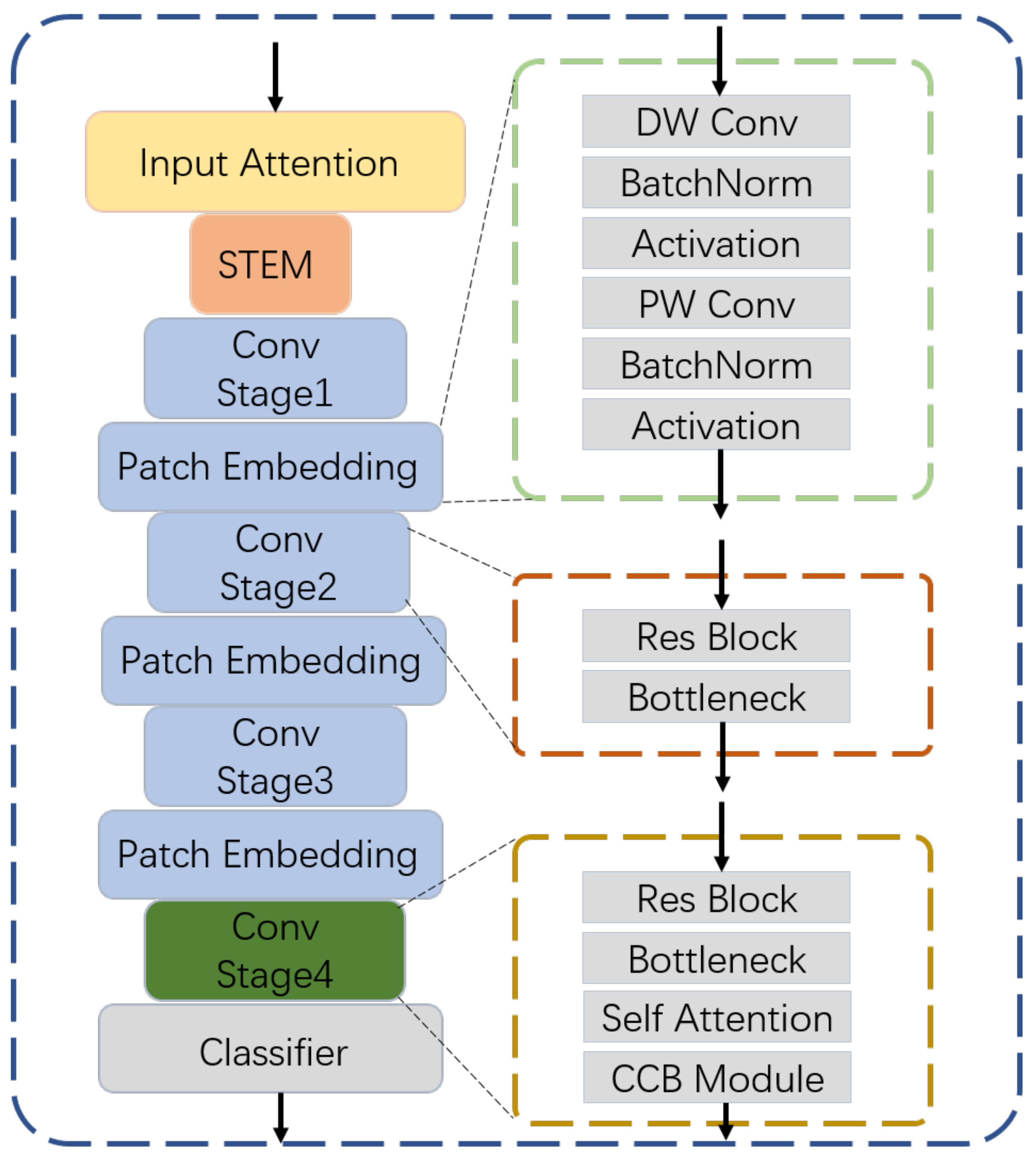
Our MSTCC is based on the transformer architecture with a well-designed CCB (channel correlation block) module. We did not manually set the fixed region, instead the network searches pixels via an attention-based method which preserves the feature stability of the region. The overall framework of the MSTCC is shown in Figure 1.

Our architecture is based on the transformer methods, which contain patch embedding modules and convolutional modules for feature extraction. The patch embedding module consists of depth-wise convolution layers, point-wise convolution, batch normalization layers and activation layers. The depth-wise convolution layers and the point-wise convolution layers are used to increase feature latitudes and reduce computational complexity. The activation layers in our method is the ReLU activation, which achieved great results in classification tasks.

3.1. Input Mask for Training

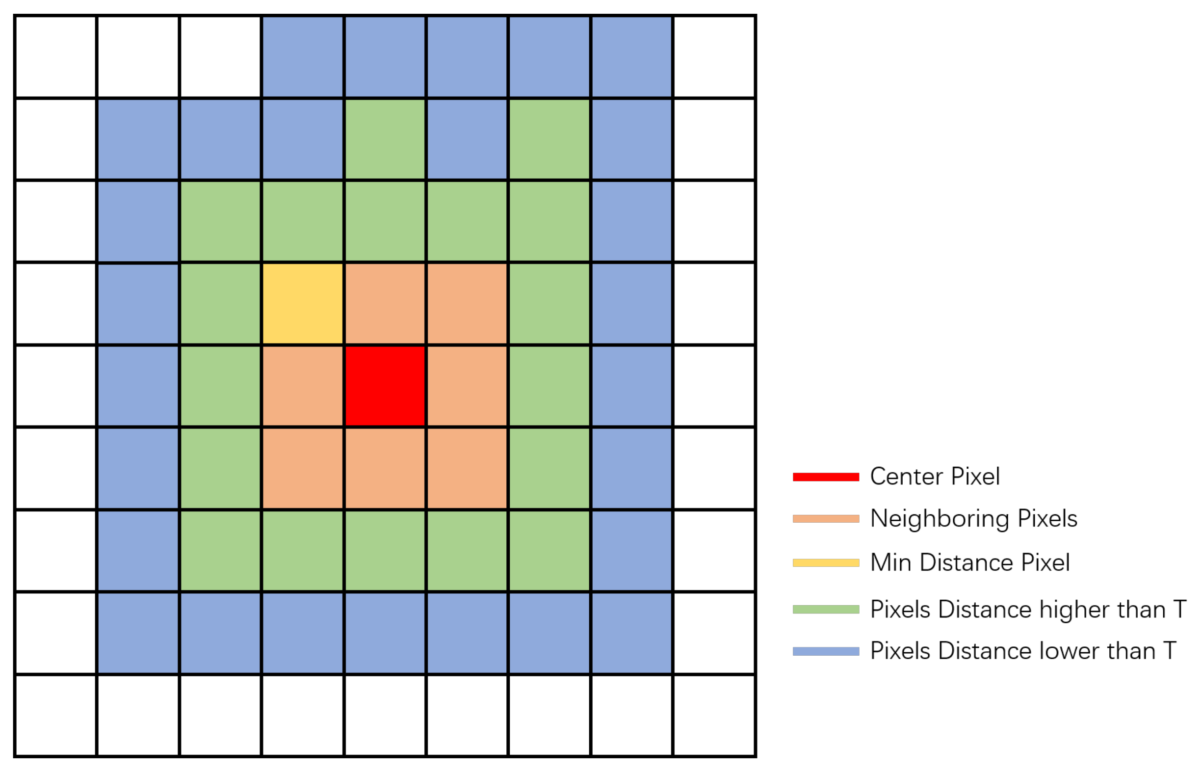
The relationship between adjacent pixels is different, so the length of the image cube as the input should change accordingly to improve the effectiveness of feature extraction. We suppose that the input dataset is $X=\{x_1,x_2,\dots ,x_n\},n=H\times W,x_i\in {\mathcal{R}}^{C\times 1}$.

For each $x_i$ ($i^{th}$ pixel in the image), we calculated the correlation distance between it and surrounding pixels, taking a minimum of eight adjacent pixels as the threshold $T_i$, recording all correlation distances as $D=\{di{s}_1,di{s}_2,\dots di{s}_8\}$. We calculated the correlation between each point and the centre pixel extending from the centre along the horizontal and vertical directions, and added the distance to D until its value was less than $T_i$.

All similar distances in D were normalized as coefficients of the corresponding pixel points, where the coefficient for pixel i was computed via the following equation:

$${\mathcal{S}}_{i,j}=\frac{e^{di{s}_{i,j}}}{{\sum }_{k=1}^N{e}^{di{s}_{i,k}}},$$

(1)

where i and j indicate the indices of the centre pixel and its correlated pixel for $j\in \left[1,N\right]$. We extracted the feature vectors by two $1\times 1$ convolutional layers, $W_{\theta }$ and $W\eta$, which were used to transform the multidimensional features to one dimension with the coefficient $S_{i,j}$ for each pixel. In our experiments, the parameters of these two layers were learnt from training. The correlation between the two pixels was computed using the Gaussian distance. This attention-based method is shown in Figure 2.

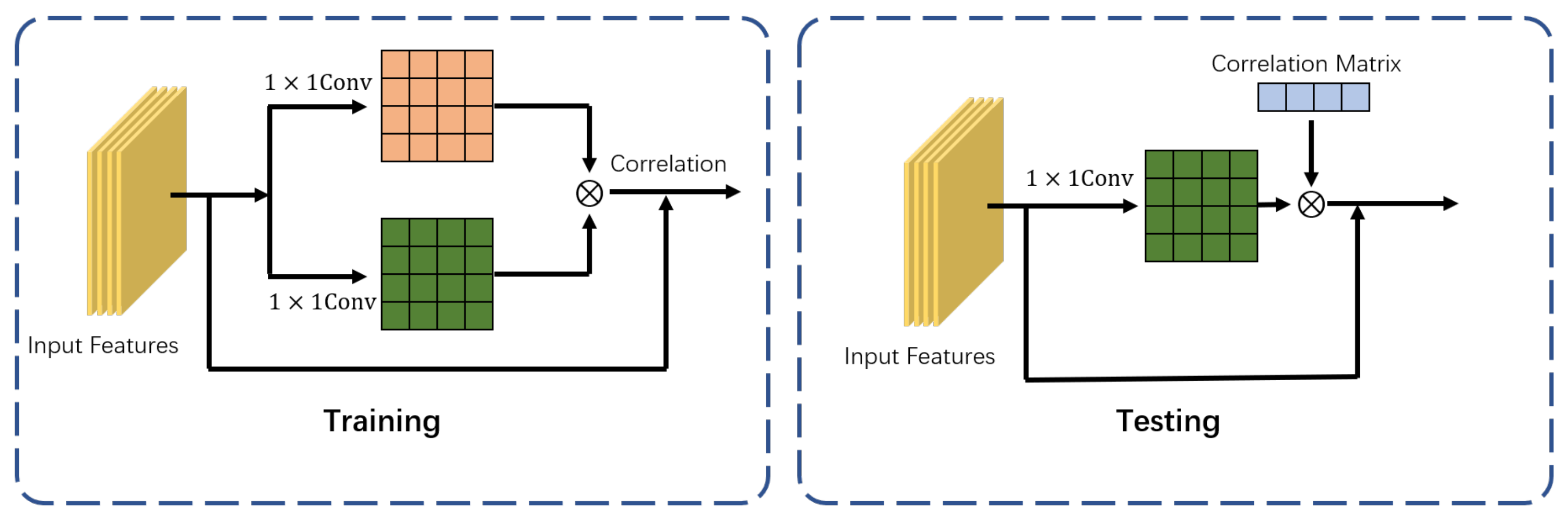
3.2. Channel Correlation Block

In view of the poor ability of network classifiers to identify similar features, we proposed a channel-wise method to extract the features by designing a channel correlation module. The module architecture is shown in Figure 3. When extracting features into the classifier during training, the channel correlation matrix converts the feature information as a learnable parameter and adds it to the self-attention module of the fourth stage.

4. Results

4.1. Ablation Study

To verify the effectiveness of our proposed network structure components, we conducted ablation experiments on three datasets. We chose the ViT-based HSI classification method as the baseline, and only compared the input mask modules of the methods, the CCB module, and two modules at the same time in

Table 4. Classification accuracy (%) of the two proposed components for the ablation study with the OA on the IP dataset.

	IP	PU	PC
Baseline	89.3	92.5	95.8
Input Mask	89.9	91.8	96.5
CCB Module	91.7	94.6	96.0
Input Mask + CCB Module	91.9	94.9	96.7

. The accuracy of the method with the input mask was slightly improved on the two datasets, IP and PC. However, its accuracy decreased by about $0.7\%$ on the PU dataset. The accuracy of the method with the CCB module improved significantly when using the two datasets, IP and PU, and slightly improved on the PC dataset. The combination of the two modules improved when compared with the baseline and the two modules alone, indicating that the two modules were not coupled to each other and can jointly improve the feature extraction ability of the model at different levels, thus improving the classification accuracy.

4.2. Comparison with Other Methods

To demonstrate the performance of our proposed MSTCC, we selected four methods for qualitative comparison on three datasets and quantitative comparison on two datasets. The hyperparameter settings were the same as those previously used. The learning rate was initialized at $1\times {10}^{-4}$ and decayed by a factor of 0.9 after every 100 epochs. The total epoch on the datasets was 500.

The first experiment was reported on the IP dataset. We roughly set 50 labelled pixels in each land-cover category for training and the rest for testing. The OA and Kappa coefficient are shown in

Table 5. Classification accuracy (%) of different methods with their OA and Kappa coefficients on the IP dataset.

Class	CNN-2D	CNN-3D	FCN-ELM	SpectralFormer	MSTCC (Ours)
1	83.1	81.7	60.1	70.5	84.2
2	74.7	86.5	88.4	82.1	80.7
3	94.2	93.6	76.9	90.2	88.6
4	81.4	80.6	89.1	95.6	97.1
5	89.5	83.4	90.2	85.1	96.5
6	88.2	97.3	93.2	96.9	95.7
7	81.9	88.6	75.7	82.3	89.1
8	87.8	86.9	97.7	74.7	97.8
9	79.3	83.2	63.2	73.6	90.2
10	98.6	94.1	85.7	99.2	99.7
11	95.9	94.9	84.3	91.5	93.4
12	91.8	89.7	89.5	79.8	90.4
13	59.7	72.6	96.1	99.6	96.5
14	78.1	44.8	95.8	79.2	97.8
15	46.4	26.7	59.3	59.2	68.3
16	65.1	23.8	96.5	63.7	97.6
OA	85.6	86.7	87.9	90.1	91.9
Kappa	84.1	84.6	87.7	89.4	90.2

. Our proposed method achieved the best performance compared to the other four methods. In particular, the MSTCC demonstrated a $5.2\%$ increase in OA and a $5.6\%$ increase in the Kappa coefficient compared with CNN-3D, which performed better than CNN-2D. Furthermore, the performance of the MSTCC was also better than that of the FCN-ELM, which performed well on the IP dataset as a CNN-based method. For the transformer-based methods, SpectralFormer and our proposed method achieved better accuracy than the CNN methods, where the former improved by $1.8\%$ OA and $0.8\%$ Kappa coefficient.

The second experiment evaluated the performance of the compared methods on the PU dataset, shown in

Table 6. Classification accuracy(%) of different methods with their OA and Kappa coefficients on the PU dataset.

Class	CNN-2D	CNN-3D	FCN-ELM	SpectralFormer	MSTCC (Ours)
1	89.6	93.1	90.4	91.6	87.6
2	93.2	96.4	97.1	93.8	98.5
3	78.1	83.9	78.9	89.7	91.3
4	83.7	83.5	89.2	88.9	89.7
5	86.2	90.1	93.7	94.7	93.5
6	85.2	93.7	86.8	94.1	95.6
7	81.9	86.8	77.9	88.2	83.2
8	88.6	90.4	93.4	79.8	96.4
9	84.4	67.2	92.6	86.3	93.2
OA	89.3	93.1	93.2	93.4	94.9
Kappa	85.6	90.5	91.3	91.2	92.1

. Our MSTCC method performed better than all the state-of-the-art methods. It was $1.5\%$ higher for OA with a $0.9\%$ higher Kappa coefficient than the SpectralFormer, and much higher than the other CNN-based methods. Therefore, it can be inferred that our method more effectively identified all the land-cover categories compared to the CNN-based methods. The proposed components can thus increase the accuracy of the base transformer classifier.

The third experiment’s results are shown in

Table 7. Classification accuracy(%) of different methods with their OA and Kappa coefficients on the PC dataset.

Class	CNN-2D	CNN-3D	FCN-ELM	SpectralFormer	MSTCC (Ours)
1	99.9	99.9	99.6	99.9	99.9
2	63.1	87.3	89.3	89.6	89.6
3	52.9	56.1	57.8	59.2	56.7
4	57.2	42.7	49.2	58.3	67.2
5	73.8	86.2	88.1	89.5	79.1
6	78.9	81.3	80.6	79.2	86.4
7	89.1	90.3	93.5	94.2	94.7
8	96.7	98.7	99.3	98.6	99.7
9	67.2	81.9	79.5	83.5	86.9
OA	91.8	94.8	95.4	96.1	96.7
Kappa	88.9	92.5	93.6	94.3	95.2

. Similar to the above two datasets, our method achieved the best performance on the PC dataset. Both the OA and Kappa coefficient were higher than $95\%$. Each class of the dataset was more accurately classified than the other CNN-based methods. The OA result was $0.6\%$ higher than the SpectralFormer, while the Kappa coefficient was $0.9\%$.

For the qualitative evaluation, we selected all the methods and visualised them on the IP dataset and PU dataset, as shown in Figure 4 and Figure 5. The results of our MSTCC methods are smooth and clear, performing better than other methods, especially the CNN-based methods. Thus, we can deduce that CCB’s proficient capacity to capture distinctive attention features contributes to the successful classification of mixed pixels located near class borders. The visualization results of the CCB module and input mask have a finer appearance than the others, especially on the pixel boundary.

5. Discussion

In this work, we proposed two aspects for HSI classification:

1.

To extract HSI image features, and strengthen the connection between adjacent pixels, we proposed a transformer-based architecture with a mask input. This improved network performance in training.

2.

To enhance the classifier’s ability to discriminate between the input features, we proposed the channel correlation block (CCB) module to enhance its ability to distinguish between similar features.

Our proposed method shows that the transformer-based model can better extract global features than the CNN model, rather than just localized features. The correlation between different channels can better help the model distinguish HSI categories. We set up three CNN-based methods and one transformer-based method to conduct comparative experiments with our transformer-based method. The OA and Kappa coefficients of the latter two groups were higher than the former on the three datasets, proving the effectiveness of global feature classification.

For the two modules proposed, ablation experiments were set up to analyse their effectiveness. It can be seen from the OA and Kappa indicators that the CCB module performed better than the input mask. This shows that the correlation of deep features can more effectively distinguish features and improve the discriminative ability of the classifiers. The input mask, being a priori information for feature extraction, can reduce invalid information extraction in model training and improve the classification accuracy. These two methods improve the feature extraction ability of the model at different levels. The two components can be added to the model at the same time, and they achieved the best accuracy on three datasets, outperforming in the other individual settings in the ablation experiment.

For the input mask component, we found that the pixel correlation of each pixel in its various directions decreased significantly with distance. The correlation between features exceeding a certain distance threshold and the features of the point pixel was low, so the mask input aided the model to focus on the feature information of each pixel to improve feature discrimination.

Regarding the channel correlation block component, we found that in the last stage of the transformer architecture, the self-attention module was used to strengthen the mutual discrimination between pixel features. The similarity between features can be computed, together with the self-attention module, to provide high-quality features for the classifier.

As a method of processing at the beginning, the input mask received low-level features with spatial sparsity, resulting in instability in the different inputs. For example, compared with the baseline on the PU dataset, the classification accuracy decreased slightly for the model with the input mask. However, in general, adding the mask to an image effectively focussed in on high-value feature information and improved the accuracy of model classification. In contrast, the CCB module with deep features and dense information increased the similar feature extraction ability of the classifier.

6. Conclusions

We proposed a new transformer-based HSI classification method, improving the feature extraction ability of the model for HSI by adding an input mask and a correlation coefficient to the attention module. The proposed new method was evaluated against other reference methods on three experimental datasets, outperforming all studied competitors. Furthermore, from the ablation experiment, the two proposed modules effectively improved the feature extraction ability of the model, obtaining a better classification performance. In the future, the proposed model needs to be improved in terms of computational efficiency and optimization of its processing speed.

References

1. Camps-Valls, G.; Tuia, D.; Bruzzone, L.; Benediktsson, J.A. Advances in hyperspectral image classification: Earth monitoring with statistical learning methods. IEEE Signal Process. Mag. 2013, 31, 45–54. [Google Scholar] [CrossRef]
2. Ghiyamat, A.; Shafri, H.Z. A review on hyperspectral remote sensing for homogeneous and heterogeneous forest biodiversity assessment. Int. J. Remote Sens. 2010, 31, 1837–1856. [Google Scholar] [CrossRef]
3. Lu, G.; Fei, B. Medical hyperspectral imaging: A review. J. Biomed. Opt. 2014, 19, 010901. [Google Scholar] [CrossRef] [PubMed]
4. Ghamisi, P.; Dalla Mura, M.; Benediktsson, J.A. A survey on spectral–spatial classification techniques based on attribute profiles. IEEE Trans. Geosci. Remote Sens. 2014, 53, 2335–2353. [Google Scholar] [CrossRef]
5. Sun, H.; Zheng, X.; Lu, X.; Wu, S. Spectral–spatial attention network for hyperspectral image classification. IEEE Trans. Geosci. Remote Sens. 2019, 58, 3232–3245. [Google Scholar] [CrossRef]
6. Kruse, F.A.; Boardman, J.W.; Huntington, J.F. Comparison of airborne hyperspectral data and EO-1 Hyperion for mineral mapping. IEEE Trans. Geosci. Remote Sens. 2003, 41, 1388–1400. [Google Scholar] [CrossRef]
7. Stuart, M.B.; McGonigle, A.J.; Willmott, J.R. Hyperspectral imaging in environmental monitoring: A review of recent developments and technological advances in compact field deployable systems. Sensors 2019, 19, 3071. [Google Scholar] [CrossRef]
8. Briottet, X.; Boucher, Y.; Dimmeler, A.; Malaplate, A.; Cini, A.; Diani, M.; Bekman, H.; Schwering, P.; Skauli, T.; Kasen, I.; et al. Military applications of hyperspectral imagery. In Targets and Backgrounds XII: Characterization and Representation; SPIE: Bellingham, WA, USA, 2006; Volume 6239, pp. 82–89. [Google Scholar]
9. Richards, J.A.; Jia, X. Using suitable neighbors to augment the training set in hyperspectral maximum likelihood classification. IEEE Geosci. Remote Sens. Lett. 2008, 5, 774–777. [Google Scholar] [CrossRef]
10. Marconcini, M.; Camps-Valls, G.; Bruzzone, L. A composite semisupervised SVM for classification of hyperspectral images. IEEE Geosci. Remote Sens. Lett. 2009, 6, 234–238. [Google Scholar] [CrossRef]
11. Goel, P.K.; Prasher, S.O.; Patel, R.M.; Landry, J.A.; Bonnell, R.; Viau, A.A. Classification of hyperspectral data by decision trees and artificial neural networks to identify weed stress and nitrogen status of corn. Comput. Electron. Agric. 2003, 39, 67–93. [Google Scholar] [CrossRef]
12. Zherebtsov, E.; Dremin, V.; Popov, A.; Doronin, A.; Kurakina, D.; Kirillin, M.; Meglinski, I.; Bykov, A. Hyperspectral imaging of human skin aided by artificial neural networks. Biomed. Opt. Express 2019, 10, 3545–3559. [Google Scholar] [CrossRef] [PubMed]
13. Blanzieri, E.; Melgani, F. Nearest neighbor classification of remote sensing images with the maximal margin principle. IEEE Trans. Geosci. Remote Sens. 2008, 46, 1804–1811. [Google Scholar] [CrossRef]
14. Gillis, N.; Kuang, D.; Park, H. Hierarchical clustering of hyperspectral images using rank-two nonnegative matrix factorization. IEEE Trans. Geosci. Remote Sens. 2014, 53, 2066–2078. [Google Scholar] [CrossRef]
15. Riese, F.M.; Keller, S.; Hinz, S. Supervised and semi-supervised self-organizing maps for regression and classification focusing on hyperspectral data. Remote Sens. 2019, 12, 7. [Google Scholar] [CrossRef]
16. Jain, D.K.; Dubey, S.B.; Choubey, R.K.; Sinhal, A.; Arjaria, S.K.; Jain, A.; Wang, H. An approach for hyperspectral image classification by optimizing SVM using self organizing map. J. Comput. Sci. 2018, 25, 252–259. [Google Scholar] [CrossRef]
17. Jia, X.; Kuo, B.C.; Crawford, M.M. Feature mining for hyperspectral image classification. Proc. IEEE 2013, 101, 676–697. [Google Scholar] [CrossRef]
18. LeCun, Y.; Bengio, Y.; Hinton, G. Deep learning. Nature 2015, 521, 436–444. [Google Scholar] [CrossRef] [PubMed]
19. Chen, Y.; Zhao, X.; Jia, X. Spectral–spatial classification of hyperspectral data based on deep belief network. IEEE J. Sel. Top. Appl. Earth Obs. Remote Sens. 2015, 8, 2381–2392. [Google Scholar] [CrossRef]
20. Chen, Y.; Lin, Z.; Zhao, X.; Wang, G.; Gu, Y. Deep learning-based classification of hyperspectral data. IEEE J. Sel. Top. Appl. Earth Obs. Remote Sens. 2014, 7, 2094–2107. [Google Scholar] [CrossRef]
21. Mou, L.; Ghamisi, P.; Zhu, X.X. Deep recurrent neural networks for hyperspectral image classification. IEEE Trans. Geosci. Remote Sens. 2017, 55, 3639–3655. [Google Scholar] [CrossRef]
22. Chen, Y.; Jiang, H.; Li, C.; Jia, X.; Ghamisi, P. Deep feature extraction and classification of hyperspectral images based on convolutional neural networks. IEEE Trans. Geosci. Remote Sens. 2016, 54, 6232–6251. [Google Scholar] [CrossRef]
23. Szegedy, C.; Liu, W.; Jia, Y.; Sermanet, P.; Reed, S.; Anguelov, D.; Erhan, D.; Vanhoucke, V.; Rabinovich, A. Going deeper with convolutions. In Proceedings of the IEEE Conference on Computer Vision and Pattern Recognition, Boston, MA, USA, 7–12 June 2015; pp. 1–9. [Google Scholar]
24. He, K.; Zhang, X.; Ren, S.; Sun, J. Deep residual learning for image recognition. In Proceedings of the IEEE Conference on Computer Vision and Pattern Recognition, Las Vegas, NV, USA, 27–30 June 2016; pp. 770–778. [Google Scholar]
25. Zhong, Z.; Li, J.; Luo, Z.; Chapman, M. Spectral–spatial residual network for hyperspectral image classification: A 3-D deep learning framework. IEEE Trans. Geosci. Remote Sens. 2017, 56, 847–858. [Google Scholar] [CrossRef]
26. Wang, F.; Jiang, M.; Qian, C.; Yang, S.; Li, C.; Zhang, H.; Wang, X.; Tang, X. Residual attention network for image classification. In Proceedings of the IEEE Conference on Computer Vision and Pattern Recognition, Honolulu, HI, USA, 21–26 July 2017; pp. 3156–3164. [Google Scholar]
27. Dosovitskiy, A.; Beyer, L.; Kolesnikov, A.; Weissenborn, D.; Zhai, X.; Unterthiner, T.; Dehghani, M.; Minderer, M.; Heigold, G.; Gelly, S.; et al. An image is worth 16 × 16 words: Transformers for image recognition at scale. arXiv 2020, arXiv:2010.11929. [Google Scholar]
28. He, J.; Zhao, L.; Yang, H.; Zhang, M.; Li, W. HSI-BERT: Hyperspectral image classification using the bidirectional encoder representation from transformers. IEEE Trans. Geosci. Remote Sens. 2019, 58, 165–178. [Google Scholar] [CrossRef]
29. Hong, D.; Han, Z.; Yao, J.; Gao, L.; Zhang, B.; Plaza, A.; Chanussot, J. SpectralFormer: Rethinking hyperspectral image classification with transformers. IEEE Trans. Geosci. Remote Sens. 2021, 60, 1–15. [Google Scholar] [CrossRef]
30. Li, J.; Zhao, X.; Li, Y.; Du, Q.; Xi, B.; Hu, J. Classification of hyperspectral imagery using a new fully convolutional neural network. IEEE Geosci. Remote Sens. Lett. 2018, 15, 292–296. [Google Scholar] [CrossRef]
Figure 1. Architecture of our proposed MSTCC.
Applsci 13 05482 g001
Figure 2. Input mask to extract features. Each pixel generated its own mask with normalized corrections.
Applsci 13 05482 g002
Figure 3. Channel correlation block-computed matrix when training, supporting the matrix during testing.
Applsci 13 05482 g003
Figure 4. Classification maps of different classification methods on the IP dataset. (a) CNN-2D. (b) CNN-3D. (c) FCN-ELM. (d) Spectral Former. (e) Ours. (f) GroundTruth.
Applsci 13 05482 g004
Figure 5. Classification maps of different classification methods on the PU dataset. (a) CNN-2D. (b) CNN-3D. (c) FCN-ELM. (d) Spectral Former. (e) Ours. (f) GroundTruth.
Applsci 13 05482 g005