A Multi-Branch Training and Parameter-Reconstructed Neural Network for Assessment of Signal-to-Noise Ratio of Optical Remote Sensor on Orbit

Abstract

Signal-to-Noise Ratio (SNR) is the benchmark to evaluate the quality of optical remote sensors. For SNR estimation, most of the traditional methods have complicated processes, low efficiency, and general accuracy. In particular, they are not suitable for the distributed computation on intelligent satellites. Therefore, an intelligent SNR estimation algorithm with strong computing power and more accuracy is urgently needed. Considering the simplicity of distributed deployment and the lightweight goal, our first proposition is to design a convolutional neural network (CNN) similar to VGG (proposed by Visual Geometry Group) to estimate SNR for optical remote sensors. In addition, considering the advantages of multi-branch structures, the second proposition is to train the CNN in a novel method of multi-branch training and parameter-reconstructed inference. In this study, simulated and real remote sensing images with different ground features are utilized to validate the effectiveness of our model and the novel training method. The experimental results show that the novel training method enhances the fitting ability of the network, and the proposed CNN trained in this method has high accuracy and reliable SNR estimation, which achieves a 3.9% RMSE for noise-level-known simulated images. When compared to the accuracy of the reference methods, such as the traditional and typical SNR methods and the denoising convolutional neural network (DnCNN), the performance of the proposed CNN trained in a novel method is the best, which achieves a relative error of 5.5% for hyperspectral images. The study is fit for optical remote sensing images with complicated ground surfaces and different noise levels captured by different optical remote sensors.

1. Introduction

In imaging systems, photon, thermal and quantization noise are the main noise sources [1]. Photon noise mainly affects astronomical photography, and quantization noise comes from the analog-to-digital conversion of sensors. Thermal noise is determined by circuit noise, beam intensity, and sensor temperature [2]. Thermal noise plays a major role in optical remote sensing imaging, which is an additive noise and satisfies Gaussian distribution [3]. Noise generated by remote sensors pollutes remote sensing images, which degrades image quality. Thus, the noise of a remote sensor on orbit is estimated indirectly through analyzing the noise levels of remote sensing images. In this paper, the object of our study is thermal noise (or white Gaussian noise) generated by optical remote sensors. Noise in the following passages refers to thermal noise, unless specified.

Ground surfaces contain a lot of heterogeneous information, which constitutes background noise and raises the difficulty of noise evaluation. Answering the question of how to decline the influence of heterogeneous information is one of the critical steps for traditional algorithms. Many scholars have performed many studies on noise estimation. Their achievements have enriched and developed the relevant algorithms. These traditional methods are divided into three categories.

The first is manually selecting the homogeneous areas or making the geo-statistics. For example, the studies by Curran et al. and Eklundh and Chen et al. [4] manually select narrow strips of homogeneous areas and then estimate the noise standard deviations (SDs) of these strips. This is a smart idea, but it does not work well for images with irregular homogeneous areas. Ref. [5] proposed a geostatistical method in which the nugget variance is calculated and fitted. This algorithm results in large noise deviation. Ref. [6] proposed a nonparametric algorithm based on eigenvalues in polynomial time to estimate the noise level. However, the principle of the algorithm is complicated.

The second is automatically extracting the homogeneous areas by removing the edges of adjacently different ground objects. Local standard deviation (LSD) [7] is a classic method considering heterogeneous information. LSD improves the accuracy of SNR estimation and is one of the early widely applied algorithms. Gao [8] improved LSD’s accuracy of noise estimation by removing edges. However, the accuracy highly depends on how many edges can be removed [9]. Ref. [10] is different from the traditional rectangle block division. Firstly, it analyzes the local information to realize multi angle block division. Secondly, the number of homogeneous sample blocks depends on the threshold in fractal theory. This method accuracy is greatly affected by the threshold. Thus, an appropriate threshold is also one of the keys of the method.

The third utilizes the spectrum or spatial correlation. For example, Roger et al. [11] proposed a spectral decorrelation (SDC) method that considers that the adjacent spectrum is correlated, and noise is random in the spectrum dimension. SDC is applied to assess the SNRs of hyperspectral remote sensing images and achieves great accuracy. FFT-DC [12] also addresses that random noise and signal are uncorrelated, and signals of the same ground objects are correlated in spatial dimensions. This feature separates noise from contaminated signals well, although the algorithm process is complicated and low in efficiency. Ref. [13] proposed a new method (ReSNR) to calculate the column- and row-wise SNR for linear array push-broom imaging payloads. This method is suitable for homogeneous or uncomplicated textures.

With the development of artificial intelligence, neural networks have been paid more and more attention and applied in almost every field. However, for noise estimation, neural networks are mainly used in denoising research. For example, the study by Zhang et al. [14] proposed a denoising algorithm based on deep convolution neural network (DnCNN), which performs more effectively than TNRD [15] for images with known and unknown noise levels. Since then, many denoising algorithms based on deep convolution and residual learning structures have emerged, such as [16,17]. Although there are few studies on noise assessment (not denoising) based on neural networks, their studies also provide experiences and ideas for scholars. For example, the studies by Delvit et al., Li et al., and Yu et al. [18] are the first to introduce artificial neural networks into noise evaluation. Ref. [19] extracted the feature vectors of scene structures and noise, respectively. Following this, they are input into an artificial neural network to estimate SNR. This method obtains an average measuring error of less than 10% on its dataset. However, a large number of image parameters needs to be calculated in advance. Ref. [20] proposed a lightweight convolutional neural network similar to VGG for noise assessment, which improved the efficiency on the premise of SNR assessment accuracy.

In general, some common issues in SNR estimation are listed as below:

• Complicated and low efficiency [8]: Traditional SNR algorithms depend on complicated physical or mathematical models to analyze textured and structural information. The complicated analytical and time-consuming computational methods are programmed, including methods such as multiple linear regression, covariance matrices, and Fourier transforms, etc.
• General accuracy: Most of the methods are affected by the uneven distribution and complicated textures of ground surfaces. For example, Ref. [8] highly depends on whether edges can be removed. Additionally, Ref. [11] is applied in hyperspectral images but hardly works for multi-specworks and panchromatic images.
• Lack of intelligent algorithms: Intelligent satellites need intelligent algorithms. However, most intelligent algorithms are mainly used in denoising research such as [15], etc. The denoising algorithms aim to improve image quality (restoring textures, refining details, and improving contrast). Thus, the noise residuals between the original and the restored images contain part of structural information of ground objects or part of the noise information [21], which causes the biased errors of noise estimation. At present, few neural networks are used to estimate noise levels in real-life applications.

To overcome the problems, a convolutional neural network similar to VGG and a novel training method are proposed. In addition to the basic inference model structure, it also includes the novel training method. The training uses multi-branch structure. Multi-branch structure could obtain more useful information, which is proven by many famous models. However, it increases the quantity of weight parameters. Thus, when performing inference, we integrate the multi-branch into one branch, which keeps the quantity of weight parameters same as the original network.

To summarize, our main contributions are the following:

• The proposed CNN provides an intelligent method to estimate SNR directly. It is suitable for distributed deployment on intelligent satellites, which is a prominence compared with traditional methods.
• The novel training method activates neural networks similar to VGG. This method performs more accurately than those trained by the traditional method. It makes networks similar to VGG have the ability of multi-branch inference.
• Our aim is to correctly evaluate the SNRs of optical remote sensors on orbit. The specific objectives of this study are to: (1) design a lightweight CNN to estimate SNR directly; (2) propose a novel train-inference method to enhance the capabilities of lightweight CNNs; and (3) validate this model.

The structure of this paper is as follows. Section 2 of this paper describes the materials including the imagery for this study and the experiment introduction. In Section 3, the proposed model and the novel training method are presented. Section 4 presents the experimental results, including the comparison of training results, the accuracy validation with noise-known levels, and the blind imagery test. The discussion is presented in Section 5. Section 6 shows the conclusions drawn from the methods and results.

2. Materials

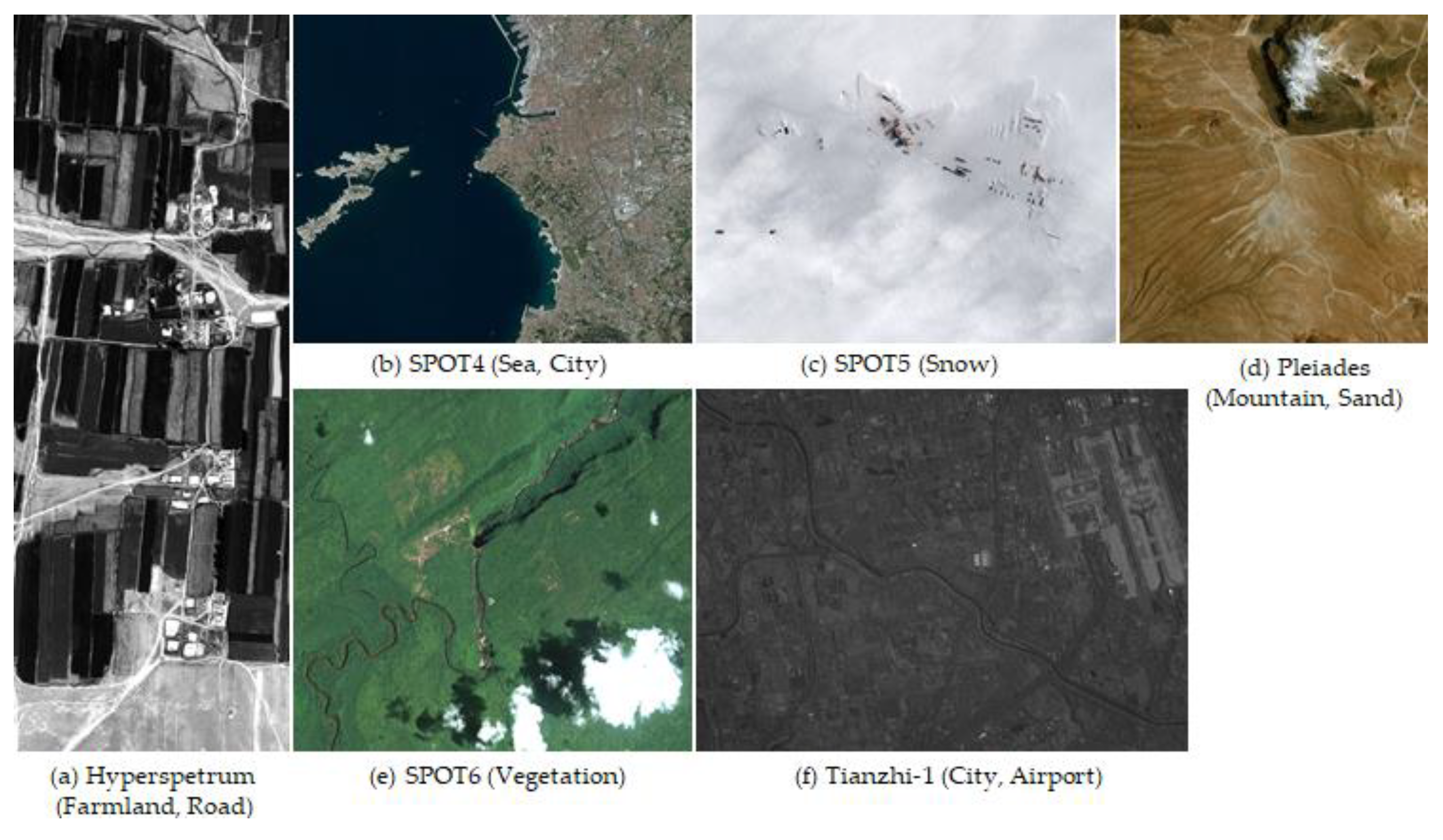
2.1. The Dataset

After a satellite is put into orbit, the SNR performance of the remote sensing payloads can only be estimated on remote sensing images. In this study, the experimental data in

Table 1. The basic information of plain images.

Satellite	Sensor	Size (Pixel)	Frame	GSD (m)
Tianzhi-1	pan	2048 × 2560	10	6
SPOT4	pan/multi	2048 × 2000	10	10/20
SPOT5	pan/multi	2000 × 2000	6	2.5/10
SPOT6	pan/multi	2500 × 2500	6	1.5/6
Pleiades	multi	3200 × 2500	8	2
UAV	hyper	2750 × 1030	1	2

are all remote sensing imagery. The noisy image dataset is obtained by the superposition of the original signal and the white Gaussian noise. Thus, the noise variance levels are known. However, the texture information in an image increases the evaluation errors. After reducing texture information, white Gaussian noise could be learned by neural networks. Answering the question of how to reduce the interference of ground objects is the key to manufacturing the dataset.

The imaging process of the ground objects captured by an remote sensor on its focal plane can be described as below:

Image = A × (Landscape ⊗ PSF) (x,y) × ∑δ(x-j × △x, y-i × △y) + noise,

(1)

Landscape is the ground objects, which is a continuous function of spatial variables (x,y). Additionally, its value is directly proportional to the ground object irradiance entering a remote sensor. After convolution operation with the point spread function—PSF—Landscape is sampled by the focal plane CCDs with sampling intervals of △x and △y.

According to Equation (1), the approximately noise-free dataset at a specified ground sample resolution could be obtained after mean filtering and downsampling. Additionally, different levels of white Gaussian noise are added into the data to construct simulated data with known true-noise SDs. The data processing is summarized as follows: (1) 3 × 3 mean filtering on the original data; (2) two (or more) instances of downsampling to obtain images without noise; (3) the division of images into small blocks with 32 × 32 pixels; (4) the addition of white Gaussian noise to the data.

In the cases of differences in dynamic ranges or imaging conditions for different remote sensors, the same noise levels make some data appear saturated and degraded. Therefore, the principle of adding noise is: the noise added into images could not exceed the signal power. Considering the principle, the maximum noise variance added into images was σ² = 20.

The input of the model is a small block with a size of 32 × 32 pixels. Thus, images are also divided into 32 × 32 pixels. Additionally, each image is randomly divided, and the number is 50% of the formatted division. In addition, some small blocks are rotated and mirrored to increase the robustness of the model and the expansion of the dataset. The information is shown in

Table 2. The information of the dataset, generated from the plain images.

Original Data	Training Samples	Validating Samples	Testing Samples
Tianzhi-1	3840	2560	1280
SPOT4	2976	1984	992
SPOT5	2883	1922	961
SPOT6	4563	3042	1521
Pleiades	5850	3180	1950
UAV	20,112	12,688	6704

.

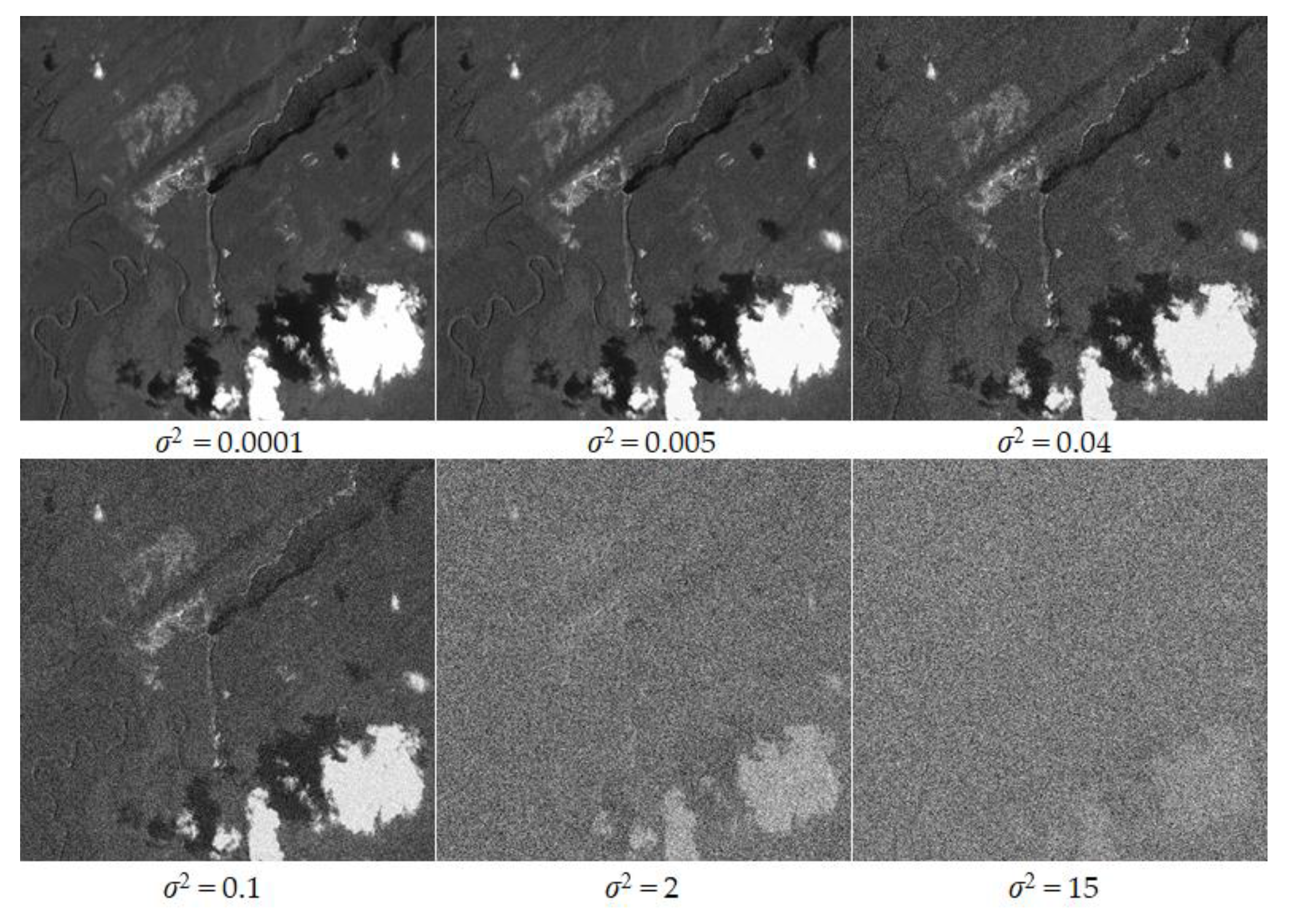
2.2. Experiment Introduction

In order to validate the effectiveness of the proposed method, several of the typically traditional methods on SNR estimation and a denoising method based on a convolutional neural network were selected to compare and analyze, including LSD [7], FFT-DC [12], ReSNR [13], SDC [11], Yu [20], and DnCNN [14]. A total of 6 unused images were selected as the experimental basic data (shown in Figure 1). Additionally, 6 different noise levels were added into each image. The noise variances were 0.0001, 0.005, 0.04, 0.1, 2 and 15, respectively. Additionally, the mean values of the noise were all 0. These methods were evaluated and compared on the accuracy of noise estimation.

3. The Proposed Method

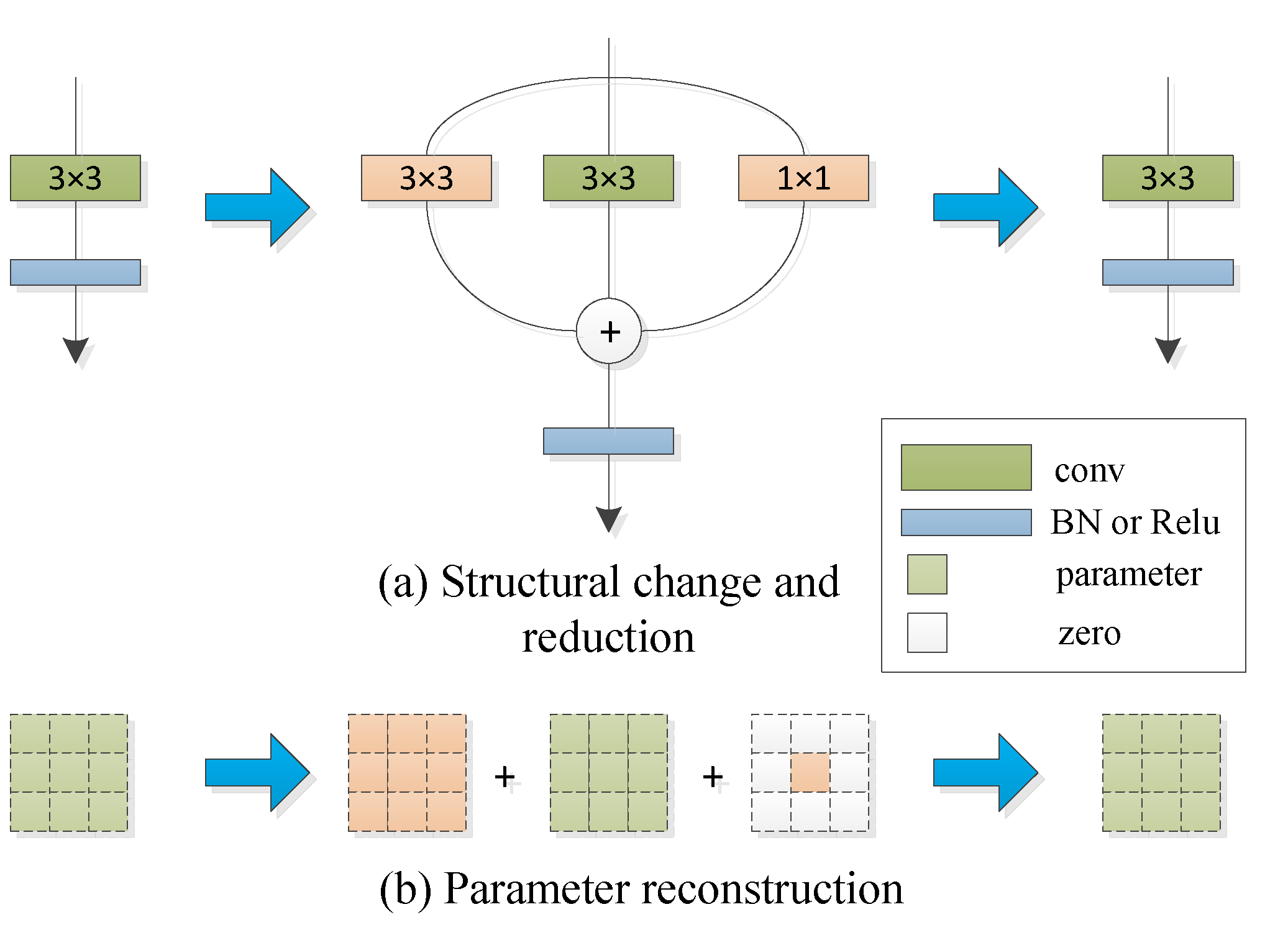
3.1. Multi-Branch Training and Parameter Reconstruction

Generally speaking (regardless of gradient vanishing or explosion), the deeper or wider a neural network is the more feature information it learns. In other words, under the same depth, wider networks learn more target features, such as GoogLeNet [22]; under the same width, deeper networks also improve the feature analysis, such as VGG16 [23] and ResNet [24]. Compared with VGG, multi-branch networks often have better regression and classification effects. However, the structure of the chain-convolutional neural network similar to VGG is simple and compact, and chain networks are easier to be distributed. Comprehensively considering the advantages of the multi-branch structure and the lightweight goal, the novel method of multi-branch training and parameter reconstruction inference was designed to improve the application efficiency of lightweight neural networks, similar to VGG. The novelty is summarized as follows: (1) Multi-branch training learns more feature information and reduces over-fitting due to enhanced feature maps. (2) Parameter reconstruction preserves the original structure after training. (3) It achieves the inference effects of a multi-branch network, compared with the original network. The total weight parameters do not increase while inferring, although the local structure becomes wider when training.

Figure 2a shows the structural changes when training. One group of convolutions is appended with several different groups such as two extra groups of convolutions with 3 × 3 and 1 × 1 size, respectively. It makes the network learn more feature information than the original group. Figure 2b shows the process of parameter reconstruction, which remains as the structure of the original network after training. The new process of converting several trained groups into one group of convolution layers for inference is described as follows.

Assuming W_i∈ℝ^C1×C2×3×3 to denote the 3 × 3 convolution layer with C₁ inputs and C₂ output channels, b_i∈ℝ^C1×C2 denotes the offsets. Then, the output feature map Y_i is:

Y_i = W_i ⊗ X + b_i,

(2)

Y = ∑Y_i = ∑(W_i ⊗ X + b_i) = ∑(W_i) ⊗ X + ∑(b_i) = W ⊗ X + b,

(3)

where ⊗ is the convolution operator. Y is the output of the structure of parallel convolutions. W is the integrated weight parameters. b is the integrated offset. The description of the gradient backward propagation is:

$$\frac{dY}{dX}={{\displaystyle \sum }}^{ }\frac{\partial Y_i}{\partial X}={{\displaystyle \sum }}^{ }\frac{\partial \left(W_{i}X+b_i\right)}{\partial X}={{\displaystyle \sum }}^{ }\frac{\partial \left(W_{i}X\right)}{\partial X}+{{\displaystyle \sum }}^{ }\frac{\partial b_i}{\partial X}={{\displaystyle \sum }}^{ }{W}_i$$

(4)

Note that the number, size, and moving strip of convolution kernels must be the same. For lightweight networks, a kernel of a 3 × 3 size is recommended. Small convolution kernels could achieve the effects of large size convolution kernels, and the amount of parameters is lower than a larger convolution kernel. For example, a 5 × 5 size convolution operation is equivalent to two 3 × 3 size convolution operations. In addition, small kernels expand perceiving areas [25].

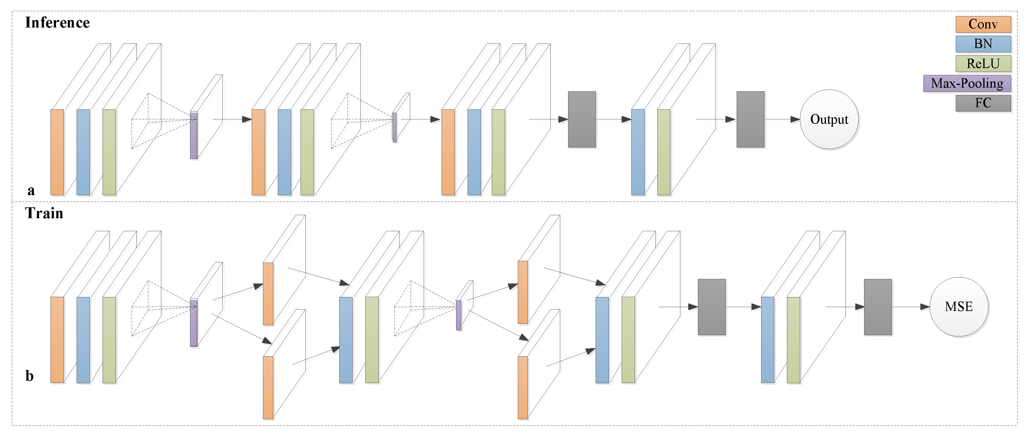
3.2. SNR Neural Network

Figure 3 shows the proposed CNN structure. The inference network (Figure 3a) has five main weight layers including three convolution layers (conv) and two full connection layers (FC). In addition, it contains four batch normalization [26] layers (BN). The activation functions are all ReLU [27]. The pooling method is the maximum pooling [28]. Adam [29] is chosen as the gradient updating method. Finally, the output of the model is the standard deviation of the noise.

The main training process is almost the same as the inference. The difference is in the second and third convolution process: two parallel convolutions are used instead of one single convolution (Figure 3b). The output feature maps of two parallel convolutions are performed “plus” an operation at the corresponding channels and pixel positions. After that, the size of the integrated feature map is the same as that of the feature map generated by one single convolution, as is the number of channels. The neural network realizes the regressively fitting task, not the classification task, thus the mean square error (MSE) is selected as the loss function. The main weight parameters of the training and inference networks are shown in

Table 3. The weight parameters of training and inference.

Params	Size	Strip	Count	Training	Inference
Conv 1	3 × 3	1	16	√	√
BN	16 × 32 × 32	--	--	√	√
Conv 2	3 × 3	1	32	√	Conv 2,Conv 3integrated
Conv 3	3 × 3	1	32	√
BN	32 × 16 × 16	--	--	√	√
Conv 4	3 × 3	1	64	√	Conv 4,Conv 5integrated
Conv 5	3 × 3	1	64	√
BN	64 × 8 × 8	--	--	√	√
FC 1	64 × 8 × 8 × 2	--	--	√	√
BN	2	--	--	√	√
FC 2	2 × 1	--	--	√	√
Activation Function: ReLU			Params Updating: Adam
Initialized Weight: He			Learning Rate: 0.0001
Input Size: 32 × 32			Output: Noise SD

.

4. Results and Analysis

4.1. Comparison of Training Results Based on Neural Network

Our model and the model in [20] are both neural networks that are similar to VGG. Both of them evaluate SNR directly rather than denoise. Therefore, the two models are compared and analyzed. Firstly, both of the two are trained in traditional methods. Following this, they were trained in the novel method: (1) the model in [20] was trained in the traditional training method, denoted as Net-1; (2) Net-1-M was the model of Net-1 that was trained in the novel method; (3) our model was trained in the traditional method, denoted as Net-2; and (4) Net-2-M was the model of Net-2 that was trained in the novel method.

The root mean square error (RMSE) measures the deviations between the estimated and the true values, which is described as follows:

$$RMSE=\sqrt[2]{\frac{1}{N}{{\displaystyle \sum }}_{k=1}^N{\left(\sigma -{\sigma }_0\right)}^2}$$

(5)

where σ₀ is the true noise SD, σ is the estimated SD, and N is the number of σ. The training results are shown in Figure 4.

Figure 4 shows the training results for the four cases described above. The deviation estimated by Net-1-M (yellow), trained in the multi-branch method, is closer to true value and less than that of Net-1 (blue), trained in the traditional method. Meanwhile, the deviation estimated by Net-2 (green), trained in the traditional method, is also significantly higher than that of Net-2-M (red), trained in the multi-branch method. The comparative experiments show that the multi-branch training could improve the ability of the CNNs that are similar to VGG, and its training effect is higher than that of the traditional training method.

The parallel multiple convolutions extract different feature maps. Additionally, they are integrated into one feature map. On one hand, integration makes the feature information rich and avoids overfitting to some extent. On the other hand, the upstream gradient is passed to each branch when the gradient is propagated backward. Additionally, the gradient attenuation of each branch is the same, which accelerates the gradient updating and makes the whole of the training process converge fast. After going through many forward and backward propagations, each branch learns different features that tend to express the abstract features of targets. However, CNNs that are similar to VGG and trained in the traditional method need more epoch time or a deeper structure to achieve a better performance. The yellow (Net-1-M) and green (Net-2) curves in Figure 4 illustrate the situation: the results estimated by Net-1-M were close to those of Net-2, which had a deeper network. Net-2 had one FC layer, one BN layer, and one more ReLU layer than Net-1-M. Our model trained in the multi-branch method (Net-2-M) achieved better training effects—the smallest RMSE and a faster convergence (red curve in Figure 4).

4.2. Accuracy Validation with Known Noise Levels

For validating the accuracy of our model, the methods described in Section 2.2 were selected for contrast and analysis. Additionally, the different noise levels described in Section 2.2 were added into Figure 1. Take Figure 1e as an example of a noisy image (shown in Figure 5).

The image degrades seriously when the noise variances are 2 and 15, which conflicts with the principles described in Section 2. However, they are still retained to validate the performances of these methods. Different noises are added into each image to manufacture noisy images. In order to facilitate a statistical analysis and display, the estimated noise SDs in the same noise levels are summed, and their mean values are computed. The results are shown in

Table 4. The noise estimation results of the references and the proposed model.

Method	Noise Standard Deviation
	0.01	0.07	0.2	0.316	1.41	3.87
LSD	2.96	18.7	45.9	63	75.6	63.7
FFT-DC	2.77	5.66	2.41	1.76	1.04	1.17
ReSNR	5.43	5.28	2.23	1.61	0.86	1.01
DnCNN 1	6.98	17.9	18.7	19.2	24.3	26.8
Net-1 1	0.033	0.027	0.123	0.233	1.6	2.67
Net-2-M 1	0.036	0.063	0.187	0.282	1.4	2.67
Method	Root Mean Square Error (RMSE)
LSD	2.99	18.7	45.9	62.9	74.3	67.4
FFT-DC	2.78	6.39	2.53	1.66	0.61	2.7
ReSNR	5.7	6.0	2.35	1.49	0.4	2.86
DnCNN 1	7.11	17.8	18.5	18.9	22.91	22.88
Net-1 1	0.027	0.04	0.085	0.083	0.188	1.202
Net-2-M 1	0.03	0.014	0.03	0.04	0.08	1.197

¹ CNN models.

.

Table 4 shows the noise estimated by the traditional and neural-network-based algorithms. These methods are tested on noisy images, of which the noise levels are known clearly. The neural-network-based methods obtain less deviation errors than the traditional ones, which are mainly affected by different texture features and uneven distributions of ground surfaces. The proposed CNN trained in the novel method achieves an average RMSE of 3.9%. Meanwhile, the Net-1 trained in the traditional method achieves 8.5%. Other methods achieve larger errors. These statistics do not include the last group of data. This is because the last group of data is gathered from the images of which the noise intensity is higher than the signal. In general, the neural-network-based methods perform better than the traditional methods for different noise levels. Additionally, the proposed method is more accurate than other reference methods.

Figure 6 shows that the accuracy of the traditional methods on the images with uniform land surfaces (Figure 1e,f) is higher than the complicated land surfaces. Thus, the traditional methods are applied on images with many uniform or homogeneous areas. For the denoising method DnCNN, the performance is general. The aim of denoising is to improve quality by refining details, enhancing contrast, etc. The residual noise contains part of the image information, which causes high noise estimation. Figure 7 shows the difference between the noise obtained by DnCNN and the true noise distribution. The red box in Figure 7a shows that the texture structure is left in the noisy image when compared with the true noise (shown in Figure 7b), which causes a large estimated variance of 0.04, while the true noise variance is 0.005. The methods based on convolutional neural network try to find the mapping relationship between the noise and the noisy signals. In the mapping relationship, several groups of weight parameters are trained to maximize the satisfaction of the results that conform to the true situation. The noise levels achieved by CNNs are closer to the true noise levels. Figure 8 shows the situation and displays the changing rates between the estimated and the true values.

To further analyze Figure 8a–c, most of the estimated values are in the upper left, but the noise SDs are not high (<0.5). This is because the traditional methods (a–c) are greatly affected by the uneven ground surfaces. With the noise level increasing up, the estimated values become larger or smaller (black circles gathered at the top right or bottom right), which indicates these methods are affected seriously by noise intensity. Additionally, most of these methods show large errors for the seriously degraded images. For Figure 8d–f, the R values are 0.7205, 0.9733, and 0.98546, respectively. They are closer to 1.0. Meanwhile, our model achieves the best performance: R is 0.98546 in Figure 8f.

With respect to Figure 4 and Figure 8 and Table 4, the traditional and CNN-based algorithms comparisons can be drawn, validating our proposed approach: accuracy is increased when training a CNN similar to VGG in a novel method.

4.3. SNR Estimation on Blind Imagery

The experiment was considered from two aspects: (1) a comparison between estimated SNRs and calibrated SNRs in a laboratory, and (2) a spectral response curve trend, in particular, several spectral bands with strong absorption and reflection. Blind images were real remote sensing images without noise filtering and downsampling, etc. The SDC dedicated to estimating hyperspectral SNRs and the Net-1 method were selected as the reference methods. An L1A level [30] hyperspectral with 128 bands was selected as the test data, which is shown in Figure 1a. The SNRs of the hyperspectral sensor were calibrated before the aerial photography. Most of the hyperspectral bands had SNRs greater than 30 dB, and the average SNR was 40 dB. The SNR equation is described as follows:

$$SNR=\frac{E}{\sigma }$$

(6)

$$SN{R}_{dB}=20{\log }_{10}SNR,$$

(7)

where E is the mean gray value of single band image, σ is the noise standard deviation, and SNR_dB is the decibel intensity of SNR.

Figure 9 shows the estimated SNR results. The different colors correspond to the three different methods: SDC (blue), Net-1 (orange), and Net-2-M (red). The average SNRs evaluated by the three methods are 29.8 dB, 34.5 dB, and 37.8 dB, respectively. Combined with the calibrated SNRs, with a total average of 40 dB, the average accuracy of Net-1 and Net-2-M are better than the SDC in Figure 9a, of which Net-2-M performs best (5.5% relative error on average). Combined with the analysis of the average gray level of each spectral band (shown in Figure 9b), the gray values of the first ten and the last ten bands are relatively smaller than others. Then, the SNRs should show an upward trend at the beginning and a downward trend at the end. In this case, all of the three methods show the same trend. Due to the unique spectrum absorption of chlorophyll in green vegetation near the 450 nm and 650 nm [31] (band 4 and 12 in Figure 9) wavelengths, the signals are weaker than the adjacent bands, which causes the SNRs to be smaller than the adjacent bands. Corresponding to this case, SDC and Net-2-M display similar trends, but Net-1 shows the difference. In addition, there is a “red edge” effect near 700 nm–950 nm (band 16–36) [32], and the signal strengths increase up sharply. Thus, the SNRs show an upward trend. Both SDC and Net-2-M follow these characteristics on the SNR curve. Meanwhile, the Net-1 curve is relatively flat and gentle. Since the water in plant tissues absorbs sunlight at the wavelengths of 1450 nm and 1190 nm [33] (band 76 and 112), the signals are also weak. Both of the SDC and Net-2-M curves show the situation. In summary, the SNR curve obtained by Net-2-M is consistent with the trend in the specific spectral response curve.

The three methods are compared and analyzed in terms of the average accuracy and SNR trends at the specific spectrum response bands: (1) Net-2-M performs the best in accuracy (37.5 dB closest to the calibrated 40 dB on average); (2) Net-1 performs well on overall trends, but its local accuracy is insufficient. It is necessary to either increase the training epochs or deepen the neural network such as in Net-2; and (3) SDC is stable, but the average accuracy is lower than the other two methods.

5. Discussion

In this study, we contributed two important aspects: (1) The design of a lightweight CNN for SNR estimation; (2) The proposal of a novel training and parameter-reconstructed inference method to enhance traditional CNNs that are similar to VGG. The experimental results prove the effectiveness of our work.

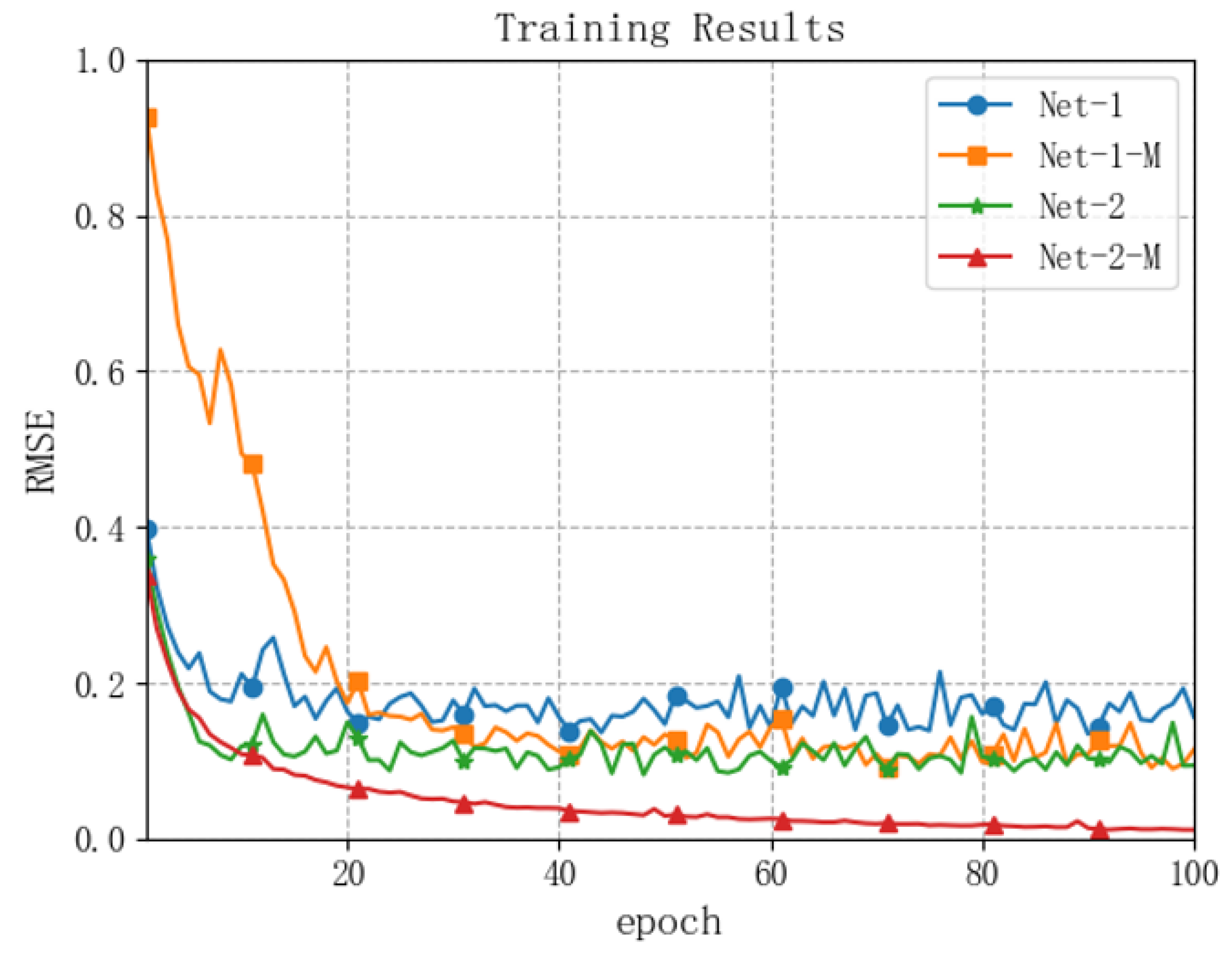
• In this study, [20] and the proposed models (Net-1 and Net-2 in Figure 4) are compared. The two CNNs are trained in the traditional method. Net-2 has one more FC layer and one more BN layer than Net-1. When comparing the results of the two CNNs on the dataset, the deeper network (Net-2) performs better. Regardless of the gradient vanishing, the appropriate deepening of a neural network would extract more abstract and useful feature information [34,35]. The useful information transmitting could reduce the redundant and interfering information to a certain degree.
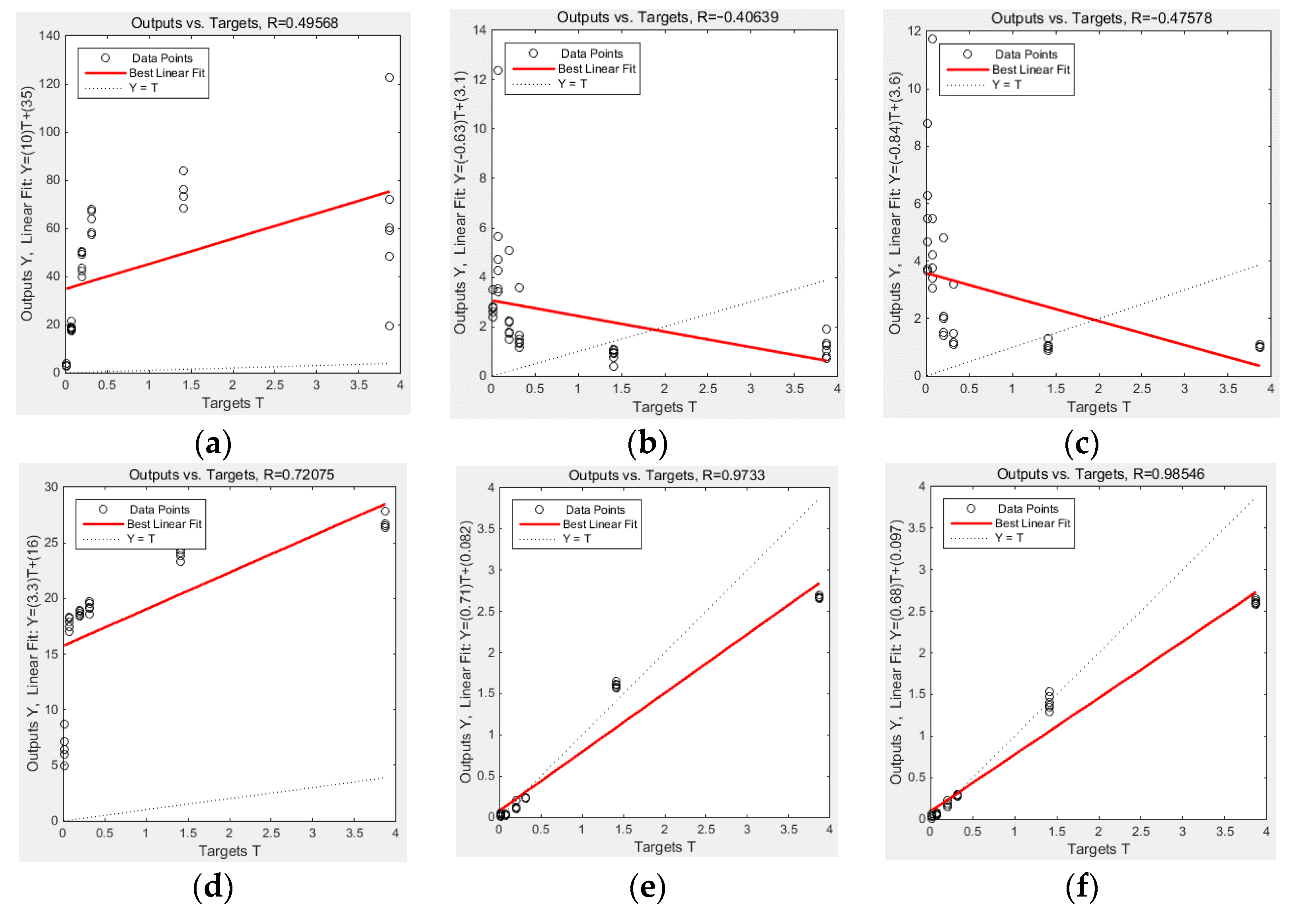
• In the comparative experiment, there is another analyzable test: a comparison between traditional training and multi-branch training. Figure 4 shows that the multi-branch training method is more accurate than the traditional training method. The reasons are: (a) multiple branches extract more useful features than one branch and achieve the effect of a deeper network; and (b) during the backward propagation, the upstream gradients are passed to each branch, and the gradient attenuation of each branch is the same. It accelerates the gradient updating and makes the whole training process converge quickly, which reduces the training time. For example, the training epochs of Net-1-M are less than Net-1, but the average RMSE obtained by Net-1-M is minimal; the RMSE obtained by Net-1-M is close to Net-2, but Net-1-M has less layers than Net-2.
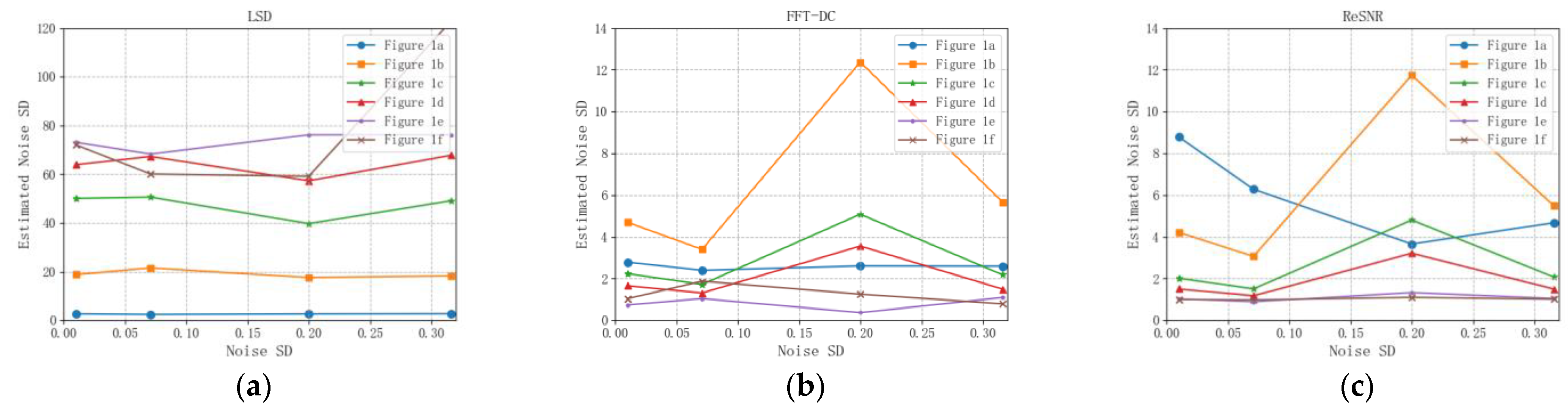
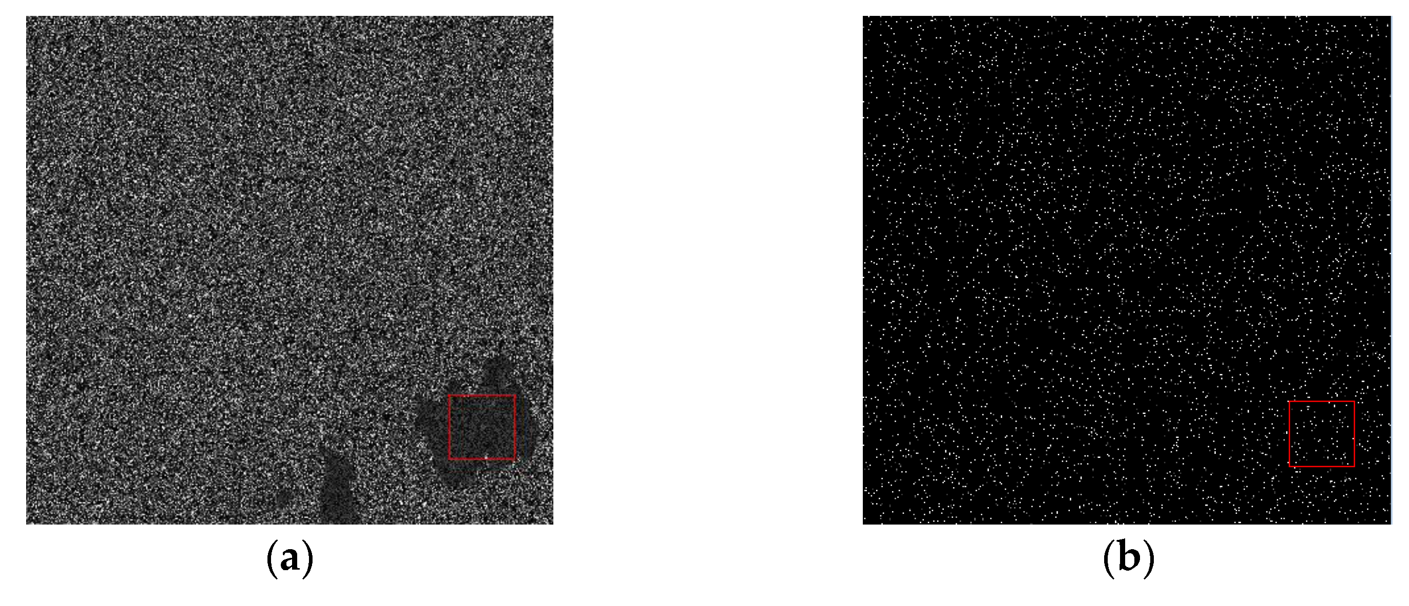
• For the accuracy tested on the noise-known images, five methods are used as reference methods. The dataset contains different scenes such as farmland, roads, city, sea, mountain and vegetation, etc. When compared with each method, the proposed method is still better than others. The traditional methods are limited by heterogeneous or complicated land surfaces [9,12]. For the denoising DnCNN, the residual noise tends to contain part of the image structure information, which causes the high error of noise estimation (shown in Figure 7). Unlike denoising DnCNN, our model learned the feature of Gaussian noise rather than the ground features. For different land surfaces, our model still performed well.
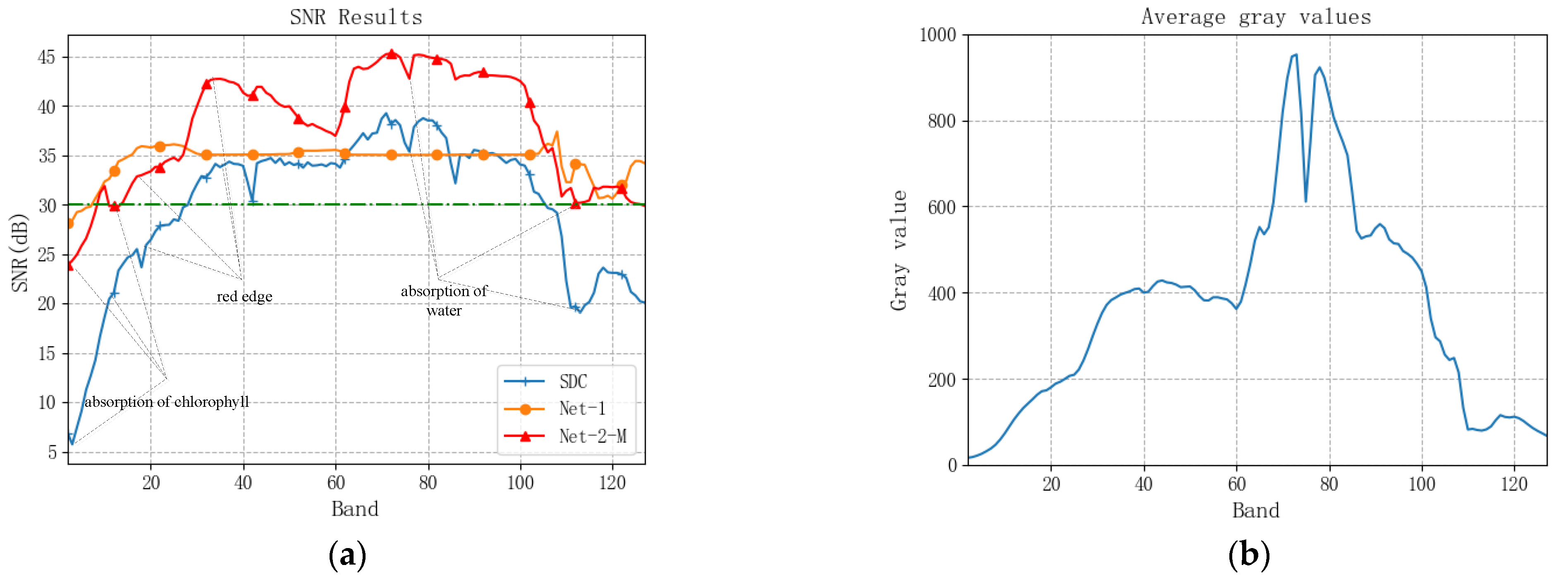
• In the test on blind imagery, three methods (SDC, Net-1, and Net-2-M) are used to estimate SNR on real hyperspectral imagery with 128 bands captured by a UAV flight. The SNRs of the remote sensor are calibrated in the laboratory before aerial photography: 40 dB on average for 128 bands. Compared with the calibrated SNRs, the Net-1 and Net-2-M are more accurate than SDC, which is restricted to the complicated ground features. For optical remote sensors, thermal noise hardly changes with signals [36] under stable conditions. In other words, thermal noise is affected by temperature changing and hardly affected by spectrum frequency. Then, at the absorption or reflection bands, the SNRs are lower or higher than those adjacent bands. In this case, the SNR curve obtained by Net-2-M is consistent with the specific spectral response compared with the other two methods.
• The performance is not ideal for the proposed method in this case as the noise intensity increases, and the RMSE also increases (shown in Table 4). The reasons for this are: (a) the noise intensity is close to the signal, which causes serious image degradation. Thus, it is hard to distinguish signal and noise; and (b) the cases that do not meet the mapping relationship are not effectively excluded in the inference process. However, the traditional methods consider the cases by eliminating non-homogeneous information. To solve the problems, we can consider two aspects in the follow-up research: (a) analyze the uniformity of the input image block before inference; and (b) eliminate the image blocks in which data exceeds the mapping relationship.

6. Conclusions

In the context of estimating the SNRs of remote sensors on orbit and, more specifically, making an estimation based on CNN, we proposed a lightweight CNN and a novel training method of multi-branch training and parameter-reconstructed inference. The proposed CNN and the novel method are evaluated with other reference methods on three experiments such as the comparison of training results based on neural networks, accuracy validation with known noise levels, and SNR estimations on blind imagery. The first experiment proves that CNNs that are similar to VGG and trained by the novel method are faster at convergence and show a smaller RMSE than the traditional training methods. The second experiment demonstrates that the proposed CNN performs the best in the accuracy test and is less affected by texture features than the reference methods. The third experiment also proves the accuracy from another side. The results show that the proposed model has provided an increase in the evaluation performance when estimated with average accuracy and spectrum characteristics. In the future, the proposed model needs to be improved in ways such as combining the advantages of traditional algorithms and considering multiplicative noise. More tests need to be performed to validate the effectiveness of the proposed CNN and the novel training method.

References

- Shao, L.; Yan, R.; Li, X.; Liu, Y. From heuristic optimization to dictionary learning: A review and comprehensive comparison of image denoising algorithms. IEEE Trans. Cybern. 2013, 44, 1001–1013. [Google Scholar] [CrossRef]
- Xu, X.J.; Tang, L.; Kuang, N.L.; Liu, Y.Y. An image noise reduction and haze removal algorithm based on multi-frame merge. Microelectron. Comput. 2021, 9, 21708–21720. [Google Scholar]
- Khmag, A.; Ramli, A.R.; AI-Haddad, S.A.R.; Kamarudin, N. Natural image noise level estimation based on local statistics for blind noise reduction. Vis. Comput. 2018, 34, 575–587. [Google Scholar] [CrossRef]
- Curran, P.J.; Dungan, J.L. Estimation of signal-to-noise: A new procedure applied to AVIRIS data. IEEE Trans. Geosci. Remote Sens. 1989, 27, 620–628. [Google Scholar] [CrossRef]
- Eklundh, L.R. Noise Estimation in NOAA AVHRR Maximum-value Composite NDVI Images. Int. J. Remote Sens. 1995, 16, 2955–2962. [Google Scholar] [CrossRef]
- Chen, G.Y.; Zhu, F.Y.; Heng, P.A. An Efficient Statistical Method for Image Noise Level Estimation. In Proceedings of the 2015 IEEE International Conference on Computer Vision (ICCV), Santiago, Chile, 13–16 December 2015. [Google Scholar]
- Gao, B.C. An Operational method for Estimating Signal to Noise Ratios from Data Acquired with Imaging Spectrometers. Remote Sens. Environ. 1993, 43, 23–33. [Google Scholar] [CrossRef]
- Gao, L.R.; Zhang, B.; Zhang, X.; Shen, Q. Study on the Method for Estimating the Noise in Remote Sensing Images Based on Local Standard Deviations. Int. J. Remote Sens. 2007, 11, 203–208. [Google Scholar]
- Zhu, B.; Wang, X.H.; Tang, L.L.; Li, C.R. Review on Methods for SNR Estimation of Optical Remote Sensing Imagery. Remote Sens. Technol. Appl. 2010, 25, 303–309. [Google Scholar]
- Fu, P.; Sun, Q.S.; Ji, Z.X. Noise Estimation from Remote Sensing Images by Fractal Theory and Adaptive Image Block Division. Acta Geod. Cartogr. Sin. 2015, 44, 1235–1245. [Google Scholar]
- Roger, R.E.; Arnold, J.F. Reliably Estimating the Noise in AVIRIS Hyper Spectral Images. Int. J. Remote Sens. 1996, 17, 1951–1962. [Google Scholar] [CrossRef]
- Zhu, B.; Wang, X.H.; Li, Z.Y.; Dou, S.; Tang, L.L.; Li, C.R. A New Method based on Spatial Dimension Correlation and Fast Fourier Transform for SNR Estimation in Remote Sensing Images. In Proceedings of the 2013 IEEE International Geoscience and Remote Sensing Symposium (IGARSS 2013), Melbourne, Australia, 21–26 July 2013. [Google Scholar]
- Zhu, B.; Li, C.R.; Wang, X.H.; Wang, C.L. A New Method to Estimate SNR of Remote Sensing Imagery. In Proceedings of the 2017 SPIE: Optical Sensing and Imaging Technology and Applications, Beijing, China, 4–6 June 2017. [Google Scholar]
- Zhang, K.; Zuo, W.M.; Chen, Y.J.; Meng, D.Y.; Zhang, L. Beyond a Gaussian Denoiser: Residual Learning of Deep CNN for Image Denoising. IEEE Trans. Image Process. 2017, 26, 3142–3155. [Google Scholar] [CrossRef] [Green Version]
- Chen, Y.; Pock, T. Trainable nonlinear reaction diffusion: A flexible framework for fast and effective image restoration. IEEE Trans. Pattern Anal. Mach. Intell. 2017, 39, 1256–1272. [Google Scholar] [CrossRef] [Green Version]
- Yang, G.L. Research on Image Denoising Method Based on Convolutional Neural Network. Master’s Thesis, Nanchang University, Nanchang, China, 9 June 2020. [Google Scholar]
- Qin, Y.; Zhao, E.G. An Image Multi-Type Noise Removal Algorithm based on Lightweight Deep Residual Network. Comput. Appl. Softw. 2021, 38, 250–255. [Google Scholar]
- Delvit, J.M.; Leger, D.; Roques, S.; Valorge, C.; Viallefont-Robinet, F. Signal to Noise Assessment from Non Specific Views. In Proceedings of the Image and Signal Processing for Remote Sensing VII, Toulouse, France, 17–22 September 2001. [Google Scholar]
- Li, H.Z.; Tian, Y.; Han, C.Y.; Wu, G.D.; Ma, D.M. Assessment of signal-to-noise ratio of space optical remote sensor using artificial neural network. Opto-Electron. Eng. 2006, 33, 44–49. [Google Scholar]
- Yu, H.W.; Yi, X.W.; Xu, S.P.; Liu, T.Y.; Li, C.X. A fast noise level estimation algorithm based on convolution neural network. J. Nanchang Univ. 2019, 43, 497–503. [Google Scholar]
- Cui, G.M. Research on Image Quality Improvement and Assessment for Optical Remote Sensing Image. Ph.D. Thesis, Zhejiang University, Zhejiang, China, 16 June 2016. [Google Scholar]
- Sergey, I.; Christian, S. Batch Normalization: Accelerating Deep Network Training by Reducing Internal Covariate Shift. arXiv 2015, arXiv:1502.03167. [Google Scholar]
- Nair, V.; Hinton, G.E. Rectified linear units improve restricted Boltzmann machine. In Proceedings of the 27th International Conference on Machine Learning (ICML-10), Haifa, Israel, 21–25 June 2010. [Google Scholar]
- Huang, G.; Liu, Z.; Weinberger, K.Q.; Maaten, L.V.D. Densely Connected Convolutional Networks. arXiv 2018, arXiv:1608.06993v5. [Google Scholar]
- Kingma, D.P.; Ba, J.L. ADAM: A method for stochastic optimization. International Conference on Learning Representations (ICLR). arXiv 2017, arXiv:1412.6980v9. [Google Scholar]
- Szegedy, C.; Liu, W.; Jia, Y.Q.; Sermanet, P.; Reed, S.; Anguelov, D.; Erhan, D.; Vanhoucke, V.; Rabinovich, A. Going deeper with convolutions. arXiv 2014, arXiv:1409.4842v1. [Google Scholar]
- Simonyan, K.; Zisserman, A. Very Deep Convolutional Networks for Large Scale Visual Recognition. arXiv 2015, arXiv:1409.1556v6. [Google Scholar]
- He, K.M.; Zhang, X.Y.; Ren, S.Q.; Sun, J. Deep Residual Learning for Image Recognition. arXiv 2016, arXiv:1512.03385v1. [Google Scholar]
- Saito, K.Y. Deep Learning from Scratch, 1st ed.; O’ Reilly Japan: Tokyo, Japan, 2016; pp. 240–242. ISBN 978-7-115-48558-8. [Google Scholar]
- Pre-Processing Product Levels for Spaceborne Hyperspectral Imaging Data; GB/T36301-2018. Standardization Administration of the People’s Republic of China: Beijing, China, 2019.
- Song, K.S.; Zhang, B.; Wang, Z.M.; Liu, H.J.; Duan, H.T. Inverse model for estimating soybean chlorophyll concentration using in-situ collected canopy hyperspectral data. Trans. CSAE 2006, 22, 16–21. [Google Scholar]
- Moran, J.N.; Mitchell, A.K.; Goodmanson, G.; Stockburger, K.A. Differentiation among effects of nitrogen fertilization treatments on conifer seedlings by foliar reflectance: A comparison of methods. Tree Physiol. 2000, 20, 1113–1120. [Google Scholar] [CrossRef] [Green Version]
- Qiao, X. The Primary Investigation in Diagnosing Nutrition Information of Crop Based on Hyperspectral Remote Sensing Technology. Master’s Thesis, Jilin University, Jilin, China, May 2005. [Google Scholar]
- Zeiler, M.D.; Fergus, R. Visualizing and Understanding Convolutional Networks. In Proceedings of the 13th European Conference on Computer Vision (ECCV), Zurich, Switzerland, 6–12 September 2014. [Google Scholar]
- Mahendran, A.; Vedaldi, A. Understanding deep image representations by inverting them. In Proceedings of the IEEE Conference on Computer Vision and Pattern Recognition (CVPR), Boston, MA, USA, 7–12 June 2015. [Google Scholar]
- Huang, S.J. Research on the Technology of Geosynchronous Orbit High Dynamic Range Information Acquisition. Ph.D. Thesis, University of Chinese Academy of Sciences, Beijing, China, May 2015. [Google Scholar]