Article

Rainfall Similarity Search Based on Deep Learning by Using Precipitation Images

College of Computer and Information, Hohai University, Nanjing 210098, China
*
Author to whom correspondence should be addressed.
Appl. Sci. 2023, 13(8), 4883; https://doi.org/10.3390/app13084883
Submission received: 22 February 2023 / Revised: 8 April 2023 / Accepted: 10 April 2023 / Published: 13 April 2023
(This article belongs to the Special Issue Deep Learning and Edge Computing for Internet of Things)

Abstract

:
Precipitation images play an important role in meteorological forecasting and flood forecasting, but how to characterize precipitation images and conduct rainfall similarity analysis is challenging and meaningful work. This paper proposes a rainfall similarity research method based on deep learning by using precipitation images. The algorithm first extracts regional precipitation, precipitation distribution, and precipitation center of the precipitation images and defines the similarity measures, respectively. Additionally, an ensemble weighting method of Normalized Discounted Cumulative Gain-Improved Particle Swarm Optimization (NDCG-IPSO) is proposed to weigh and fuse the three extracted features as the similarity measure of the precipitation image. During the experiment on similarity search for daily precipitation images in the Jialing River basin, the NDCG@10 of the search results reached 0.964, surpassing other methods. This indicates that the method proposed in this paper can better characterize the spatiotemporal characteristics of the precipitation image, thereby discovering similar rainfall processes and providing new ideas for hydrological forecasting.

1. Introduction

In recent years, flash floods caused by extreme rainfall have led to extensive social and economic losses [1]. Due to the influence of precipitation intensity, precipitation distribution, and other factors, there are many uncertainties in the time, location, grade, and process of floods, which pose great obstacles to early flood warning and prevention. Therefore, extracting spatiotemporal features of rainfall-runoff processes, identifying and classifying them, so as to discover similar rainfall-flood patterns from historical rainfall events to provide guidance and technical support for hydrological forecasting and water resource utilization, has become an urgent task in the application field of hydrology and water resources [2,3].
The rainfall-flood similarity analysis uses fuzzy mathematics, data mining, and machine learning methods to identify the similar (closest) sequence pairs to the current real-time rainfall-flood sequence from the historical hydrological time series patterns by defining the similarity measure [4]. The most direct application of rainfall-flood similarity analysis is to determine whether a current rainfall-flood process is similar or equivalent to a process in a historical period [5]. In this sense, research on similarity analysis methods has significant potential for rainfall-runoff process forecasting, environmental evolution analysis, and hydrological regularity discovery [6,7].
Rainfall similarity analysis is an important part of rainfall-flood similarity analysis and flood risk assessment [8]. It can not only discover the rules of similar rainfall-flood patterns in history but also provide new ideas and technical support for rainfall-flood forecasting. Zhang [9] established a similarity analysis model for precipitation stations using the K-means clustering algorithm based on the Davies–Bouldin index. Then the single precipitation type histogram similarity model was adapted to analyze the clustering results and obtain similar stations. Xiao [5] proposed a rainfall event similarity analysis model for rainfall forecasting, which evaluated the similarity between two rainfalls from multiple perspectives, such as the quantity similarity, pattern similarity, earth mover’s distance, and rainfall spatial distribution similarity; the experimental results showed the similar rainfall analysis method is effective and applicable. Ohno [10] developed a new forecasting technique for predicting whether water levels will exceed a ‘flood’ threshold or not by using deep learning methods based on weather forecast precipitation images, which provided a new idea and reference for extending the flood forecast period.
Traditional similarity analysis of rainfall mainly uses time series text data, which cannot effectively represent the spatial distribution of rainfall. Moreover, the existing research on rainfall similarity lacks comprehensive measurement methods for multivariate characteristics of rainfall and is greatly insufficient in terms of interpretation. In the past decade, with the development of information technology, the hydrological departments have accumulated a large amount of spatiotemporal data, and data types have been expanded from traditional time series to semi-structured and unstructured. As is shown in Figure 1, different colors represent different precipitation grade and provide the spatiotemporal distribution information of precipitation in the Jialing River Basin. However, as time and spatial scales accumulate, it becomes more difficult to discover useful knowledge from these increasingly big data. Therefore, utilizing the latest machine learning and artificial intelligence algorithms to carry out feature extraction and fast similarity analysis on the accumulated big data of precipitation images to provide technical support for the identification of similar rainfall-flood processes and flood control is becoming a meaningful and hot research issue [11,12].
This paper proposes a rainfall similarity research method based on deep learning by using precipitation images. The novelty of this article lies in that the regional precipitation, precipitation distribution, and precipitation center are extracted as the characters of the precipitation image, and then appropriate distance measures for each feature are defined to better characterize the similarity between images. After that, an ensemble weighting method of normalized depreciation cumulative gain-improved particle swarm optimization (NDCG-IPSO) is proposed to weight and fuse the distance measures of three extracted features as the similarity measure for daily precipitation image similarity search.
The remaining part of this paper is organized as follows: Section 2 presents the related work to this area of research. Section 3 presents the brief of NDCG-IPSO. Several experiments with the proposed method using real-world precipitation images are reported in Section 4. Finally, Section 5 gives conclusions and suggestions for further research.

2. Related Studies

2.1. Image Feature Extraction

Feature extraction (FE) is an important and necessary step in many processes related to image retrieval [13], image encryption [14], and pattern recognition [15], which was used to extract the most distinct and useful information presented in an image dataset, to form a low-dimensional feature space to represent and describe the images for the next searching, browsing, or retrieving. Generally, color, shape, and texture are common characteristics extracted for image retrieval [16].
As shown in Figure 1, the precipitation image has similar shape and texture features. Therefore, only the color features are extracted to characterize the different precipitation images. In this paper, the global color histogram is used to extract the color features of the precipitation image, and the regional precipitation of the basin is calculated according to the practical significance of each color. Moreover, the image is divided into m*n grids, and the block color histogram is used to extract more detailed information, such as spatial distribution and rainfall center, for a better description of the precipitation image.

2.2. Similarity Search

Similarity search (also known as the nearest neighbor search) is the problem of searching the data items that are nearest to a query item under some distance measure from a search (reference) dataset, which is the foundation for data mining tasks such as clustering and classification and has been applied to time series prediction in image retrieval. Generally, a similarity search relies on a distance measurement that quantifies how close two elements are in the feature space. The closer the elements are, the higher the similarity between them. Currently, there are many distance measurements, such as Minkowski distance [17], Dynamic Time Warping Distance (DTW) [18], and editing distance [19].
Minkowski distance is also known as Lp distance. If two time series Q = {q1, q2, …, qn} and C = {c1, c2, …, cn}, then the Minkowski distance D(Q, C) between Q and C is calculated as the following equation.
L p = D ( Q , C ) = ( i = 1 n | q i c i | p ) 1 p
The value of p is a positive integer. Minkowski distance is defined differently according to different values of p. If p = 1, L1 is called the Manhattan distance; if p = 2, L2 is called the Euclidean distance, which is the most widely used measure in time series similarity research; If p = ∞, L is the Chebyshev distance.

2.3. Deep Learning

Deep learning refers to a class of machine learning techniques which attempts to mimic the human brain, which is organized with a deep architecture and processes information through multiple stages of transformation and representation [20]. Deep learning methods allow a system to learn complex functions that directly map raw sensory input data to the output without relying on human-crafted features using domain knowledge [21]. Over the past several years, a rich family of deep learning techniques has been proposed and extensively applied to a variety of applications, including speech recognition, object recognition, and natural language processing, among others [22,23].
Particle Swarm Optimization (PSO) is a stochastic swarm-based deep learning optimization algorithm inspired by simulating a simplified social system of a flock of birds that fly towards their unknown destination (fitness function) in search of the locations of food resources [24]. The PSO algorithm is initialized with random particles (birds) with a specific position and velocity for the purpose of computing the objective function of an optimization problem. The best personal and global fitness positions are computed over each iteration of running the PSO algorithm. The position and velocity of each bird are updated according to the calculated fitness functions until the optimal solution is obtained. Assuming that in D-dimensional space, the location of the particle and the flight speed is expressed as the vector xi = [xi1, xi2, …, xiD] and vi= [vi1, vi2, …, viD], respectively. The position of the particle is updated as follows:
x i t + 1 = x i t + v i t + 1
The speed of the ith particle is updated as follows from iteration number to iteration number +1:
v i t + 1 = w v i t + c 1 r 1 ( p i b e s t t x i t ) + c 2 r 2 ( p g b e s t t x i t )
where w is the inertia weight, which represents the retention degree of the particle to the last velocity; c1 is the individual learning factor, which represents the learning ability of the particle to the individual optimal solution. c2 is the social learning factor, which represents the learning ability of the particle to the current optimal solution of the population. p i b e s t t is the individual optimal solution found by pi at time t; p g b e s t t is the population optimal solution found by the whole population particle at time t. In addition, the algorithm also has a parameter to represent the population size, that is, the number of particles, and a parameter to represent the maximum number of iterations of the algorithm.

3. Rainfall Similarity Search Based on NDCG-IPSO

The performance of the image search system crucially depends on the feature representation and similarity measurement. Therefore, the process of precipitation image similarity search mainly consists of two steps. Firstly, three features, namely the regional precipitation, the precipitation distribution, and the precipitation center, are extracted from the historical precipitation images and stored in the historical database. Then, the above three features are extracted from the precipitation image to be queried, and the images with higher similarity values are retrieved from the historical images as the similarity query results. The process flow of precipitation image matching is shown in Figure 2.

3.1. Feature Extraction

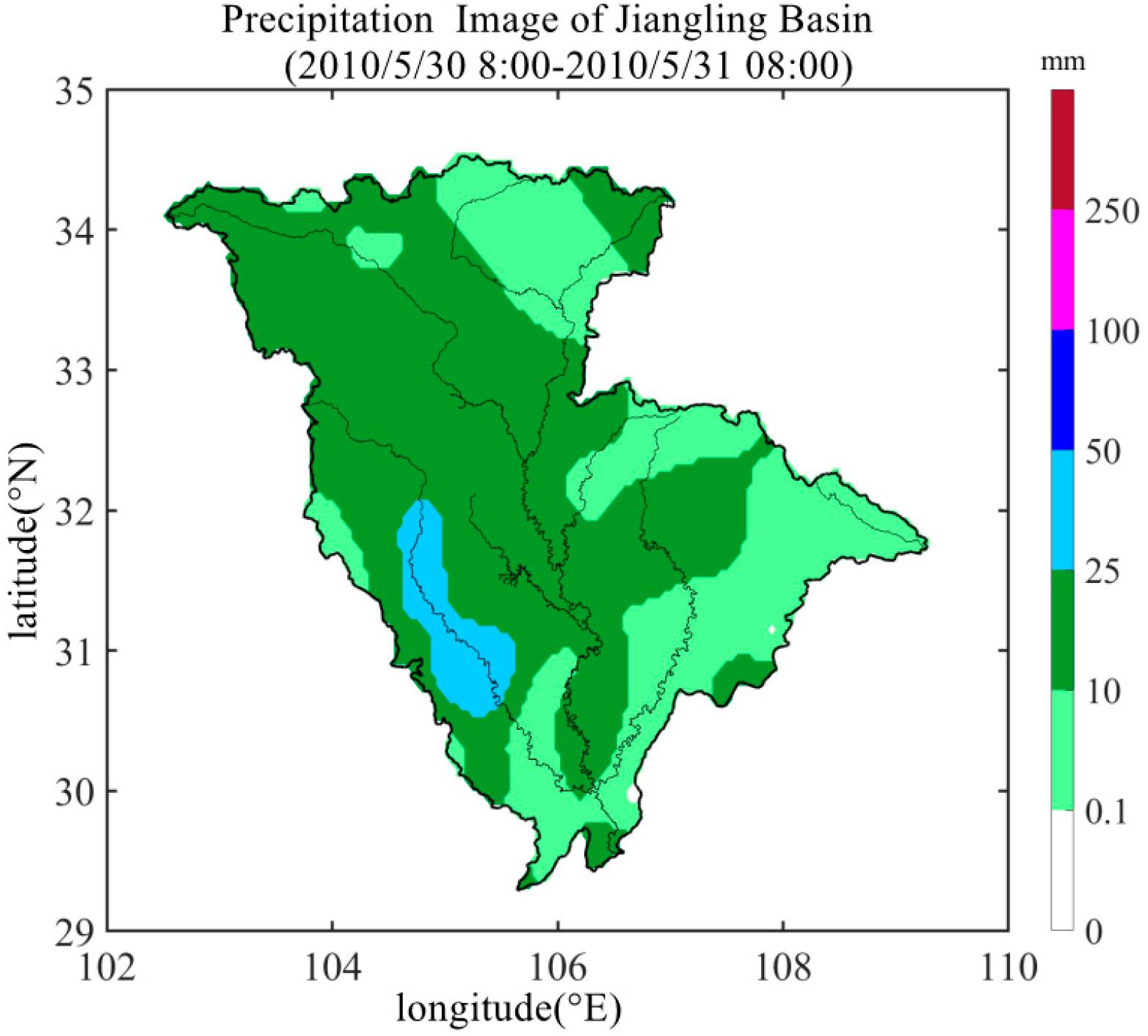
3.1.1. Regional Precipitation

Regional precipitation usually represents the total amount of precipitation within a given area at a specific time. In the precipitation image, each color corresponds to a range of precipitation amount. Hence, the regional precipitation feature can be obtained by weighting the color histogram, which can record the frequency of each color in the precipitation image.
Let the color histogram corresponding to the precipitation image contain K colors, namely C1, C2, …, CK, the occurrence number of each color in the image is num(Ci) (1 ≤ iK), and the precipitation amount corresponding to each color is pm(Ci), then the regional precipitation within a given area can be calculated as follows:
P = i = 1 K n u m ( C i ) p m ( C i )
Moreover, let P1 and P2 be the regional precipitation feature of the two precipitation images. The defined Manhattan distance Dp to measure the similarity between the regional precipitation features of the two images can be calculated as follows:
D P = | P 1 P 2 |

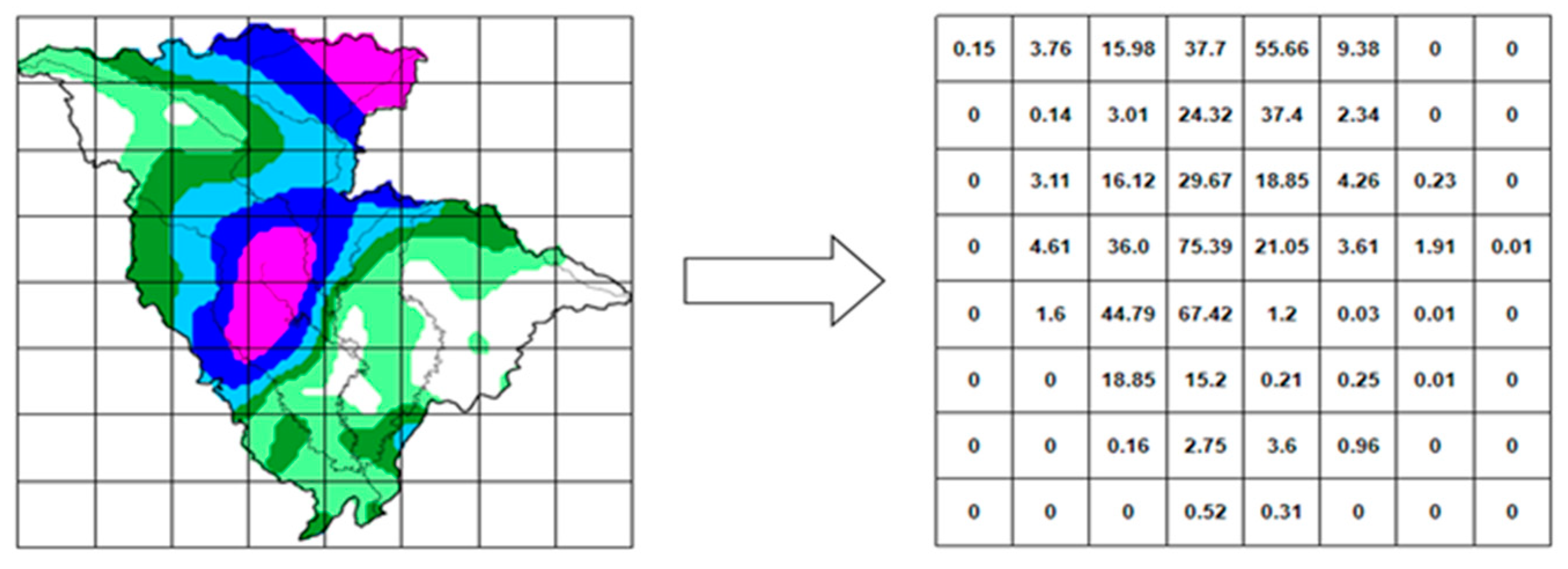
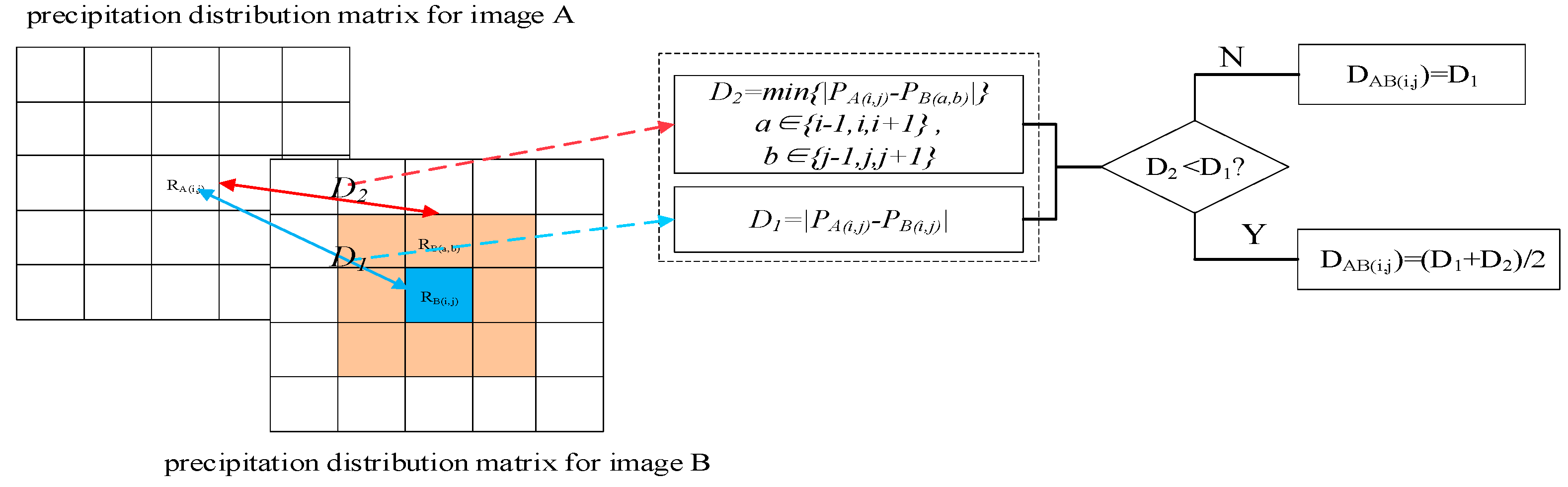
3.1.2. Precipitation Distribution

Regional precipitation can roughly represent the total amount of regional precipitation within a given area, but it is difficult to reflect the spatial distribution characteristics of precipitation. Therefore, the block-based color histogram is used to divide the watershed image into rectangular blocks with m rows and n columns after truncating redundant annotation. That is, the precipitation image is divided into m*n small grids. Additionally, the regional precipitation for each small grid can be calculated according to formula (4), respectively. Let P(i, j) be the regional precipitation for the grid located at the ith row and the jth column. The precipitation distribution matrix, denoted as R, is defined to characterize the spatial distribution feature for the precipitation image, which can be calculated as follows:
R = [ P ( 1 , 1 ) , P ( 1 , 2 ) , , P ( 1 , n ) P ( 2 , 1 ) , P ( 2 , 2 ) , , P ( 2 , n )                         P ( m , 1 ) , P ( m , 2 ) , , P ( m , n ) ]
Figure 3 shows the precipitation distribution matrix after blocking operation for the precipitation image.
Let R(a, b) be one of the blocks around R(i, j) in image B, where a ∈ {i − 1, i, i + 1}, b ∈ {j − 1, j, j + 1}. Let DAB(i, j) be the distance between elements in the ith row and the jth column of precipitation distribution matrix RA and RB, which can be calculated using the method shown in Figure 4. If the distance between RA(i, j) and RB(i, j), denoted as D1, is smaller than that between RA(i, j) and RB(a, b) (a ∈ {i − 1, i, i + 1}, b ∈ {j − 1, j, j + 1}), denoted as D2, DAB(i, j) can be represented by D1, else DAB(i, j) is represented by the mean of D1 and D2.
Thus, the distance of the precipitation distributions of two precipitation images, defined as DR, can be calculated as follows:
D R = i = 1 m j = 1 n D A B ( i , j )

3.1.3. Precipitation Center

Flood processes are largely influenced by the precipitation center. When the precipitation center is located upstream of the watershed, the long distance to the watershed section leads to a long lag time for the flood peak and presents a short and plump flood process. Meanwhile, when the precipitation center is located downstream, the short distance to the watershed section will make it a short lag time for the flood peak and form a sharp and thin flood hydrograph. Hence, it is important to take the precipitation center as a major feature in the precipitation image similarity research. Combined with the actual precipitation situation and image similarity retrieval requirements, take the block with the maximum precipitation in the precipitation image after being divided into blocks as the precipitation center.
Let P(i, j) be the maximum precipitation of the blocks in the precipitation image, then the precipitation center C(i, j) could be the block at the ith row and the jth column. Let C(i1, j1) and C(i2, j2) be the precipitation centers of two precipitation images. The Euclidean distance Dc is defined as the difference between the two precipitation centers, which can be calculated as follows:
D C = ( i 1 i 2 ) 2 + ( j 1 j 2 ) 2

3.2. Image Similarity Search Based on NDCG-IPSO

The precipitation image has different features. Hence, it may lose other feature information and reduce the accuracy of similarity retrieval if it applies a single feature to represent and measure the similarity of the precipitation image. Therefore, how to fuse the distances of the multiple features to represent the comprehensive distance between two precipitation images is becoming a necessary and urgent task. Given two precipitation images A and B, let DP, DR, and DC represent the regional precipitation distance, precipitation distribution distance, and precipitation center distance between two images, respectively, the fusion distance D between two images A and B can be calculated as follows:
D = γ 1 D P + γ 2 D R + γ 3 D C
where γ1, γ2, and γ3 are undetermined coefficient weights for the distance of regional precipitation, precipitation distribution, and precipitation center.
There are three kinds of methods namely the subjective weight method, objective weight method, and subjective-objective comprehensive weight method, to determine the undetermined coefficient. Subjective weighting relies on expert’s experiential knowledge, leading to subjectivity and variability. Objective weighting depends on the problem domain and sample data, but its results are poorly interpretable with low persuasiveness. Integration weighting methods can combine subjective and objective features, compensating for the shortcomings of both approaches [25].
The NDCG-IPSO is a new subjective–objective comprehensive weight method proposed to improve the efficiency of precipitation image similarity searches, which uses IPSO to adjust the weight of multiple indicators to make the evaluation results close to the evaluation results by experts based on subjective experience, and then applies the NDCG as indicators to evaluate the image search results weighted by multiple features. The process of the NDCG-IPSO is shown in Figure 5. The method combines the advantages of the objective weighting method and the subjective weighting method and makes the weighting result meet the requirements in the way of fitting and approximation.

3.2.1. Evaluation Metrics

NDCG is used as the metric to evaluate the image search results weighted by multiple features, representing the normalized value of the discounted cumulative gain [26]. Suppose a batch similarity search task is for E1, E2, …, En. The search result for E1 is ei1, ei2, …, eik. Each eij in the results is another entity that the search system considers to be similar to the entity Ei, which has a real score of similarity degree with Ei. The cumulative gain of the K term before the search result of entity Ei is defined as CGi@K, which can be calculated as follows:
C G i @ K = j = 1 K r e l i j
DCG discounts the gain of the lower-ranked items to have a significant influence on the gain for the top-ranked items in the search result list. The cumulative loss gain of K term before entity Ei search result DCG@K is calculated as follows:
D C G i @ K = j = 1 K r e l i j log 2 ( j + 1 )
The normalized correlation coefficient is the DCG@K value of the ideal search result, denoted as IDCG@K, and the calculation formula of NDCG@K is as follows:
N D C G i @ K = D C G i @ K I D C G i @ K

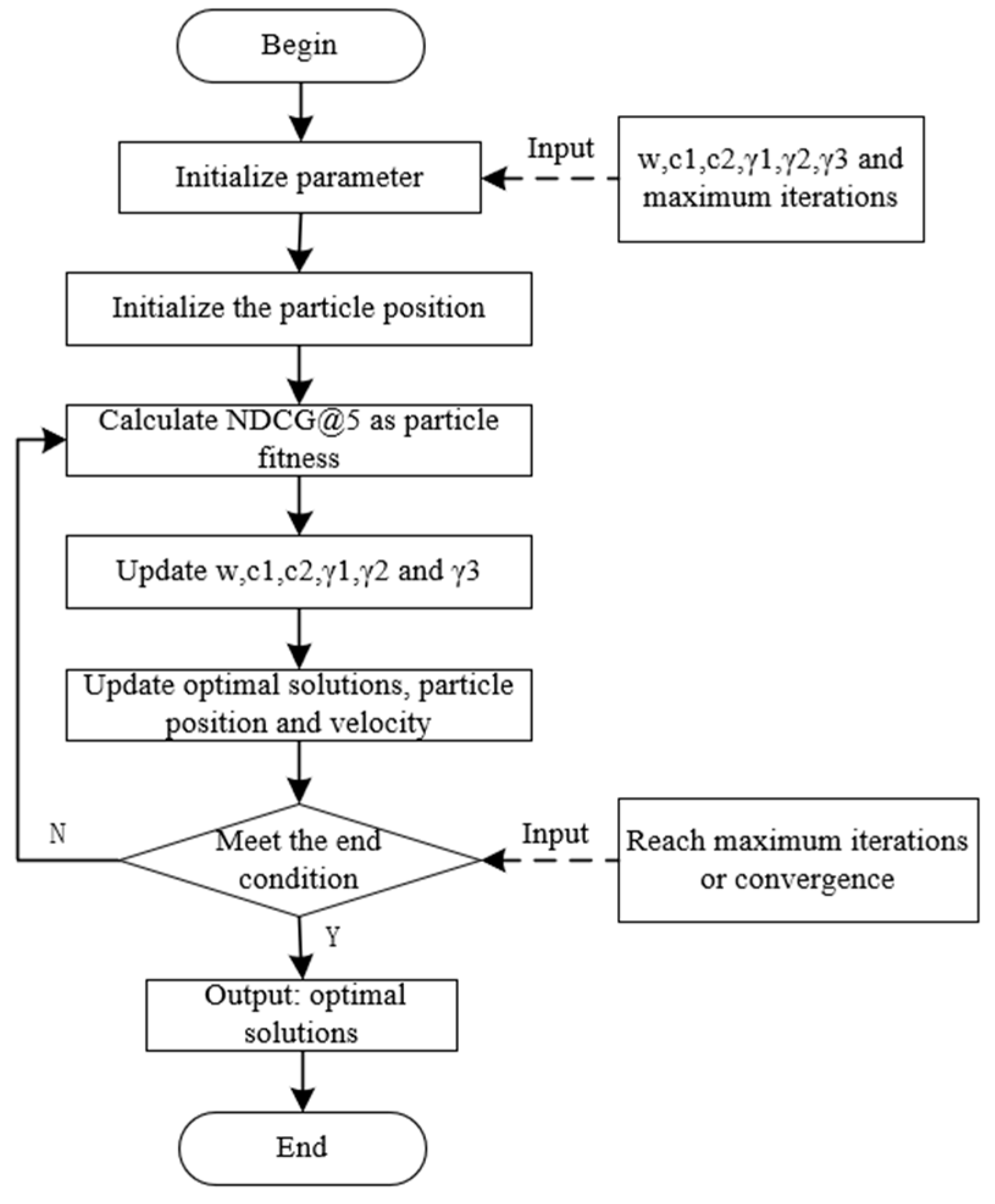
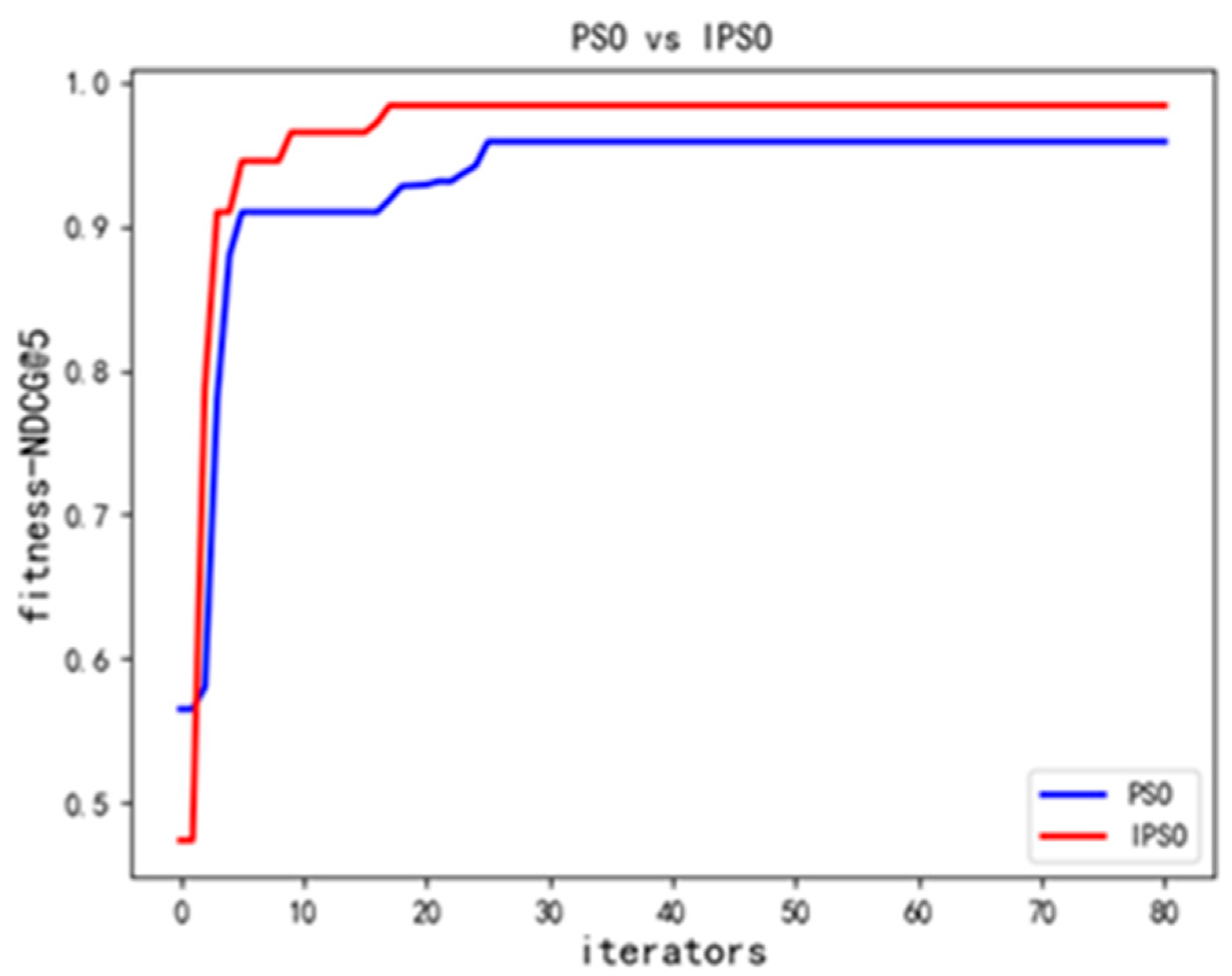
3.2.2. Parameter Optimization

The IPSO is proposed to change the inertia weight w, and learning factors c1 and c2 in the original PSO algorithm to adjust the coefficient weights γ1, γ2, and γ3 in Formula (9) to find the optimal weights for precipitation image retrieval. IPSO changes the above three parameters adaptively with the increase in the number of iterations to avoid the algorithm falling into the partial optimal solution. The major improvements in IPSO include:
  • Inertia weight w;
Parameter w represents the degree of retention of the particle to the speed of the last iteration, which can adjust the global and local search capabilities of the algorithm. The larger w takes at the early stage of the iteration, the stronger the particle global search ability is. The smaller w takes at the later stage of the iteration, the stronger the particle local search ability is. Therefore, IPSO takes the strategy of decreasing the number of iterations k linearly to balance the global and local search capabilities of particles, where the relationship between w and the number of iterations k is represented as follows:
w ( k ) = w m a x ( w m a x w m i n ) k m a x k k m a x
where wmax is the initial maximum inertia weight, wmin is the minimum inertia weight when iterating to the maximum algebra, kmax is the maximum number of iterations, and w(k) is the inertia weight value when iterating for k times.
  • Learning ratio c1 and c2;
Parameters c1 and c2 represent the ability of a particle to learn from the individual and the group optimal solution, respectively, and usually take the same value between 0 and 4 based on experience. Moreover, if c1 takes a large value and c2 takes a small value in the early stages of the iteration it can enhance the global search ability of the particles. Meanwhile, if c1 takes a small value and c2 takes a large value in the later stages of the iteration, it can improve the local search ability of particles. Therefore, IPSO improves parameters c1 and c2 with the symmetric linear strategy [27] to optimize the learning ability of individual optimal solutions and group optimal solutions for particles. The improvements in c1 and c2 are presented as follows:
c 1 . b e g i n = c 2 . e n d = c m i d   + Δ c
c 2 . b e g i n = c 1 . e n d = c m i d   Δ c
c 1 ( k ) = c 1 . b e g i n k k m a x ( c 1 . b e g i n c 1 . e n d ) = c m i d   + Δ c ( 1 2 k k m a x )
c 2 ( k ) = c 2 . b e g i n k k m a x ( c 2 . e n d c 2 . b e g i n ) = c m i d   Δ c ( 1 2 k k m a x )
where c1.begin and c1.end represent the initial and termination values of c1, so do c2.begin and c2.end. ∆c represents the maximum variable length of c1 and c2; cmid is the middle value of c1 and c2.

4. Experiment and Result Analysis

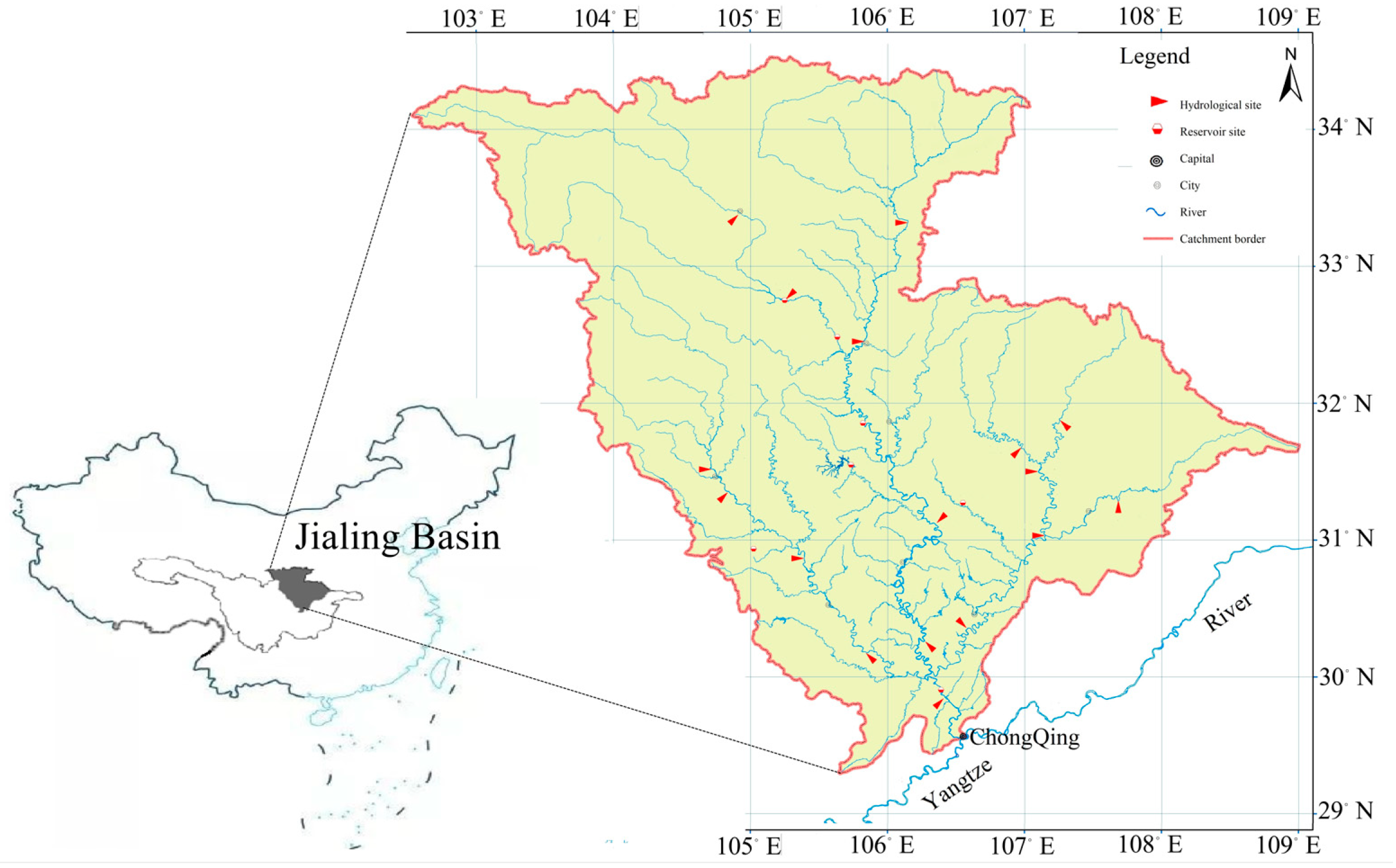
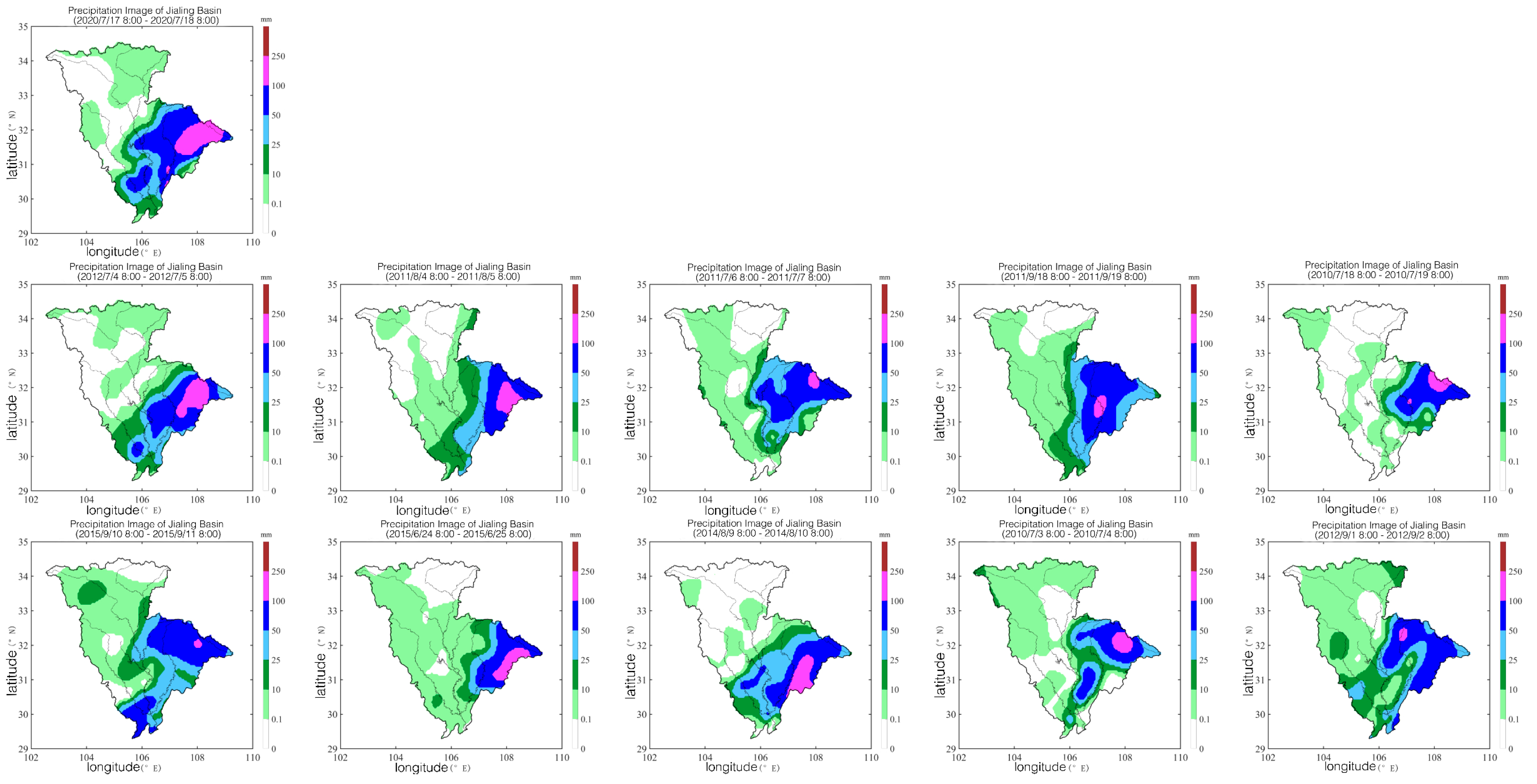
4.1. Study Area and Data Preprocessing

The Jialing River is the largest branch of the Yangtze River, which is about 1120 km long and covers an area of approximately 160,000 square kilometers within a geographical range of 29°17′30″ N–34°28′11″ N and 102°35′36″ E–109°01′08″ E (Figure 6). It belongs to the humid monsoon climate region, with an average annual precipitation of 931 mm. In normal years, the floods caused by rainfall in the basin are mostly concentrated in July and August with the characteristics of rapid fluctuation, short duration, fast flow rate, and high flood peak, which pose a great threat to the life and property of the residents along the river.
To verify the NDCG-IPSO method for image similarity search, daily precipitation images from Jialing Basin from 1 January 2010, to 12 December 2019, were used for training and validation. Therefore, the experiment chose 30 precipitation images with different rainfall grades (6 images of light rain, 9 images of moderate rain, and 15 images of heavy rain) as the query samples and 10 matching samples for each query sample from the historical precipitation image. Additionally, each matching sample was assigned a similarity score from 0 (totally dissimilar) to 2 (very similar) according to expert experience to measure how similar the query sample and the matched sample were. In the experiment, the query samples were divided into the training sample set and test sample set according to the ratio of 2:1.

4.2. Results Analysis

The NDCG-IPSO was used to conduct image similarity search experiments on the daily precipitation images of the Jialing Basin. γ1, γ2, and γ3 were initialized randomly, and their sum was guaranteed to be 1. The inertia weight w was set to 0.9, which linearly decreases to 0.4 as the number of iterations increases according to the Formula (13). Individual learning factors c1 and social learning factors c2 were set at 2.5 and 1.25. The particle number and the iteration number of the IPSO were set to 30 and 80 to obtain the optimal parameters of multi-feature distances for the precipitation image, which was shown in Table 1.
Therefore, we adopted γ1= 0.46, γ2= 0.12, and γ3 = 0.42 to calculate the comprehensive distance between precipitation images in subsequent experiments. The experimental results using indicators NDCG@5 and NDCG@10 were shown in Table 2.
As seen in Table 2, the NDCG-IPSO can obtain higher index values on both training and test samples. Particularly, the average accuracy of NDCG@5 and NDCG@10 of the method on the test samples were 0.978 and 0.964, respectively, which were very close to 1. The experimental results prove the following two points: On the one hand, the three features extracted in this paper can well represent the spatial and temporal characteristics of the precipitation image and meet the needs of the precipitation image analysis, which can be used as indicators for image similarity of daily precipitation images. On the other hand, the NDCG-IPSO has a good effect on fusing feature distances defined in this paper into the comprehensive distance and thus quickly retrieves similar images from precipitation images.
Figure 7 shows the similarity search results of the precipitation image based on the NDCG-IPSO. For the precipitation image to be queried in the first line shown in Figure 7, lines 2 and 3 display the top 10 images that are very similar in terms of regional precipitation, precipitation distribution, and precipitation center, which can prove the effectiveness of this method and provide technical support for the analysis of similar hydrological processes.

4.3. Comparative Analysis

To further verify the applicability and robustness of NDCG-IPSO, this experiment compared the image search results of our method with color histogram (CH) [28,29], BORDA [30], principal component analysis (PCA) [31], and the NDCG-PSO under the same conditions. Table 3 shows the image search results of the five methods on the same dataset.
A color histogram is widely used in many image retrieval systems, which search similar images by extracting color histograms in images and calculating the distance between the histograms. Considering that precipitation images mainly adopt color features to represent different precipitation information, the color histogram is perhaps the most suitable method for precipitation image similarity searches. The global CH [28] and the block CH [29] with 3 × 3 blocks are used to search similar precipitation images. The results shown in Table 3 indicate that though global CH it can well characterize the color features of precipitation images, it ignores the spatial information of color features and results in low accuracy of similarity retrieval. The block CH considers part of the spatial information, and its searching accuracy is better than that of the global CH. However, block CH does not consider the physical meaning of the different colors on the precipitation image, which leads to worse searching accuracy than that of NDCG-IPSO.
The PCA and BORDA are two commonly used multi-index comprehensive evaluation methods, which are also widely used in the mining of multivariate hydrological similarity. The PCA conducts principal component analysis on all three feature distances and takes the feature with cumulative variance contribution rates greater than 85% as the principal component, and then weighs the features according to their variance contribution rates to obtain the search results after sorting. The BORDA sorts the feature distance once and synthesizes the similarity search results of those feature distances by BORDA to obtain the final query result. Although PCA, BORDA and NDCG-IPSO extract precipitation spatial distribution, precipitation center, and regional precipitation and comprehensively consider three distances to search similar images, NDCG-IPSO uses machine learning algorithms to optimize ensemble weighing method parameters and thus achieves better results than that of PCA and BORDA.
The only difference between NDCG-PSO and NDCG-IPSO is that the latter adopts the inertia weight and two learning factors in the PSO algorithm with an increase in the number of iterations. This adaptive adjustment improves the search performance and accuracy of the NDCG-IPSO. Figure 8 shows the fitness function value, namely NDCG@5, varying with the number of iterations in the NDCG-PSO and NDCG-IPSO. It can be seen from Figure 8 that NDCG-IPSO obtains the optimal particle fitness of 0.984 after 18 iterations; while NDCG-PSO gets stuck in a local optimum of 0.959 after 27 iterations. This indicates that IPSO can improve the search accuracy and optimization speed of image similar search and thus provides support for improving similar precipitation image retrieval.

5. Conclusions

This paper proposes a rainfall similarity research method based on deep learning by using precipitation images. Firstly, the regional precipitation, precipitation distribution, and precipitation center are extracted from the precipitation images, and the similarity measurement for each feature is calculated separately.
Additionally, an ensemble weighting method of normalized depreciation cumulative gain-improved particle swarm optimization (NDCG-IPSO) is proposed to weigh and fuse the three extracted features as the similarity measure of the precipitation image. Finally, the comparing experiment of our method with CH, PCA, BORDA, and NDCG-PSO on the daily precipitation images in the Jialing River Basin illustrates that the methods proposed in this paper can better characterize the spatiotemporal characteristics of the precipitation image and discover similar rainfall processes, which will provide a new idea for hydrological forecasting.
Although some achievements have been made, many problems must still be solved. One problem is that it only considers the daily precipitation images similarity searching. However, a rainfall process may be composed of multiple single-day precipitation images.
Hence, how to conduct the rainfall process similarity search based on the similarity measurement method of NDCG-PSO and thus build a rainfall-flood similarity pattern repository to provide guidance and technical support for hydrological forecasting and water resource utilization is the direction of our future work.

Author Contributions

Conceptualization, Y.Y.; Methodology, Y.Y., X.H., Y.Z. and D.W.; Software, X.H.; Validation, Y.Z.; Formal analysis, X.H.; Writing—original draft, X.H.; Writing—review & editing, Y.Y. and D.W.; Visualization, X.H.; Supervision, Y.Y., Y.Z. and D.W.; Project administration, Y.Y., Y.Z. and D.W. All authors have read and agreed to the published version of the manuscript.

Funding

This research was funded by the National Key R&D Program of China (No. 2021YFB3900605 and 2018YFC1508100).

Institutional Review Board Statement

Not applicable.

Informed Consent Statement

Not applicable.

Data Availability Statement

Not applicable.

Acknowledgments

The authors would like to thank the Bureau of Hydrology, Changjiang water Resources Commission, especially Chen Yubin and Zhang Xiao, for their great help in data provision, algorithm design, and model training of this paper.

Conflicts of Interest

The authors declare no conflict of interest.

References

  1. Li, B.; Liang, Z.; Bao, Z.; Wang, J.; Hu, Y. Changes in streamflow and sediment for a planned large reservoir in the middle Yellow River. Land Degrad. Dev. 2019, 30, 878–893. [Google Scholar] [CrossRef] [Green Version]
  2. Stenta, H.R.; Riccardi, G.A.; Basile, P.A. Grid size effects analysis and hydrological similarity of surface runoff in flatland basins. Hydrol. Sci. J. 2017, 62, 1736–1754. [Google Scholar] [CrossRef]
  3. Liang, Z.; Xiao, Z.; Wang, J.; Sun, L.; Li, B.; Hu, Y.; Wu, Y. An improved chaos similarity model for hydrological forecasting. J. Hydrol. 2019, 577, 123953. [Google Scholar] [CrossRef]
  4. Dilmi, D.; Barthès, L.; Mallet, C.; Aymeric, C. Modified DTW for a quantitative estimation of the similarity between rainfall time series. EGU Gen. Assem. 2017, 19, EGU2017-16005. [Google Scholar]
  5. Xiao, Z.; Liang, Z.; Li, B.; Hou, B. New flood early warning and forecasting method based on similarity theory. J. Hydrol. Eng. 2019, 24, 04019023. [Google Scholar] [CrossRef] [Green Version]
  6. Barthel, R.; Haaf, E.; Giese, M.; Nygren, M.; Heudorfer, B.; Stahl, K. Similarity-based approaches in hydrogeology: Proposal of a new concept for data-scarce groundwater resource characterization and prediction. Hydrogeol. J. 2021, 29, 1693–1709. [Google Scholar] [CrossRef]
  7. Wang, H.; Xing, C.; Yu, F. Study of the hydrological time series similarity search based on Daubechies wavelet transform. In Unifying Electrical Engineering and Electronics Engineering, Proceedings of the 2012 International Conference on Electrical and Electronics Engineering, London, UK, 4–6 July 2012; Springer: New York, NY, USA, 2013; pp. 2051–2057. [Google Scholar]
  8. Yang, J.; Wan, D.; Yu, Y. Similarity Search Method of Hydrological Time Series based on Fragment Alignment Distance and Dynamic Time Warping. In Proceedings of the IEEE 2022 5th International Conference on Advanced Electronic Materials, Computers and Software Engineering (AEMCSE), Wuhan, China, 22–24 April 2022; pp. 214–220. [Google Scholar]
  9. Zhang, L.; Zhu, Y.; Li, S.; Gao, X. Study on Similarity Model of Precipitation Series Based on Precipitation Type Histogram. J. China Hydrol. 2013, 33, 10–16. [Google Scholar]
  10. Ohno, G.; Kazunori, I. Flood Forecast Based on Deep Learning Using Distribution MAP of Precipitation. In Proceedings of the 22nd IAHR APD Congress, Sapporo, Japan, 14–17 September 2020. [Google Scholar]
  11. Wang, X.; Liu, Y.; Chen, Y.; Liu, Y. An adaptive density-based time series clustering algorithm: A case study on rainfall patterns. ISPRS Int. J. Geo-Inf. 2016, 5, 205. [Google Scholar] [CrossRef] [Green Version]
  12. Gang, J.; Zhao, W. RETRACTED ARTICLE: Remote sensing image-based rainfall changes in plain areas and IoT motion image detection. Arab. J. Geosci. 2021, 14, 1–17. [Google Scholar] [CrossRef]
  13. Pradhan, J.; Kumar, S.; Pal, A.K.; Banka, H. Texture and colour region separation based image retrieval using probability annular histogram and weighted similarity matching scheme. IET Image Process. 2020, 14, 1303–1315. [Google Scholar] [CrossRef]
  14. Wu, Y.; Zhang, L.; Berretti, S.; Wan, S. Medical Image Encryption by Content-Aware DNA Computing for Secure Healthcare. IEEE Trans. Ind. Inform. 2023, 19, 2089–2098. [Google Scholar] [CrossRef]
  15. Divakar, R.; Singh, B.; Bajpai, A.; Kumar, A. Image pattern recognition by edge detection using discrete wavelet transforms. J. Decis. Anal. Intell. Comput. 2022, 2, 26–35. [Google Scholar]
  16. Alsmadi, M.K. Content-based image retrieval using color, shape and texture descriptors and features. Arab. J. Sci. Eng. 2020, 45, 3317–3330. [Google Scholar] [CrossRef]
  17. Kumbure, M.M.; Luukka, P. A generalized fuzzy k-nearest neighbor regression model based on Minkowski distance. Granul. Comput. 2022, 7, 657–671. [Google Scholar] [CrossRef]
  18. Gassouma, M.S.; Benhamed, A.; El Montasser, G. Investigating similarities between Islamic and conventional banks in GCC countries: A dynamic time warping approach. Int. J. Islam. Middle East. Financ. Manag. 2023, 16, 103–129. [Google Scholar] [CrossRef]
  19. Ristad, E.S.; Yianilos, P.N. Learning String-Edit Distance. IEEE Trans. Pattern Anal. Mach. Intell. 1997, 20, 522–532. [Google Scholar] [CrossRef] [Green Version]
  20. Benti, N.E.; Chaka, M.D.; Semie, A.G. Forecasting Renewable Energy Generation with Machine learning and Deep Learning: Current Advances and Future Prospects. Preprints.org 2023, 2023030451. [Google Scholar] [CrossRef]
  21. Zhang, L.; Zhang, B. Deep learning for remote sensing data: A technical tutorial on the state of the art. IEEE Geosci. Remote Sens. Mag. 2016, 4, 22–40. [Google Scholar] [CrossRef]
  22. Frana, R.P.; Monteiro, A.; Arthur, R.; Lano, Y. An overview of deep learning in big data, image, and signal processing in the modern digital age. Trends Deep. Learn. Methodol. 2021, 63–87. [Google Scholar] [CrossRef]
  23. Wu, Y.; Guo, H.; Chakraborty, C.; Khosravi, M.; Berretti, S.; Wan, S. Edge Computing Driven Low-Light Image Dynamic Enhancement for Object Detection. IEEE Trans. Netw. Sci. Eng. 2022, 3151502. [Google Scholar] [CrossRef]
  24. Kennedy, J.; Eberhart, R. Particle swarm optimization. In Proceedings of the ICNN’95-International Conference on Neural Networks, Perth, WA, Australia, 27 November–1 December 1995; Volume 4, pp. 1942–1948. [Google Scholar]
  25. Paramanik, A.R.; Sarkar, S.; Sarkar, B. OSWMI: An Objective-Subjective Weighted method for Minimizing Inconsistency in multi-criteria decision making. Comput. Ind. Eng. 2022, 169, 108138. [Google Scholar] [CrossRef]
  26. Furui, K.; Ohue, M. Compound virtual screening by learning-to-rank with gradient boosting decision tree and enrichment-based cumulative gain. In Proceedings of the 2022 IEEE Conference on Computational Intelligence in Bioinformatics and Computational Biology (CIBCB), Ottawa, ON, Canada, 15–17 August 2022; pp. 1–7. [Google Scholar]
  27. Feng, K.; Li, X.; Qian, X.; Wu, L.; Zheng, H.; Chen, M.; Li, M.; Liu, B. Atmospheric Optical Turbulence Profile Model Fitting Based on Improved Particle Swarm Algorithm. Laser Optoelectron. Prog. 2022, 59, 73–84. [Google Scholar]
  28. Liu, C.; Sui, X.; Kuang, X.; Liu, Y.; Gu, G.; Chen, Q. Optimized Contrast Enhancement for Infrared Images Based on Global and Local Histogram Specification. Remote Sens. 2019, 11, 849. [Google Scholar] [CrossRef] [Green Version]
  29. Li, K.; Sun, X.; Gao, B.; Zhou, J. Weighted Histogram Block Detection Algorithm for Digital Trunking Terminal. In Proceedings of the International Conference on Intelligent Automation and Soft Computing, Chicago, IL, USA, 28–30 May 2021; Springer: Cham, Switzerland, 2021; pp. 166–172. [Google Scholar]
  30. Muhammad, M.; Oscar, V. Pairwise consensus and the Borda rule. Math. Soc. Sci. 2022, 116, 17–21. [Google Scholar]
  31. Boudou, A.; Viguier-Pla, S. Principal components analysis and cyclostationarity. J. Multivar. Anal. 2022, 189, 104875. [Google Scholar] [CrossRef]
Figure 1. Example of precipitation image.
Applsci 13 04883 g001
Figure 2. The process flow of precipitation image searching.
Applsci 13 04883 g002
Figure 3. The precipitation distribution matrix.
Applsci 13 04883 g003
Figure 4. The distance between RA(i, j) and RB(i, j) of two precipitation distribution matrixes.
Applsci 13 04883 g004
Figure 5. Flow chart of NDCG-IPSO.
Applsci 13 04883 g005
Figure 6. Location of the Jialing Basin.
Applsci 13 04883 g006
Figure 7. Image search results of NDCG-IPSO.
Applsci 13 04883 g007
Figure 8. Comparison of experimental results between PSO algorithm and IPSO algorithm.
Applsci 13 04883 g008
Table 1. Optimal weights of the three feature distances for precipitation image.
Feature Distanceγ1γ2γ3
coefficient0.460.120.42
Table 2. Optimal weights of the three feature distances for precipitation image.
AccuracyNDCG@5NDCG@10
Images
Training sample 0.9840.978
Test sample 0.9780.964
Table 3. Comparative analysis of image search results based on different methods.
AccuracyNDCG@5NDCG@10
Method
NDCG-IPSO0.9780.964
Global CH [28]0.7210.662
Block CH [29]0.8340.803
BORDA [30]0.8360.796
PCA [31]0.7020.623
NDCG-PSO0.9590.923
Disclaimer/Publisher’s Note: The statements, opinions and data contained in all publications are solely those of the individual author(s) and contributor(s) and not of MDPI and/or the editor(s). MDPI and/or the editor(s) disclaim responsibility for any injury to people or property resulting from any ideas, methods, instructions or products referred to in the content.

