Fault Prediction of Mechanical Equipment Based on Hilbert–Full-Vector Spectrum and TCDAN

Abstract

To solve the problem of “under-maintenance” and “over-maintenance” in the daily maintenance of equipment, the predictive maintenance method based on the running state of equipment has shown great advantages, and fault prediction is an important part of predictive maintenance. First, the spectrum information of the equipment is extracted by the Hilbert–full-vector spectrum as the input of fault prediction. Compared with the traditional spectrum, this spectrum information fuses the signals of two sensors in the same section of the device, which can reflect the actual operational state of the device more comprehensively. Then, the temporal convolutional network is used to predict the amplitudes of different feature frequencies, and the double-layer attention mechanism is introduced to mine the correlation between the corresponding amplitudes of different feature frequencies and between the data at different historical moments, to highlight the more important influencing factors. In this way, the prediction accuracy of the model for the amplitude corresponding to the feature frequency of concern is improved. Finally, experimental verification is carried out on the XJTU-SY dataset. The results show that the TCDAN model proposed in this paper is significantly superior to TCN, GRU, BiLSTM, and LSTM, which can provide a more effective decision-making basis for the predictive maintenance of equipment.

1. Introduction

With the development of industrialization, mechanical equipment has been widely used in all walks of life. There are many parts and components of mechanical equipment, and most of the equipment is in the state of frequent startup or continuous operation in the work. Various faults inevitably occur during the use of the equipment. When faults occur, they may affect normal production or even cause safety concerns. If the occurrence of equipment failure can be accurately predicted, to take targeted measures in advance, many uncontrollable risks will be avoided [1]. Therefore, it is of great practical significance to realize the fault prediction of equipment [2].

For equipment fault prediction, it is mainly divided into the method based on the mechanism model, the method based on data-driven, and the method combining the two [3,4,5,6]. Based on the mechanism model, the degradation model is established based on an in-depth analysis of the failure mechanism of the equipment [7]. Because the specific mechanism model of the device is almost difficult to build, it is not widely used.

The data-driven method is mainly based on the historical operational data of the equipment to mine the change rule [8], to predict the faults of the equipment. To date, it has been widely studied by many scholars, such as the autoregressive model [9], the gray prediction model [10], support vector regression (SVR) [11,12], the artificial neural network (ANN) [13] and other methods are used in the fault-tendency prediction or the remaining useful life prediction of mechanical equipment. With the development of artificial intelligence technology, Recurrent Neural Network (RNN) [14,15], Long Short-Term Memory (LSTM) [16,17], Bidirectional Long Short-term Memory (BiLSTM) [18,19], Gate Recurrent Unit (GRU) [20,21] and other models have been used in fault-tendency prediction and remaining useful life prediction with their powerful time-series processing ability, and have achieved better results [8]. However, LSTM, BiLSTM, and GRU are still RNN structures in essence. Although the gradient explosion and disappearance problems in RNN have been alleviated, parallel computing still cannot be carried out.

Bai et al. proposed the temporal convolutional network (TCN) model [22], which is different from the structure of RNN and does not have the problem of gradient explosion and disappearance. At the same time, due to the introduction of the shared convolution kernel, the model can carry out parallel calculation, which effectively improves the speed of model calculation. The prediction effect in multiple tasks has exceeded that of LSTM and GRU and other recurrent neural network structures, providing a new idea for the processing of time-series tasks [22,23,24,25]. However, the single temporal convolutional network ignores the correlation between different dimensions of data. Since the attention mechanism has achieved good results in measuring the importance of input features, the double-layer attention mechanism [26,27,28] was introduced based on the temporal convolutional network model. The introduced attention layer is used to mine the correlation between different input features and data at different historical moments, respectively. By increasing the weight of the corresponding parameters, the factors that have a greater impact on the prediction value in the input of the model are highlighted.

On the other hand, the current fault-prediction research mainly focuses on fault-tendency prediction and the remaining useful life prediction of mechanical equipment. The prediction results cannot reflect the specific information of the type of equipment fault. In this paper, based on the traditional Hilbert-envelope spectrum [11,29,30], combined with full-vector spectrum [31,32] technology, the dual-channel vibration data of the equipment are fused to obtain the spectrum information that can fully reflect the running state of the equipment, which is used as the fault-prediction feature.

2. Fault Feature Extraction

With the development of equipment precision, to ensure the reliability and integrity of signal acquisition, multiple identical sensors are often used for the signal acquisition of a certain part of the equipment at the same time. In addition, sensors are generally arranged in the horizontal–vertical direction or V-shaped direction in the same plane, as shown in Figure 1.

The Hilbert-envelope spectrum mainly uses the Hilbert transformation to demodulate the amplitude of the original vibration signal of the equipment, removes the high-frequency vibration component, realizes the envelope demodulation of the signal, and has great advantages in extracting fault features [29,30]. The processing flow is shown in Figure 2a. The traditional Hilbert-envelope spectrum can only process and analyze the signals collected by multiple sensors separately, and the signals collected by a single sensor are not comprehensive enough, which leads to one-sided analysis results. In this paper, full-vector spectrum technology is introduced based on the traditional Hilbert-envelope spectrum, and information fusion is carried out after envelope processing for the signals collected in the two directions of the device. Finally, FFT (Fast Fourier Transform) operation is performed to obtain more comprehensive spectrum information on the device. The processing flow is shown in Figure 2b.

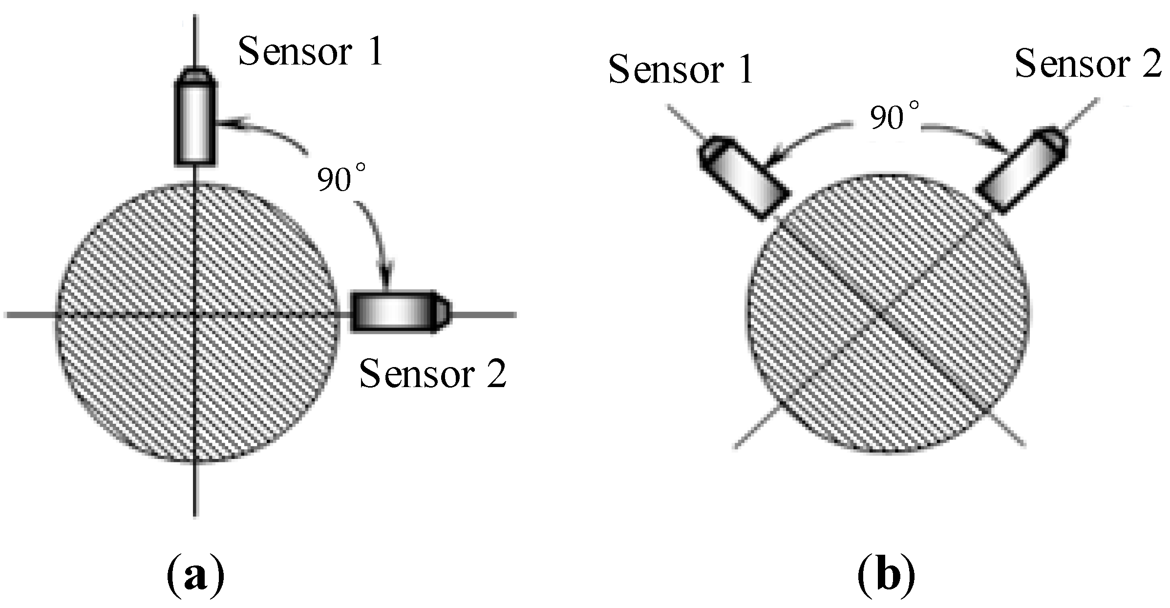
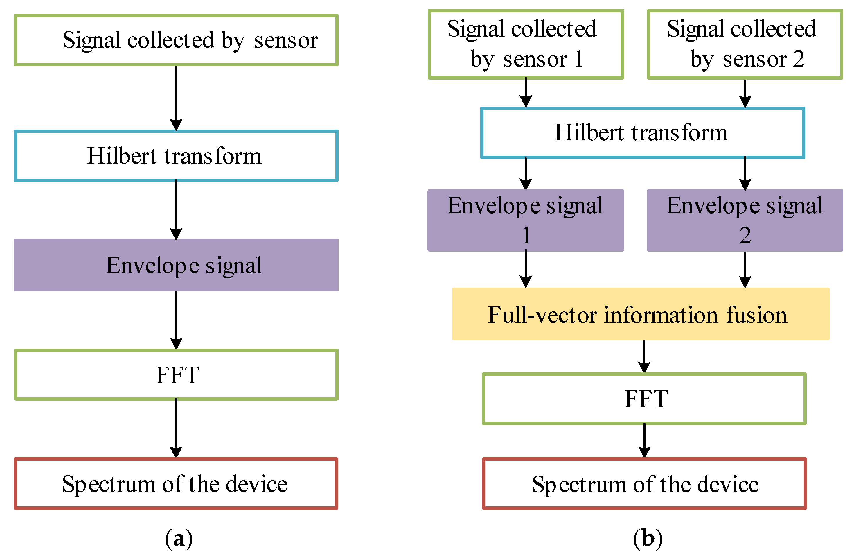
2.1. Hilbert-Envelope Spectrum

The principle of signal enveloping using the Hilbert transform is to first make the original signal generate a 90° phase shift, to form an analytical signal with the original signal [29,30]. Let $S\left(t\right)$ be a real signal, and its Hilbert transformation is defined as:

$$S_h\left(t\right)=S\left(t\right)\ast \frac{1}{\pi t}=\frac{1}{\pi }{{\displaystyle \int }}_{-\infty }^{+\infty }\frac{S\left(\tau \right)}{t-\tau }\mathrm{d}\tau$$

(1)

where $\ast$ indicates the convolutional calculation. Then, the original signal $S\left(t\right)$ and its Hilbert transformation signal $S_h\left(t\right)$ can constitute an analytical signal $S_a\left(t\right)$:

$$S_a\left(t\right)=S\left(t\right)+j{S}_h\left(t\right)$$

(2)

Its amplitude $A\left(t\right)$:

$$A\left(t\right)=\sqrt{S^2\left(t\right)+S_h^2\left(t\right)}$$

(3)

$A\left(t\right)$ is the envelope of the real signal $S\left(t\right)$. Then the Hilbert-envelope spectrum of the original signal can be obtained by FFT operation on the envelope signal.

2.2. Full-Vector Spectrum

Suppose $\left\{H_i\right\}$ and $\left\{V_i\right\}$ are discrete sequences in the horizontal and vertical directions, respectively. To further improve the computational efficiency, the sequences $\left\{H_i\right\}$ and $\left\{V_i\right\}$ constitute complex sequences:

$$\left\{z_i\right\}=\left\{H_i\right\}+j\left\{V_i\right\}\left(i=1,2,\dots ,\mathrm{N}/2-1\right)$$

(4)

By Fourier transform, it becomes:

$$\left\{Z_i\right\}=\left\{Z_{Ri}\right\}+\left\{Z_{Ii}\right\}$$

(5)

where $Z_{Ri}$, $Z_{Ii}$ are the real and imaginary parts of Z_i, respectively.

According to the definition of full-vector spectrum theory [31,32], the major half-axis of the elliptic trajectory of the rotor under a certain harmonic is called the principal vector of the harmonic, which is expressed by $R_{ai}$. The minor semi-axis is called the auxiliary oscillator vector under the harmonic, denoted by $R_{bi}$, and thus the following can be obtained:

$$\begin{array}{cc}{R}_{ai}& =\frac{1}{2N}\left[\left|Z_i\right|+\left|Z_{\left(N-i\right)}\right|\right]\\ R_{bi}& =\frac{1}{2N}\left[\left|Z_i\right|+\left|Z_{\left(N-i\right)}\right|\right]\\ \tan 2{\alpha }_i& =\frac{Z_{Ii}{Z}_{R\left(N-i\right)}-Z_{Ri}{Z}_{I\left(N-i\right)}}{Z_{Ri}{Z}_{R\left(N-i\right)}+Z_{Ii}{Z}_{I\left(N-i\right)}}\\ \tan {\varphi }_i& =\frac{Z_{Ii}+Z_{\left(N-i\right)}}{Z_{Ri}+Z_{R\left(N-i\right)}}\\ (i& =1,2,\cdots ,N/2-1)\end{array}$$

(6)

where ${\alpha }_i$ is the angle between the principal oscillator vector and the horizontal direction, and ${\varphi }_i$ is the phase angle when the axis moves along the elliptic trajectory.

2.3. Hilbert–Full-Vector Spectrum

The traditional Hilbert-envelope spectrum is based on the Fourier transform of the envelope signal of a single channel, and the obtained device spectrum information is not comprehensive. The Hilbert–full-vector spectrum is based on the principle of homologous information fusion. First, the Hilbert-envelope signals of the horizontal and vertical channels at the same section of the device are fused, and then FFT operation is performed to obtain the spectrum information that can fully reflect the actual state of the device. The steps of the Hilbert–full-vector spectrum are as follows:

(1) Two identical sensors are used to simultaneously collect signals, $H\left(t\right)$, $V\left(t\right)$, from the mutual perpendicular direction of the same section of the rotating device.

(2) According to Equations (1) and (2), the Hilbert transform is applied to signals H(t) and $V\left(t\right)$ to obtain $H_h\left(t\right)$ and $V_h\left(t\right)$, respectively, thus constituting analytic signals $H_a\left(t\right)$ and $V_a\left(t\right)$ with the original signals $H\left(t\right)$ and $V\left(t\right)$:

$$\begin{array}{c} H_a\left(t\right)=H\left(t\right)+j{H}_h\left(t\right)\\ V_a\left(t\right)=V\left(t\right)+j{V}_h\left(t\right)\end{array}$$

(7)

Then the envelopes of $H\left(t\right)$ and $V\left(t\right)$ are obtained according to Equation (3) as follows:

$$\begin{array}{c}{A}_H\left(t\right)=\sqrt{H^2\left(t\right)+H_h^2\left(t\right)}\\ A_V\left(t\right)=\sqrt{V^2\left(t\right)+V_h^2\left(t\right)}\end{array}$$

(8)

(3) Based on the full vector spectrum technology, the dual-channel envelope signals $A_H\left(t\right)$ and $A_V\left(t\right)$ are fused with the same source information, and the principal vector is obtained by Equations (4)–(6), and then the FFT operation is performed on it. Finally, the spectrum information that can reflect the actual operational state of the device is obtained.

3. Construction of Prediction Model

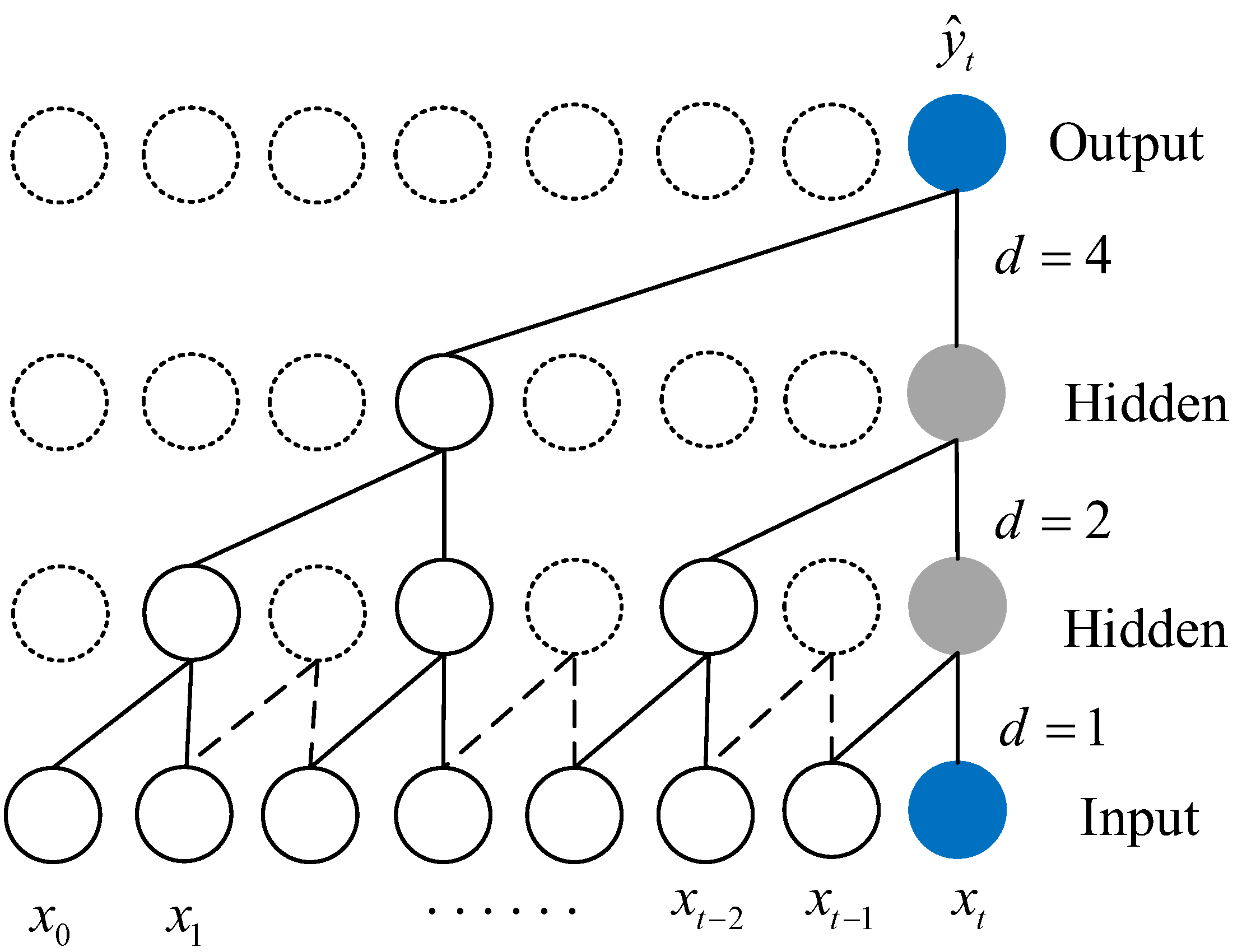
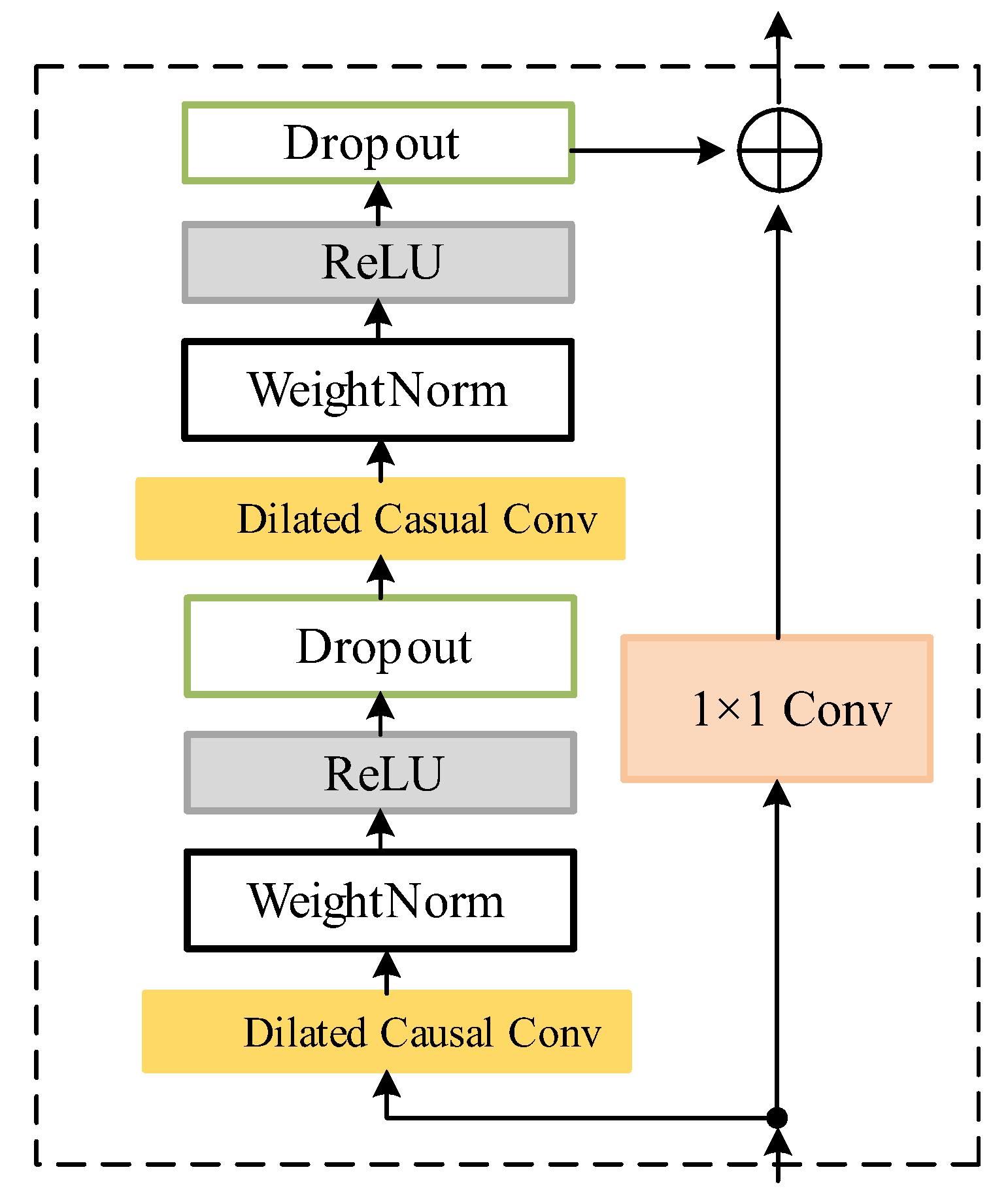
The prediction effect of TCN on multiple tasks has surpassed that of recurrent neural network structures such as LSTM and GRU, which provides a new idea for the processing of time-series tasks. However, a single temporal convolutional network ignores the correlation between different dimensions of data. Since the attention mechanism has achieved good results in measuring the importance of input features, the two-layer attention mechanism is introduced based on the temporal convolutional network model. The prediction accuracy of the model is improved by highlighting the factors in the input that have a greater impact on the predicted value.

3.1. TCN Model

TCN is a model that uses a convolutional structure to solve time-series problems and mainly consists of dilated causal convolution and residual modules [22]. TCN uses causal convolution to ensure that there is no information leakage. Suppose that the model input sequence is {x₀, x₁ … x_t-1, x_t}, the expected prediction output is {y₀, y₁ … y_t-1, y_t}. In causal convolution, the output predicted value ${\widehat{y}}_t$ at time t is only determined by {x₀, x₁ … x_t-1, x_t}, independent of {x_t+1, x_t+2 …}. To capture long-timescale dependence in the time-series, dilated convolution is introduced into the causal convolution to become the dilated causal convolution that can realize the exponential increase of the receptive field, and the structure is shown in Figure 3.

For a one-dimensional input sequence $x\in {\mathrm{R}}^n$ and a filter f: {0,1,…, k − 1} → R, the dilated convolution operation F on the sequence element s is defined as follows:

$$F\left(s\right)={\sum }_{i=0}^{k-1}f\left(i\right)·x_{s-d·i}$$

(9)

where k is the size of the convolution kernel, d is the dilation factor, and $x_{s-d·i}$ represents the element of the historical moment in the input sequence.

The larger the dilation factor d, the larger the input range, thus increasing the receptive field of the convolutional network. As shown in Figure 2, the dilated causal convolution is one with dilation factor $d$ = {1,2,4}, convolution kernel size $k$ = 2, and final receptive field size 8.

With the superposition of dilated causal convolutions, the depth of the network will be deepened, which may lead to the problem of gradient disappearance in the model. Therefore, a residual connection is introduced in the output layer of TCN to fuse the input $x$ into the output of the convolutional network, which can be expressed as follows:

$$o=\mathrm{Activation}\left(x+F\left(x\right)\right)$$

(10)

where Activation (·) is the activation function and $F\left(x\right)$ represents the output of the convolutional layer.

After the introduction of a residual connection in TCN, as shown in Figure 4, a residual connection can make the deeper network work properly, which can improve the performance of the model [33]. The WeightNorm layer normalizes the weight of the output of the convolutional layer to speed up the calculation [34]. Meanwhile, to avoid overfitting, a Dropout layer is added after each dilated causal convolution.

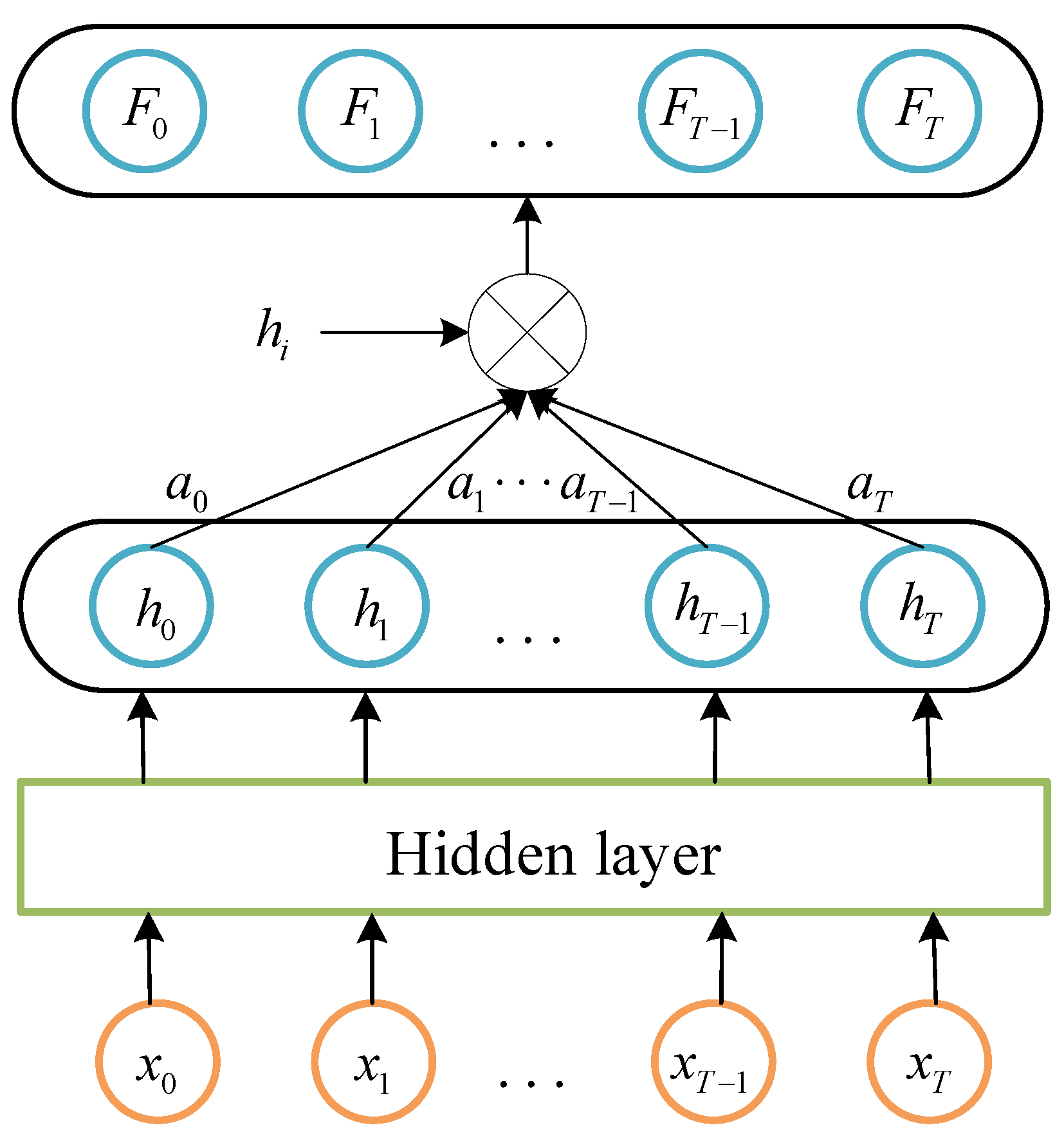
3.2. Attention Mechanism

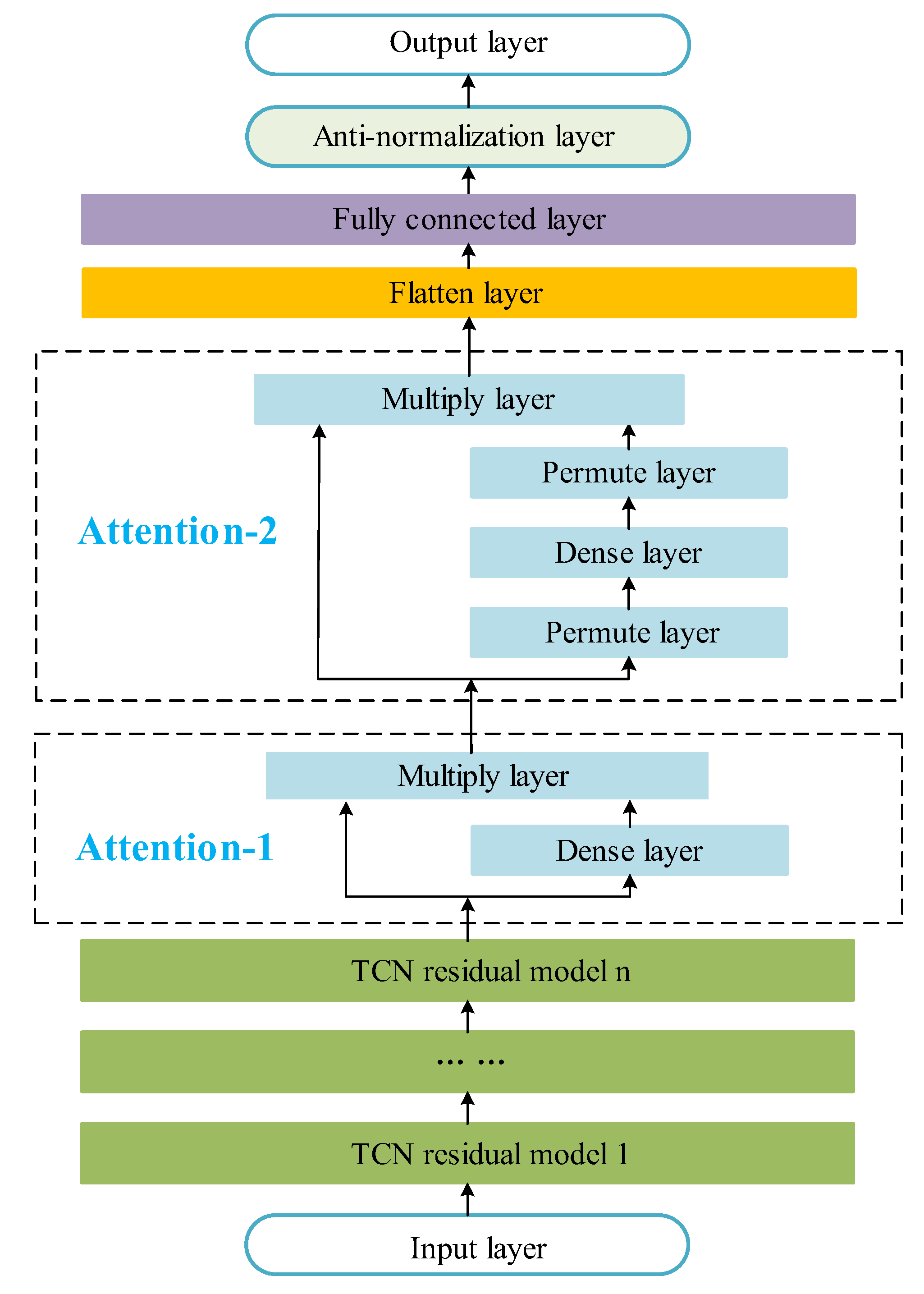
The essence of the attention mechanism is to filter out the important information from a large amount of information and focus on this information while ignoring the less important information [26,27,28]. The attention module gives a certain score by calculating the importance of different input features to the output result. For features with higher scores that are more critical, larger weight values will be assigned. By highlighting the influence of key features, thus improving the accuracy of the prediction model, the schematic diagram is shown in Figure 5.

As shown in Figure 5, $x_t\left(t\in \left[0,T\right]\right)$ represents the input sequence of the model, $h_t\left(t\in \left[0,T\right]\right)$ corresponds to the output of the hidden layer, $a_t\left(t\in \left[0,T\right]\right)$ is the attention weight of the current input to the historical input hidden layer state, and $F_t\left(t\in \left[0,T\right]\right)$ is the output value of the attention layer. The output of the attention layer is calculated as follows:

$$P_t=u \tan \mathrm{h}\left(w_t \ast h_t^{\mathrm{T}}+b_t\right)$$

(11)

$$a_t=\mathrm{softmax}\left(P_t\right)=\frac{\exp \left(P_t\right)}{{{\displaystyle \sum }}_{t=0}^T\exp \left(P_t\right)}$$

(12)

$$F_{\mathrm{t}}={{\displaystyle \sum }}_{t=0}^T{a}_t{h}_t$$

(13)

where $P_t$ is the similarity between the hidden layer state and different states, u and $w_t$ are the weight coefficients, tanh is the hyperbolic tangent function, and $b_t$ is the bias coefficient.

3.3. TCDAN Model

The temporal convolution double-layer attention network (TCDAN) proposed in this paper introduces a two-layer attention mechanism based on the TCN residual module, as shown in Figure 6. First, the input time-series is preliminarized through multiple TCN residual modules, and the convolution operation is used to capture the high and low-dimensional hidden features of the context sequence in the input data. The output of the TCN residual module maintains the same temporal dimension as the input data, and the feature dimension is increased by multiple convolution kernels. According to the input and output of the TCN residual module, Attention-1 mainly mines the correlation between the features corresponding to different input variables and the predictor variables. The Dense layer with SoftMax activation function is used to calculate the weight of each input, and the Multiply layer outputs the input and the corresponding assigned weight. Then, the influence of key features on the prediction results is highlighted. Compared to Attention-1, Attention-2 adds a Permute layer to adjust the dimensions of the input and output in the hidden layer. Therefore, the Dense layer in Attention-2 is applied to the time dimension to mine the influence of different time step data on the prediction results, and adjust the corresponding weights according to the contribution. After the Attention layer, the Flatten layer is used to flatten the multi-dimensional output in the Attention-2 layer. Finally, the prediction results were output by the fully connected layer and the predicted value was output after the anti-normalization layer processing.

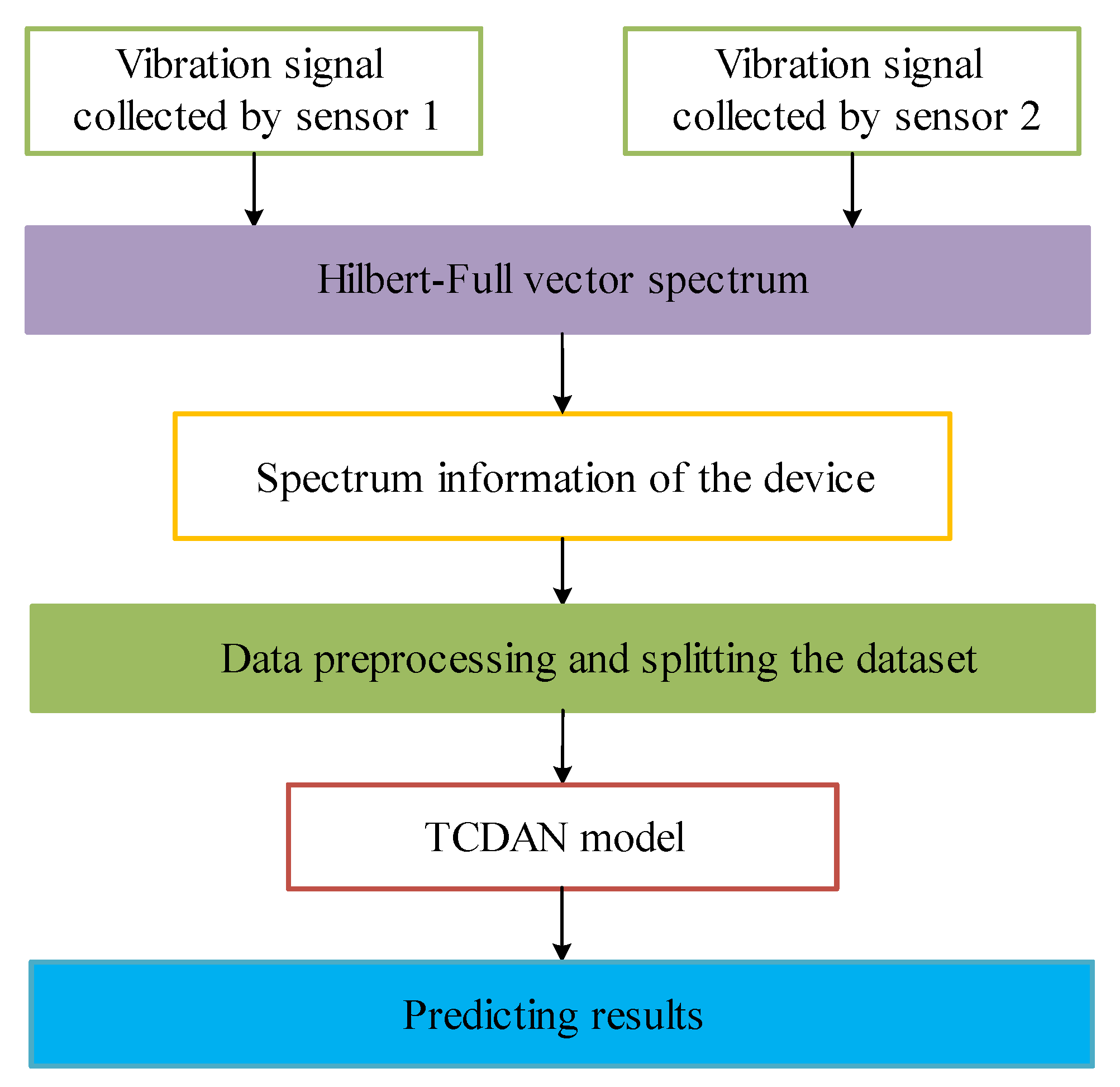
3.4. Process of Prediction

The fault-prediction process is shown in Figure 7, which is mainly divided into four steps, and the specific process is shown as follows:

Step 1: The vibration data of the dual channels of the device is processed based on the Hilbert–full-vector spectrum, and the amplitudes corresponding to different characteristic frequencies of the device are obtained.

Step 2: The amplitude data corresponding to each characteristic frequency obtained in Step 1 are normalized, and then divided into a training set and a test set according to the lag window size.

Step 3: Input the training set data processed in Step 2 into the TCDAN model, adjust the different parameters of the model for training and testing, and save the best prediction model according to the evaluation index of the test results.

Step 4: Make a prediction using the best-saved prediction model and output the prediction results.

In this paper, the mean absolute error (MAE), root mean squared error (root mean squared error, RMSE), and mean absolute percentage error (MAPE) was used to analyze the prediction results of each variable, and the calculation of each evaluation index was as follows:

$$\mathrm{MAE}=\frac{1}{n}{{\displaystyle \sum }}_{i=1}^n\left|{\widehat{y}}_i-y_i\right|$$

(14)

$$\mathrm{RMSE}=\sqrt{\frac{1}{n}{{\displaystyle \sum }}_{i=1}^n{\left({\widehat{y}}_i-y_i\right)}^2}$$

(15)

$$\mathrm{MAPE}=\frac{100\%}{n}{{\displaystyle \sum }}_{i=1}^n\left|\frac{{\widehat{y}}_i-y_i}{y_i}\right|$$

(16)

where n is the total number of samples, $y_i$ is the actual value and ${\widehat{y}}_i$ is the predicted value. MAE and RMSE represent the stability of the model—the smaller the value, the more stable the model. The MAPE is used to indicate the accuracy of the model; the closer the MAPE to 0, the more accurate the model.

4. Experiment Verification

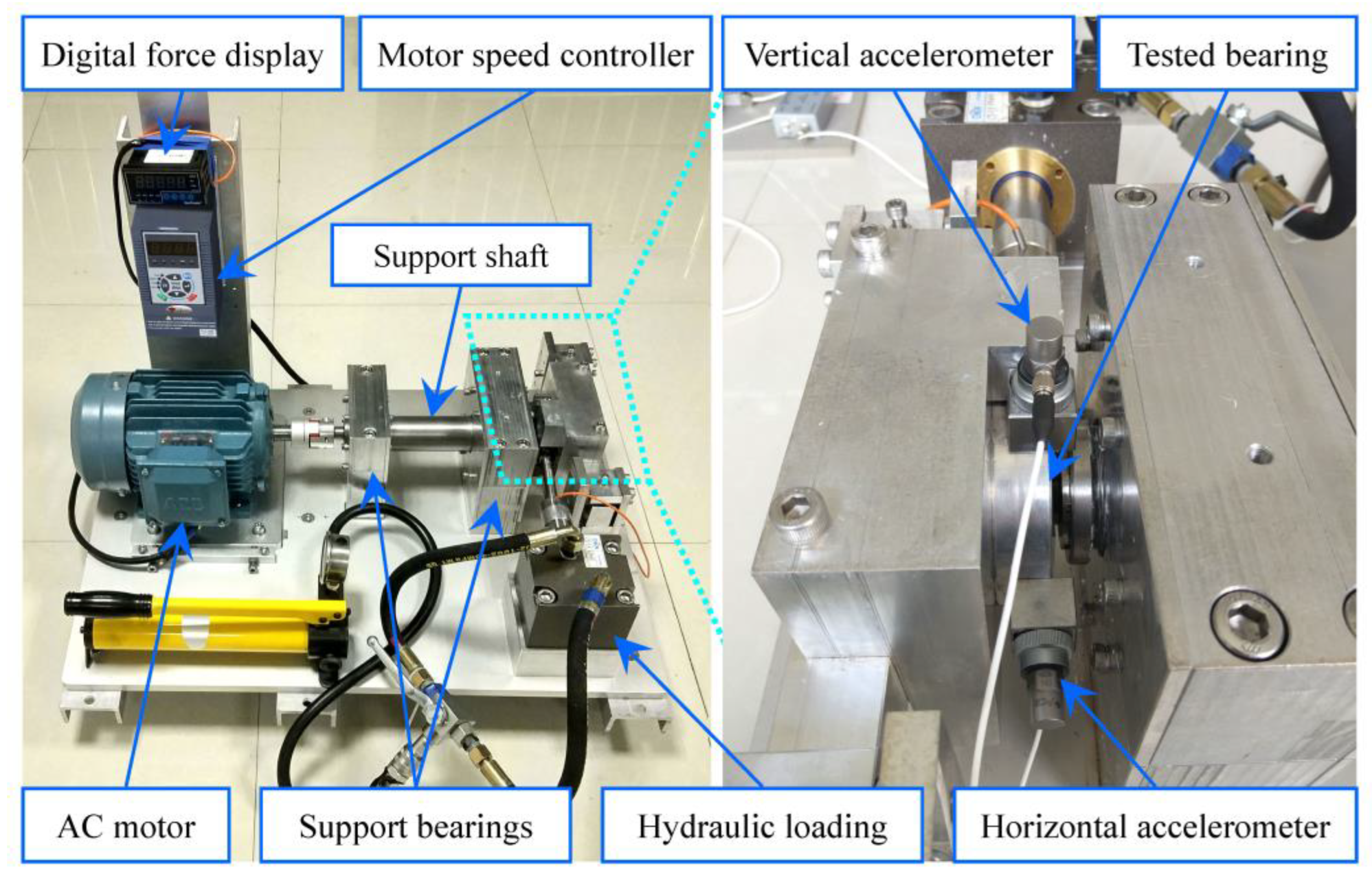
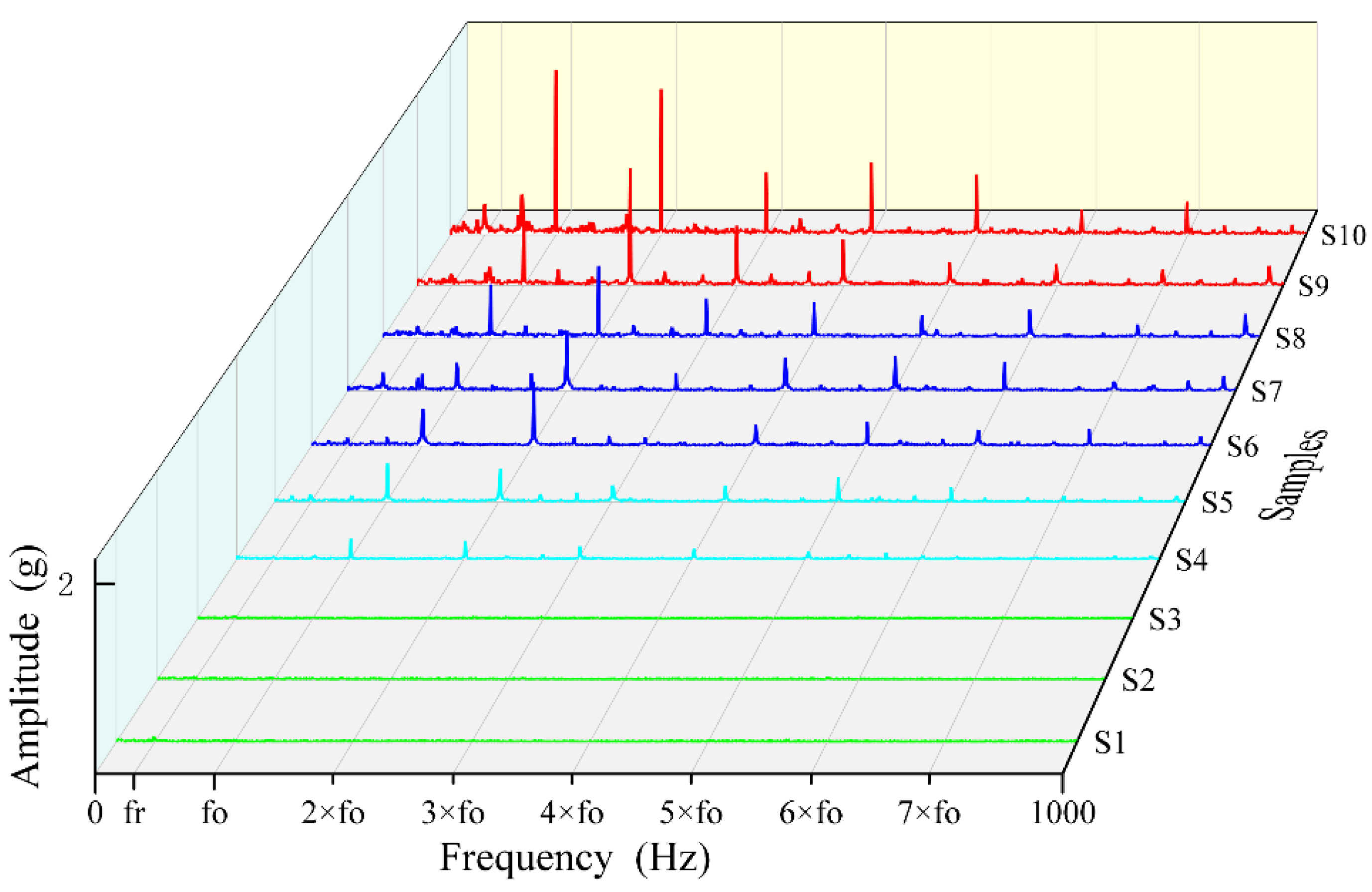
4.1. Introduction of Experimental Data

To verify the effectiveness of the proposed method, XJTU-SY bearing datasets that contain complete run-to-failure data of rolling element bearings were used, and the experimental platform is shown in Figure 8 [35]. The rotating shaft of the test bed is driven by an AC motor, and the supporting bearing model is the LDK UER204 rolling bearing, and the relevant specific parameters are shown in

Table 1. Parameters of Bearing 2_1 and Bearing 3_1.

Parameter	Value	Parameter	Value
Diameter of inner raceway/mm	29.30	Diameter of bearing rolling element/mm	7.92
Diameter of outer raceway/mm	39.80	The number of bearing rolling element	8
The pitch diameter of the bearing/mm	34.55	contact angle/°	0

. To obtain the life-cycle vibration signal of the bearing, two PCB 352C33 unidirectional acceleration sensors are fixed on the horizontal and vertical directions of the test bearing by magnetic seats, respectively. In the test, the sampling frequency was set as 25.6 kHz, the sampling interval was 1 min, and the duration of each sampling was 1.28 s. In this paper, Bearing 3_1 with the final outer-ring fault and Bearing 2_1 with the final inner-ring fault are taken as the experimental objects. For Bearing 3_1, its full life cycle is 42 h 18 min, the total number of samples is 2538, the operating speed is 2400 r/min, and the applied radial force is 10 kN. For Bearing 2_1, its full life cycle is 8 h 11 min, the total number of samples is 491, the operating speed is 2250 r/min, and the applied radial force is 11 kN.

The different characteristic frequencies of the bearing are calculated as follows:

Bearing rotation frequency $f_r$:

$$f_r=\frac{n}{60}$$

(17)

The fault characteristic frequency of the bearing outer ring $f_o$:

$$f_o=0.5z{f}_r\left(1-\frac{d}{D}\cos \alpha \right)$$

(18)

Fault characteristic frequency of bearing inner ring $f_i$:

$$f_i=0.5z{f}_r\left(1+\frac{d}{D}\cos \alpha \right)$$

(19)

The fault characteristic frequency of the bearing rolling element $f_R$:

$$f_R=\frac{D}{d}{f}_r\left[1-{\left(\frac{d}{D}\right)}^2{\cos }^2\alpha \right]$$

(20)

Fault characteristic frequency of bearing cage $f_c$:

$$f_c=0.5f_r\left(1-\frac{d}{D}\cos \alpha \right)$$

(21)

where $n$ is the rotation speed of the bearing, $d$ represents the diameter of the bearing rolling element, $D$ represents the pitch diameter of the bearing, $\mathsf{\alpha }$ represents the contact angle of the bearing, and z represents the number of bearing balls.

Combining Table 1 and Equations (17)–(21), it can be obtained that the rotation frequency $f_r$ of Bearing 3_1 is 40 Hz, the fault characteristic frequency of the outer ring $f_o$ is 123.32 Hz, the fault characteristic frequency of the inner ring $f_i$ is 196.68 Hz, and the fault characteristic frequency of the rolling element $f_R$ is 165.33 Hz. The fault characteristic frequency of the cage $f_c$ is 15.42 Hz.

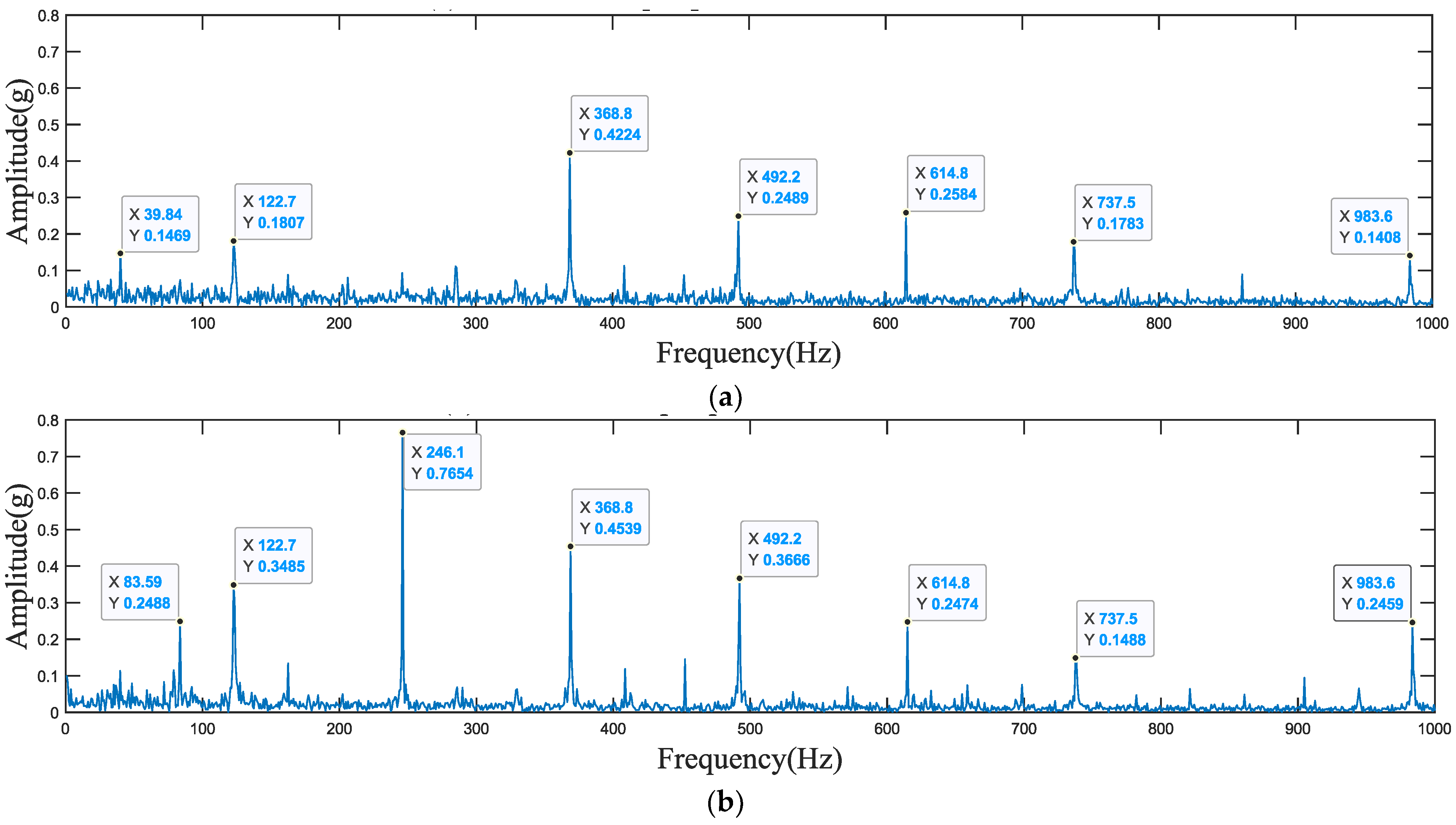
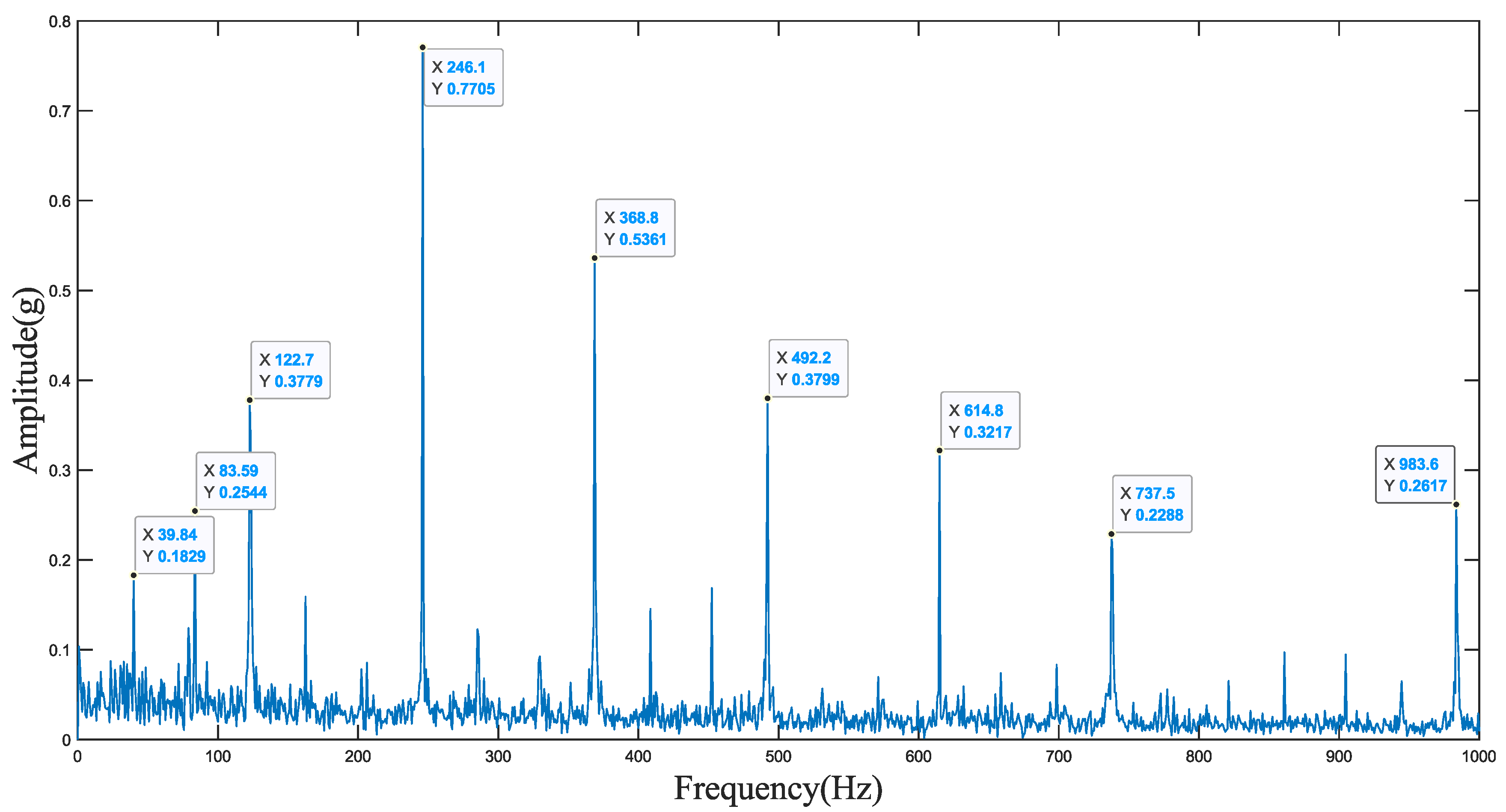
4.2. Application of Hilbert–Full-Vector Spectrum

Taking the data collected at 2510 min of Bearing 3_1 as an example, the vibration data collected in the horizontal and vertical directions were processed using the ordinary Hilbert-envelope spectrum [36,37] and Hilbert–full-vector spectrum technology, respectively, and the processing results are shown in Figure 9 and Figure 10.

As shown in Figure 9, the Hilbert-envelope spectrum in both directions has a certain prominent reflection at the outer-ring fault frequency of Bearing 3_1, which is consistent with the actual situation of bearing outer-ring fault, but the prominent characteristic frequency of the two is not completely consistent as a whole. According to Figure 9a, it can be seen that the horizontal Hilbert-envelope spectrum does not prominently reflect the 2 times frequency of the rotation frequency of Bearing 3_1 and the 2 times frequency of the outer-ring fault frequency. According to Figure 9b, it can be seen that the vertical Hilbert-envelope spectrum does not prominently reflect the 1 times frequency of the rotation frequency of Bearing 3_1. The Hilbert-envelope spectrum in either direction does not fully reflect the state information of Bearing 3_1.

As shown in Figure 10, the Hilbert–full-vector spectrum is prominently reflected in the rotation frequency, outer-ring fault frequency, and the corresponding frequency doubling of Bearing 3_1, and the outer-ring characteristic frequency and the corresponding frequency doubling are even more prominent, which reflects the outer-ring fault information of Bearing 3_1. Compared with the traditional Hilbert-envelope spectrum, the Hilbert–full-vector spectrum contains more comprehensive information about Bearing 3_1 by fusing the vibration data in two directions, and can better reflect the running state of Bearing 3_1.

The samples of the Bearing 3_1 health state, initial fault stage, middle fault stage, and late fault stage are, respectively, selected and processed based on the Hilbert–full-vector spectrum technique, as shown in Figure 11. The corresponding amplitudes of the rotation frequency, the outer-ring fault frequency, and the outer-ring fault frequency doubling of the bearing change obviously in different operating stages of Bearing 3_1. This change proves the effectiveness of using the corresponding amplitudes of different characteristic frequencies as equipment fault-prediction features.

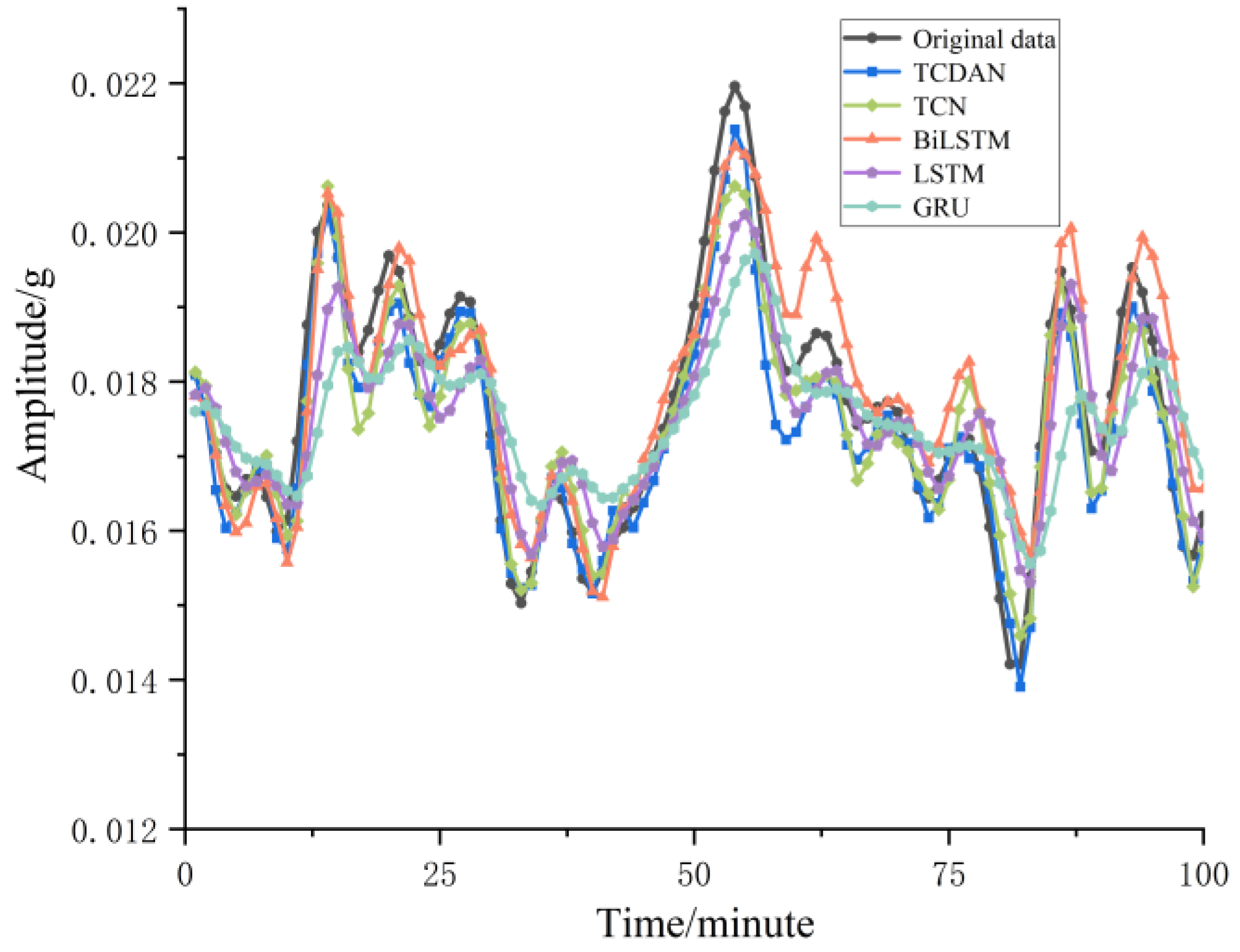
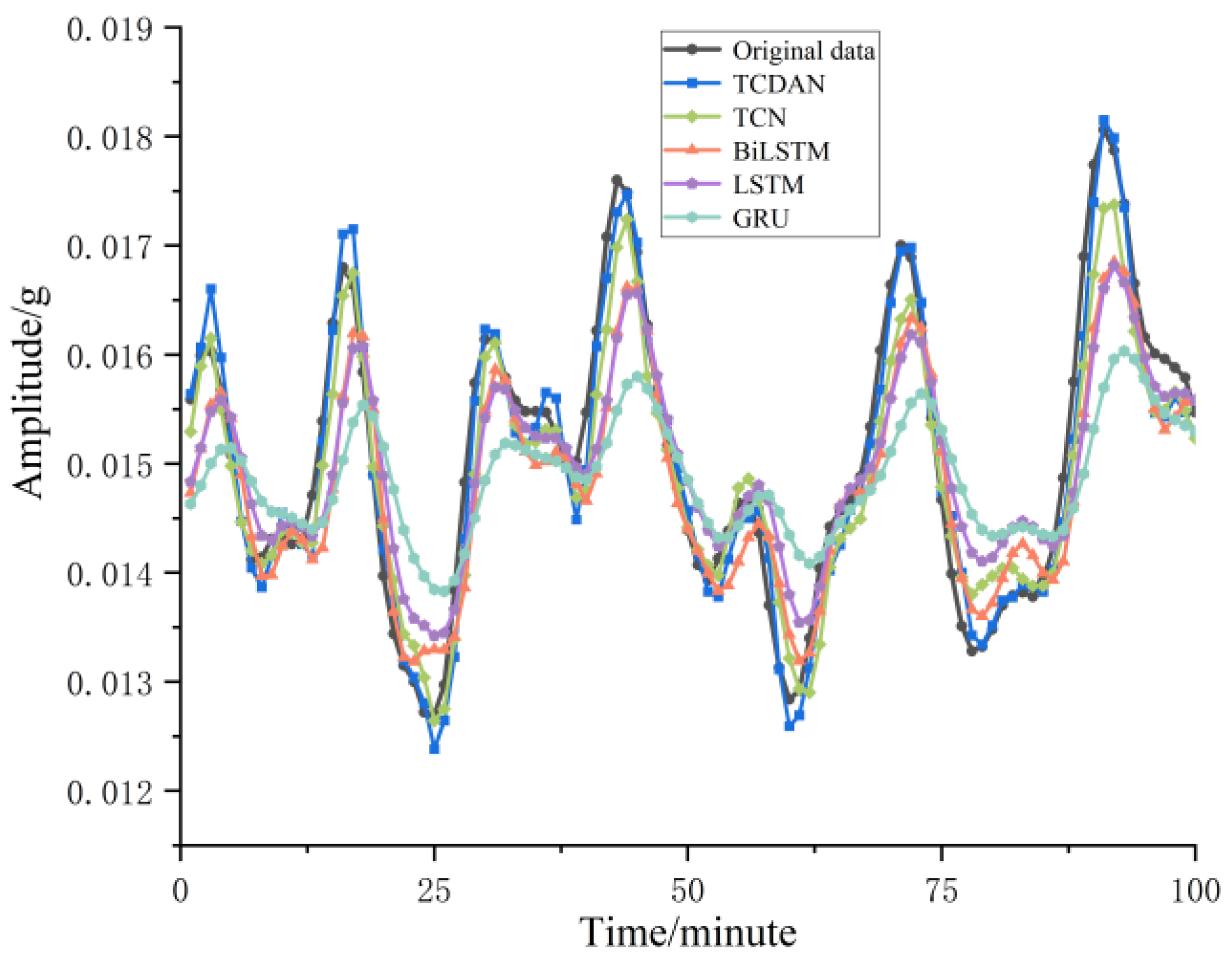
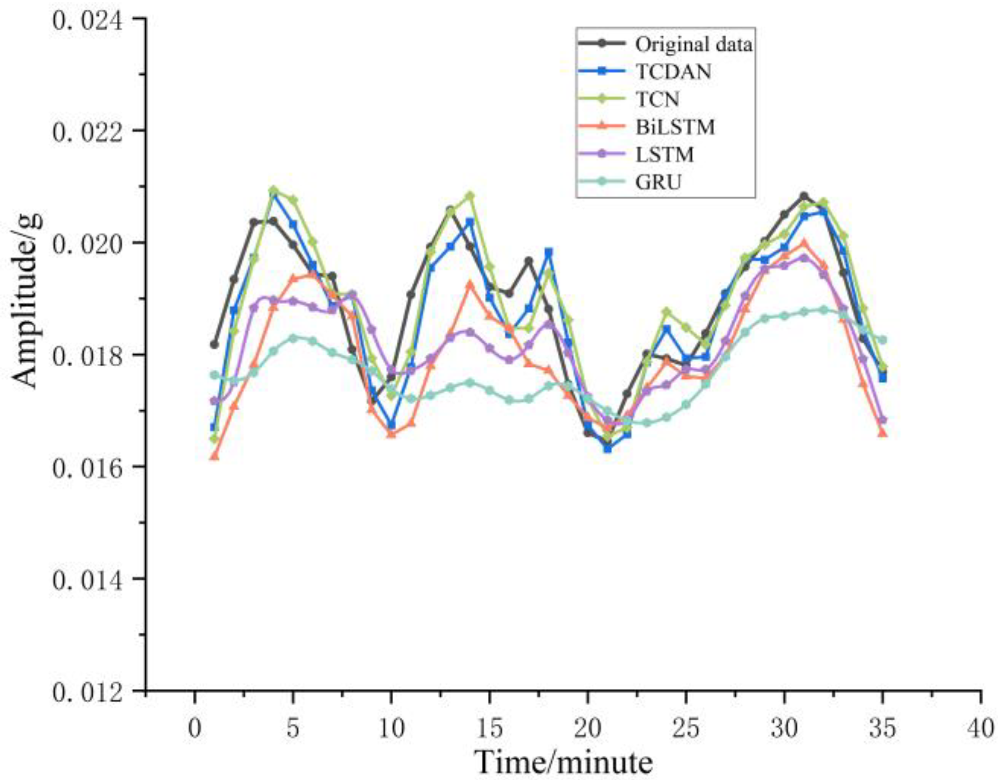
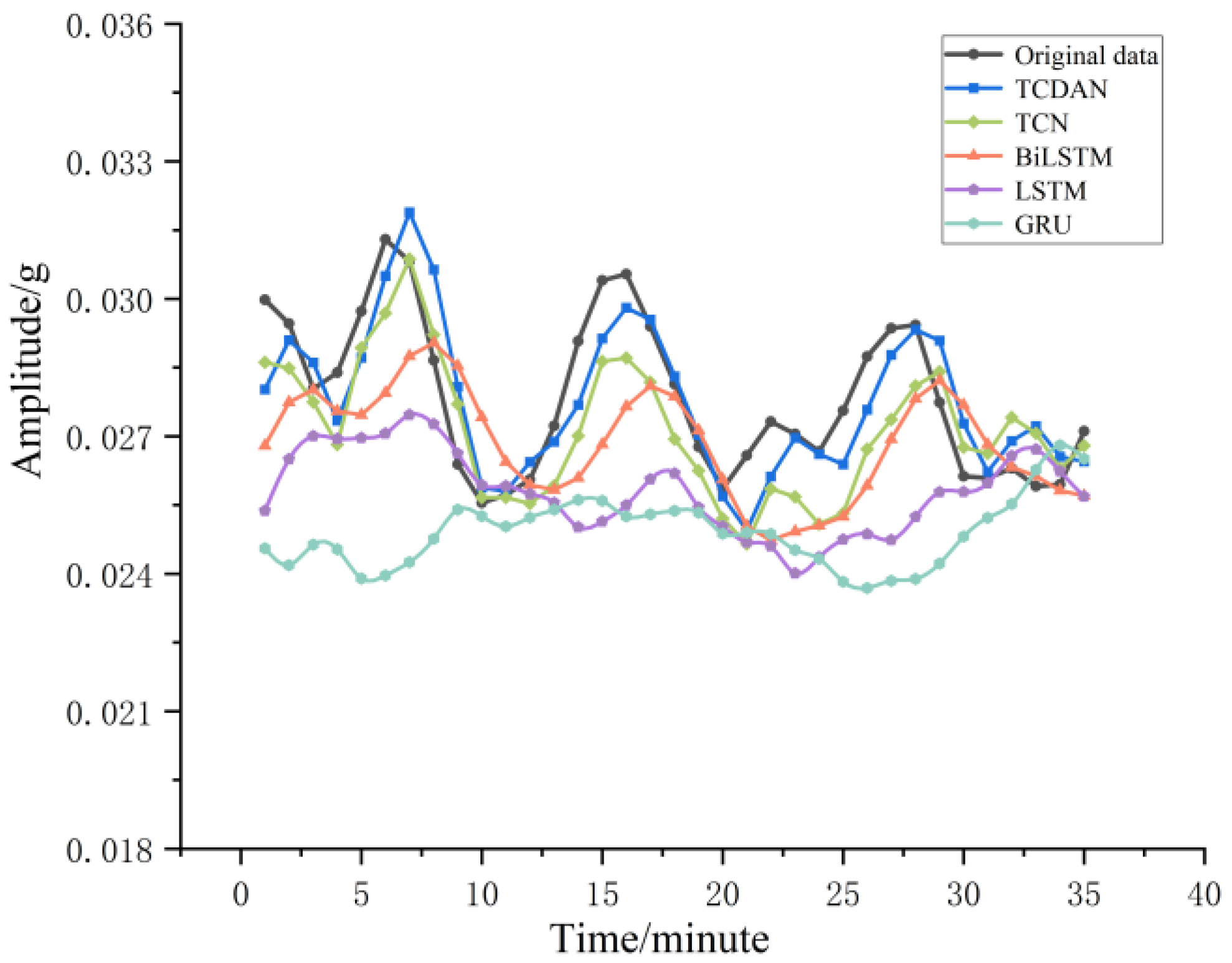
4.3. Performance Comparison of Prediction Models

First, the amplitudes corresponding to different characteristic frequencies in the life cycle of Bearing 3_1 are extracted based on the Hilbert–full-vector spectrum. According to the failure mechanism of the bearing [38], the amplitudes corresponding to the first and second times of the five characteristic frequencies of the bearing, which are the rotation frequency, the outer-ring fault frequency, the rolling element fault frequency, the cage fault frequency, and the inner-ring fault frequency, are taken as the input of the model, and the output variable is the amplitude corresponding to the characteristic frequency of concern after 1 min.

To illustrate the effectiveness of the prediction method proposed in this paper, the data of the past 2000 min (containing 2000 samples) is selected as the training set, and the data of the next 100 min (containing 100 samples) is selected as the test set. Based on the same dataset, the TCDAN proposed in this paper is compared with the TCN, GRU, and LSTM models.

The computer processor used in this experiment is Intel Core i5-4200H, and the graphics card is an NVIDIA GTX950M standalone graphics card with 8 GB memory. The model is based on Python language. Both the TCDAN and TCN models use two residual modules, the size of the convolution kernel is 3, the number of convolution kernels is 64, and the time step is 8; The LSTM and GRU models have eight hidden layers and 128 neurons. The input dimension of each model is 10, and the output dimension is 1. All models are developed based on the TensorFlow deep-learning framework and use the GPU to train the models. To speed up the convergence of the model, each variable is input into each model after normalization. Taking the prediction of the corresponding amplitude of the outer-ring fault frequency of Bearing 3_1 as an example, the prediction results of the corresponding amplitude of 1 and 2 times the outer-ring fault frequency of different models are shown in Figure 12 and Figure 13, respectively.

Through the comparison of the prediction effects of different models in Figure 12 and Figure 13, it can be seen that the proposed TCDAN has higher prediction accuracy compared with the TCN without attention mechanism. At the same time, the prediction performance of TCDAN is also significantly better than that of the current mainstream prediction models such as BiLSTM, LSTM, and GRU. Combined with the evaluation indexes of the prediction results of each model in

Table 2. Evaluation metrics of different prediction models for Bearing 3_1.

Models	MAE		RMSE		MAPE(%)
	1 × fo	2 × fo	1 × fo	2 × fo	1 × fo	2 × fo
TCDAN	0.0240	0.0317	0.0297	0.0382	6.04	6.34
TCN	0.0490	0.0465	0.0608	0.0579	10.91	9.28
BiLSTM	0.0550	0.0682	0.0694	0.0881	15.63	12.79
LSTM	0.0798	0.0773	0.0921	0.0991	26.58	27.14
GRU	0.0966	0.1023	0.1221	0.1278	32.37	34.71

, it can be seen that the MAE, RMSE, and MAPE prediction indexes of the amplitude corresponding to 1 times the outer-ring fault frequency predicted by TCDAN are reduced to 0.0240, 0.0297, and 6.04%, respectively. The MAE, RMSE, and MAPE prediction indexes of the amplitude corresponding to 2 times the outer-ring fault frequency are reduced to 0.0317, 0.0382, and 6.34%, respectively. Compared with TCN, GRU, BiLSTM, and LSTM models, TCDAN has greatly improved the prediction performance.

To verify the generalization ability of the TCDAN model, the data of Bearing 2_1 in the XJTU-SY dataset were used for experiments based on the same experimental process. Considering the smaller sample size of the Bearing 2_1 data, the data of 35 min (containing 35 samples) was selected as the test set, and different models trained based on the Bearing 3_1 data were used for testing. Taking the prediction of the corresponding amplitude of the inner-ring fault frequency of Bearing 2_1 as an example, the prediction results of the corresponding amplitude of the inner-ring fault frequency of 1 and 2 times by different models are shown in Figure 14 and Figure 15, respectively.

Through the comparison of the prediction effects of different models in Figure 14 and Figure 15, the prediction performance of TCDAN is significantly better than that of TCN, BiLSTM, LSTM, and GRU. Combined with the evaluation indexes of the prediction results of each model in

Table 3. Evaluation metrics of different prediction models for Bearing 2_1.

Models	MAE		RMSE		MAPE(%)
	1 × fi	2 × fi	1 × fi	2 × fi	1 × fi	2 × fi
TCDAN	0.0471	0.0496	0.0583	0.0609	9.69	6.27
TCN	0.0534	0.0735	0.0653	0.0836	11.39	9.09
BiLSTM	0.0921	0.0958	0.1151	0.1168	17.51	11.75
LSTM	0.0926	0.1386	0.1079	0.1704	22.79	16.55
GRU	0.1300	0.1910	0.1522	0.2292	27.29	22.75

, it can be seen that the MAE, RMSE, and MAPE prediction indexes of the amplitude corresponding to 1 times the inner-ring fault frequency predicted by TCDAN are reduced to 0.0471, 0.0583, and 9.69%, respectively. The MAE, RMSE, and MAPE prediction indexes of the amplitude corresponding to 2 times the inner-ring fault frequency are reduced to 0.0497, 0.0609, and 6.27%, respectively. Compared with TCN, GRU, BiLSTM, and LSTM models, TCDAN still has the best prediction performance, which verifies the good generalization ability of the TCDAN model.

5. Conclusions

In this paper, the Hilbert–full-vector spectrum is used to extract the spectrum information of equipment. Compared with the traditional Hilbert-envelope spectrum, the Hilbert–full-vector spectrum fuses the vibration data of the dual channels of the equipment, which can more comprehensively reflect the actual operational state of the equipment as a fault-prediction feature. In addition, combined with the two-layer attention mechanism, a temporal convolutional network is used to predict the amplitude corresponding to different characteristic frequencies of the device. Compared with TCN, GRU, BiLSTM, and LSTM models, the TCDAN model proposed in this paper can effectively extract the correlation between different variables in historical data, different time step data, and predictor variables, to adjust the corresponding weight size, and has higher prediction accuracy.

Through the prediction of the amplitude corresponding to the characteristic frequency of the equipment, the fault trend of the equipment can be intuitively seen, and the specific part of the equipment fault can be judged according to the characteristic frequency, which provides a more effective decision-making basis for the predictive maintenance of the equipment. In the future, the correlation between the amplitude corresponding to different characteristic frequencies and the fault degree will be studied, so that the alarm threshold corresponding to the amplitude of different characteristic frequencies can be set for better application in actual production.

References

1. Kordestani, M.; Rezamand, M.; Orchard, M.E.; Carriveau, R.; Ting, D.S.-K.; Rueda, L.; Saif, M. New Condition-Based Monitoring and Fusion Approaches With a Bounded Uncertainty for Bearing Lifetime Prediction. IEEE Sens. J. 2022, 22, 9078–9086. [Google Scholar] [CrossRef]
2. Igba, J.; Alemzadeh, K.; Durugbo, C.; Eiriksson, E.T. Analysing RMS and Peak Values of Vibration Signals for Condition Monitoring of Wind Turbine Gearboxes. Renew. Energy 2016, 91, 90–106. [Google Scholar] [CrossRef] [Green Version]
3. Brotherton, T.; Grabill, P.; Wroblewski, D.; Friend, R.; Sotomayer, B.; Berry, J. A Testbed for Data Fusion for Engine Diagnostics and Prognostics. In Proceedings of the 2002 IEEE Aerospace Conference, Big Sky, MT, USA, 9–16 March 2002; Volume 6, p. 6. [Google Scholar]
4. Luo, J.; Namburu, M.; Pattipati, K.; Qiao, L.; Kawamoto, M.; Chigusa, S. Model-Based Prognostic Techniques [Maintenance Applications]. In Proceedings of the Autotestcon 2003, IEEE Systems Readiness Technology Conference, Anaheim, CA, USA, 22–25 September 2003; pp. 330–340. [Google Scholar]
5. Xu, J.; Xu, L. Health Management Based on Fusion Prognostics for Avionics Systems. J. Syst. Eng. Electron. 2011, 22, 428–436. [Google Scholar] [CrossRef]
6. Practical Options for Selecting Data-Driven or Physics-Based Prognostics Algorithms with Reviews. Reliab. Eng. Syst. Saf. 2015, 133, 223–236. [CrossRef]
7. Coppe, A.; Pais, M.J.; Haftka, R.T.; Kim, N.H. Using a Simple Crack Growth Model in Predicting Remaining Useful Life. J. Aircr. 2012, 49, 1965–1973. [Google Scholar] [CrossRef]
8. Xu, H.; Ma, R.; Yan, L.; Ma, Z. Two-Stage Prediction of Machinery Fault Trend Based on Deep Learning for Time Series Analysis. Digit. Signal Process. 2021, 117, 103150. [Google Scholar] [CrossRef]
9. Dang, P.; Zhang, H.; Yun, X.; Ren, H. Fault Prediction of Rolling Bearing Based on ARMA Model. In Proceedings of the 2017 International Conference on Computer Systems, Electronics and Control (ICCSEC), Dalian, China, 25–27 December 2017; pp. 725–728. [Google Scholar]
10. Xue, P.; Xu, Y.; Liu, N. The Study of Optimized Grey Model Using for Transformer Fault Prediction. In Proceedings of the 4th International Symposium on Power Electronics and Control Engineering (ISPECE 2021), Nanchang, China, 29 November 2021; Volume 12080, pp. 835–844. [Google Scholar]
11. Soualhi, A.; Medjaher, K.; Zerhouni, N. Bearing Health Monitoring Based on Hilbert–Huang Transform, Support Vector Machine, and Regression. IEEE Trans. Instrum. Meas. 2015, 64, 52–62. [Google Scholar] [CrossRef] [Green Version]
12. Benkedjouh, T.; Medjaher, K.; Zerhouni, N.; Rechak, S. Health Assessment and Life Prediction of Cutting Tools Based on Support Vector Regression. J. Intell. Manuf. 2015, 26, 213–223. [Google Scholar] [CrossRef] [Green Version]
13. Azadeh, A.; Saberi, M.; Kazem, A.; Ebrahimipour, V.; Nourmohammadzadeh, A.; Saberi, Z. A Flexible Algorithm for Fault Diagnosis in a Centrifugal Pump with Corrupted Data and Noise Based on ANN and Support Vector Machine with Hyper-Parameters Optimization. Appl. Soft Comput. 2013, 13, 1478–1485. [Google Scholar] [CrossRef]
14. Guo, L.; Li, N.; Jia, F.; Lei, Y.; Lin, J. A Recurrent Neural Network Based Health Indicator for Remaining Useful Life Prediction of Bearings. Neurocomputing 2017, 240, 98–109. [Google Scholar] [CrossRef]
15. Ling, J.; Liu, G.-J.; Li, J.-L.; Shen, X.-C.; You, D.-D. Fault Prediction Method for Nuclear Power Machinery Based on Bayesian PPCA Recurrent Neural Network Model. Nucl. Sci. Technol. 2020, 31, 75. [Google Scholar] [CrossRef]
16. Ma, M.; Mao, Z. Deep-Convolution-Based LSTM Network for Remaining Useful Life Prediction. IEEE Trans. Ind. Inform. 2021, 17, 1658–1667. [Google Scholar] [CrossRef]
17. Branco, N.W.; Cavalca, M.S.M.; Stefenon, S.F.; Leithardt, V.R.Q. Wavelet LSTM for Fault Forecasting in Electrical Power Grids. Sensors 2022, 22, 8323. [Google Scholar] [CrossRef]
18. Zheng, L.; Chen, J.; Chen, F.; Chen, B.; Xue, W.; Guo, P.; Li, J. Rotating Machinery Fault Prediction Method Based on Bi-LSTM and Attention Mechanism. In Proceedings of the 2019 IEEE International Conference on Energy Internet (ICEI), Nanjing, China, 27–31 May 2019; pp. 53–58. [Google Scholar]
19. Liang, T.; Meng, Z.; Xie, G.; Fan, S. Multi-Running State Health Assessment of Wind Turbines Drive System Based on BiLSTM and GMM. IEEE Access 2020, 8, 143042–143054. [Google Scholar] [CrossRef]
20. Ren, L.; Cheng, X.; Wang, X.; Cui, J.; Zhang, L. Multi-Scale Dense Gate Recurrent Unit Networks for Bearing Remaining Useful Life Prediction. Future Gener. Comput. Syst. 2019, 94, 601–609. [Google Scholar] [CrossRef]
21. Qin, Y.; Chen, D.; Xiang, S.; Zhu, C. Gated Dual Attention Unit Neural Networks for Remaining Useful Life Prediction of Rolling Bearings. IEEE Trans. Ind. Inform. 2021, 17, 6438–6447. [Google Scholar] [CrossRef]
22. Bai, S.; Kolter, J.Z.; Koltun, V. An Empirical Evaluation of Generic Convolutional and Recurrent Networks for Sequence Modeling. arXiv 2018, arXiv:1803.01271. [Google Scholar]
23. Chen, Q.; Liu, Y.-B.; Ge, M.-F.; Liu, J.; Wang, L. A Novel Bayesian-Optimization-Based Adversarial TCN for RUL Prediction of Bearings. IEEE Sens. J. 2022, 22, 20968–20977. [Google Scholar] [CrossRef]
24. Chen, Y.; Kang, Y.; Chen, Y.; Wang, Z. Probabilistic Forecasting with Temporal Convolutional Neural Network. Neurocomputing 2020, 399, 491–501. [Google Scholar] [CrossRef] [Green Version]
25. Lin, Y.; Koprinska, I.; Rana, M. Temporal Convolutional Attention Neural Networks for Time Series Forecasting. In Proceedings of the 2021 International Joint Conference on Neural Networks (IJCNN), Shenzhen, China, 18–22 July 2021; pp. 1–8. [Google Scholar]
26. Mnih, V.; Heess, N.; Graves, A.; Kavukcuoglu, K. Recurrent Models of Visual Attention. arXiv 2014, arXiv:1406.6247. [Google Scholar] [CrossRef]
27. Bahdanau, D.; Cho, K.; Bengio, Y. Neural Machine Translation by Jointly Learning to Align and Translate. In Proceedings of the International Conference on Learning Representations, Banff, AB, Canada, 14–16 April 2014. [Google Scholar]
28. Vaswani, A.; Shazeer, N.; Parmar, N.; Uszkoreit, J.; Jones, L.; Gomez, A.N.; Kaiser, Ł.; Polosukhin, I. Attention Is All You Need. In Proceedings of the 31st International Conference on Neural Information Processing Systems, Long Beach, CA, USA, 4 December 2017; pp. 6000–6010. [Google Scholar]
29. Huang, N.E.; Shen, Z.; Long, S.R.; Wu, M.C.; Shih, H.H.; Zheng, Q.; Yen, N.-C.; Tung, C.C.; Liu, H.H. The Empirical Mode Decomposition and the Hilbert Spectrum for Nonlinear and Non-Stationary Time Series Analysis. Proc. R. Soc. Lond. A 1998, 454, 903–995. [Google Scholar] [CrossRef]
30. Huang, N.E.; Shen, Z.; Long, S.R. A New View of Nonlinear Water Waves: The Hilbert Spectrum. Annu. Rev. Fluid Mech. 1999, 31, 417–457. [Google Scholar] [CrossRef] [Green Version]
31. Chen, L.; Han, J.; Lei, W.; Cui, Y.; Guan, Z. Full-Vector Signal Acquisition and Information Fusion for the Fault Prediction. Int. J. Rotating Mach. 2016, 2016, e5980802. [Google Scholar] [CrossRef] [Green Version]
32. Chen, L.; Han, J.; Lei, W.; Guan, Z.; Gao, Y. Prediction Model of Vibration Feature for Equipment Maintenance Based on Full Vector Spectrum. Shock. Vib. 2017, 2017, 6103947. [Google Scholar] [CrossRef] [Green Version]
33. He, K.; Zhang, X.; Ren, S.; Sun, J. Deep Residual Learning for Image Recognition. In Proceedings of the 2016 IEEE Conference on Computer Vision and Pattern Recognition (CVPR), Las Vegas, NV, USA, 27–30 June 2016; pp. 770–778. [Google Scholar]
34. Salimans, T.; Kingma, D.P. Weight Normalization: A Simple Reparameterization to Accelerate Training of Deep Neural Networks. In Proceedings of the 30th International Conference on Neural Information Processing Systems, Barcelona, Spain, 5–10 December 2016; pp. 901–909. [Google Scholar]
35. Wang, B.; Lei, Y.; Li, N.; Li, N. A Hybrid Prognostics Approach for Estimating Remaining Useful Life of Rolling Element Bearings. IEEE Trans. Reliab. 2020, 69, 401–412. [Google Scholar] [CrossRef]
36. Huang, Z.; Xie, Y. Fault Diagnosis of Roller Bearing with Inner and External Fault Based on Hilbert Transformation. J. Cent. South Univ. (Sci. Technol.) 2011, 42, 1992–1996. [Google Scholar]
37. Yang, L.; Chen, L. Fault Diagnosis Algorithm of Printing Machine Rolling Bearing Based on Hilbert Envelope Spectrum. In Proceedings of the 2022 International Conference on Computer Network, Electronic and Automation (ICCNEA), Xi’an, China, 23–25 September 2022; pp. 357–361. [Google Scholar]
38. ISO 13373-3:2015; Condition Monitoring and Diagnostics of Machines—Vibration Condition Monitoring—Part 3: Guidelines for Vibration Diagnosis. ISO: Geneve, Switzerland, 2015. Available online: https://www.iso.org/standard/40840.html (accessed on 3 February 2023).
Figure 1. Layout of sensors: (a) Being installed in the horizontal–vertical direction; (b) Being installed in the V-shaped direction.
Applsci 13 04655 g001
Figure 2. The processing flow of fault feature extraction: (a) The processing flow of the traditional Hilbert-envelope spectrum; (b)The processing flow of the Hilbert–full-vector spectrum.
Applsci 13 04655 g002
Figure 3. Structure of dilated causal convolutions.
Applsci 13 04655 g003
Figure 4. The structure of the TCN residual model.
Applsci 13 04655 g004
Figure 5. Schematic of the attention mechanism.
Applsci 13 04655 g005
Figure 6. Structure of TCDAN.
Applsci 13 04655 g006
Figure 7. The flowchart of fault prediction.
Applsci 13 04655 g007
Figure 8. Bearing testbed.
Applsci 13 04655 g008
Figure 9. Hilbert-envelope spectrum: (a) Hilbert-envelope spectrum of horizontal direction; (b) Hilbert-envelope spectrum of vertical direction.
Applsci 13 04655 g009
Figure 10. Hilbert-envelope full-vector spectrum.
Applsci 13 04655 g010
Figure 11. Spectral changes in Bearing 3_1 in different periods. In this figure, fr stands for the rotational frequency of Bearing 3_1, fo stands for the outer-ring fault frequency of Bearing 3_1, 2 × fo, 3 × fo… 7 × fo represents the doubling frequency of Bearing 3-1 outer-ring fault frequency; S1, S2, and S3 represent the spectrum of the Bearing 3_1 health state, S4 and S5 represent the spectrum at the initial stage of the fault, S6, S7 and S8 represent the spectrum at the middle stage of the fault, and S9 and S10 represent the spectrum at the late stage of the fault.
Applsci 13 04655 g011
Figure 12. Prediction comparison of the amplitude corresponding to 1 × fo.
Applsci 13 04655 g012
Figure 13. Prediction comparison of the amplitude corresponding to 2 × fo.
Applsci 13 04655 g013
Figure 14. Prediction comparison of the amplitude corresponding to 1 × fi.
Applsci 13 04655 g014
Figure 15. Prediction comparison of the amplitude corresponding to 2 × fi.
Applsci 13 04655 g015