Article

Motor On-Line Fault Diagnosis Method Research Based on 1D-CNN and Multi-Sensor Information

School of Engineering Machinery, Chang’an University, Xi’an 710064, China
*
Author to whom correspondence should be addressed.
Appl. Sci. 2023, 13(7), 4192; https://doi.org/10.3390/app13074192
Submission received: 28 February 2023 / Revised: 23 March 2023 / Accepted: 23 March 2023 / Published: 25 March 2023

Abstract

:
The motor is the primary impetus source of most mechanical equipment, and its failure will cause substantial economic losses and safety problems. Therefore, it is necessary to study online fault diagnosis techniques for motors, given the problems caused by shallow learning models or single-sensor fault analysis in previous motor fault diagnosis techniques, such as blurred fault features, inaccurate identification, and time and manpower consumption. In this paper, we proposed a model for motor fault diagnosis based on deep learning and multi-sensor information fusion. Firstly, a correlation adaptive weighting method is proposed in this paper, and it is used to integrate the collected multi-source homogeneous sensor information into multi-source heterogeneous sensor information through the data layer fusion. Secondly, the 1D-CNN is used to carry out feature extraction, feature layer fusion, and fault classification of multi-source heterogeneous information of the motor. Finally, the data of seven states (one healthy and six faulty) of the motor are collected by the motor drive test bench to realize the model’s training, testing, and verification. The experimental results show that the fault diagnosis accuracy of the model is 99.3%. Thus, this method has important practical implications for improving the accuracy of motor fault diagnosis further.

1. Introduction

Monitoring the running state and accurately diagnosing faults of the motor has great significance for the safe operation of the transmission system [1]. The types of motor faults are numerous and complex, and they can be divided into stator faults, rotor faults, and bearing faults according to the location of the faults [2]. Due to the complex nonlinear mapping relationship between these fault types and fault signals, fault diagnosis is rather complicated [3].
Among traditional methods for motor fault diagnosis, they are generally based on single-sensor signal analysis or intelligent learning. In this literature study [4], to increase effective information on the fault features to diagnose the motor, wavelet transform is used to extract the features of the motor stator current, and the adaptive filter eliminated the fundamental component in the stator current. In this literature study [5], a research method is proposed to convert three stator currents of a motor into images with three different resolutions. In this method, the obtained image is used as the input of the multi-layer artificial neural network, and the network is trained and optimized by many samples. Finally, the optimized model with higher diagnostic accuracy is obtained. In this literature study [6], a deep belief network (DBN) is proposed. By training the network using the real-time acquired image-based vibration signals as input, tool fault diagnosis and identification of tool fault changes during milling are achieved. In this literature study [7], the deep learning method of the convolutional neural network (CNN) is adopted to extract multi-scale features from the original vibration signals, using the adaptive convolution operation to reduce each feature map to the same size for fusion. The fused fault features were finally classified using the Softmax function. In this literature study [8], different convolutional neural network architectures (such as AlexNet, ResNet-50, LeNet-5, and VGG-16) are designed and adapted to monitor the health of milling cutters, respectively. In addition, this article analyzed and discussed the classification accuracy, recall, advantages, and disadvantages of convolutional neural networks with different architectures. It has important implications for the design of our network architecture. As seen from the above research methods, which play an important guiding role in this paper, the research on fault diagnosis methods is deepening with technology development. However, all the above studies are based on a single sensor for fault diagnosis. Although a single sensor has good stability and data complexity, it has a low fault tolerance rate and limited fault information.
To improve the diagnostic accuracy rate, Multi-sensor Data Fusion (MDF) technology has become an important research direction of fault diagnosis. In this literature study [9], a multi-channel one-dimensional convolutional neural network is proposed. It used two vibration sensors in different directions to detect and diagnose six types of motor faults. Compared to a single vibrational signal, its diagnostic accuracy is improved. In this literature study [10], a spatiotemporal multi-correlation fusion method for multi-source vibration fault signals is proposed. This method utilized multiple interrelationships of spatial positions to explore the correlation between vibration sensors at different places, effectively improving the connection between sensor data. In this literature study [11], a fault diagnosis method is proposed, which is based on the feature layer fusion of vibration and acoustic signals of 1D-CNN. In this method, two types of dissimilarity information are taken as the input of 1D-CNN simultaneously, and the features are extracted, fused, and output. The cited literature study [12] is a further optimization of the previous study [11]. Firstly, the multi-sensor information is divided into homologous and heterogeneous categories. Secondly, the variance contribution rate method transformed homologous information into heterogeneous information through the data layer fusion. Secondly, The adaptive convolutional neural network (ADCNN) fused the heterogeneous information in the feature layers. Finally, the output fault features are classified by the Softmax function.
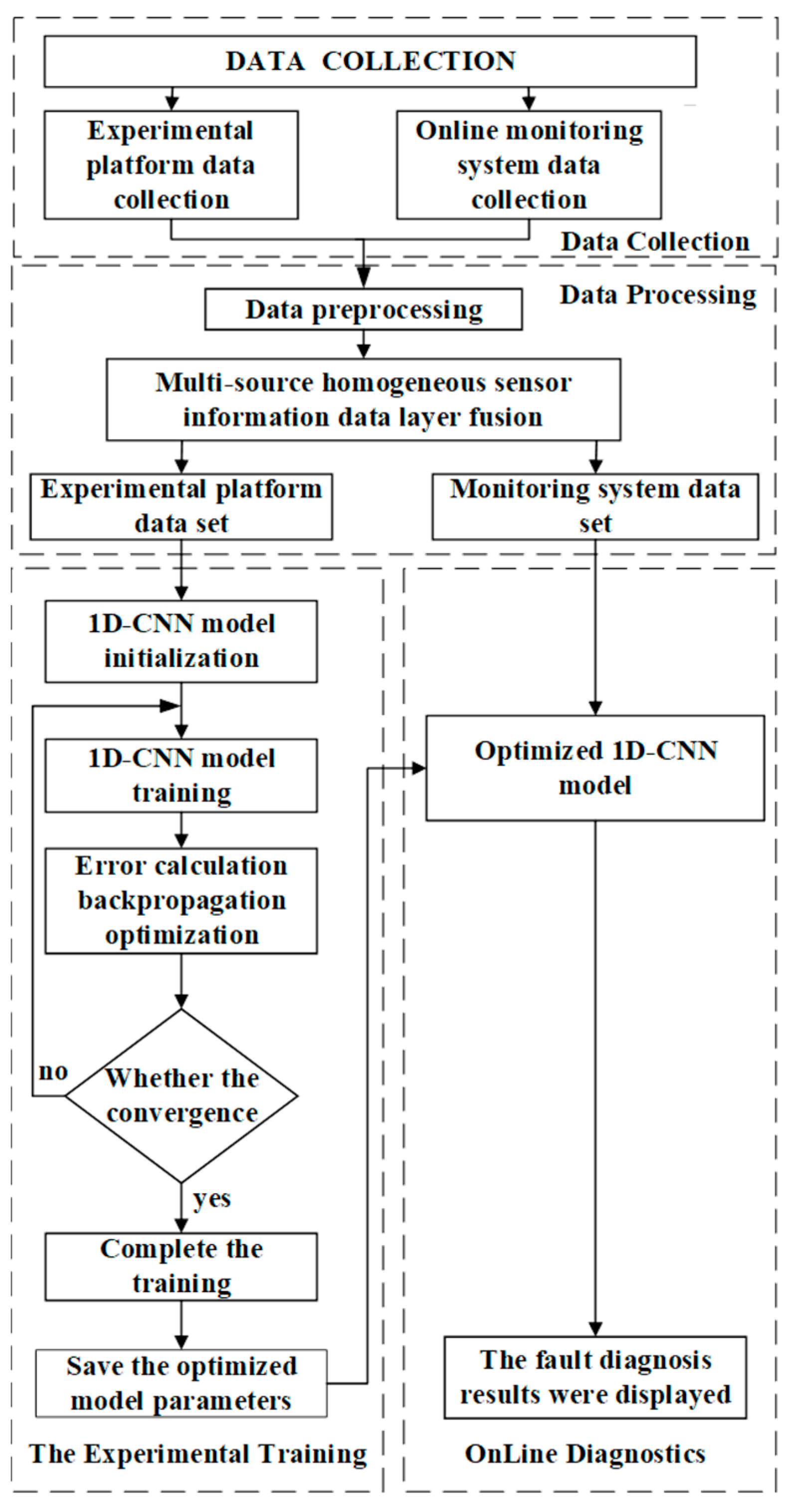
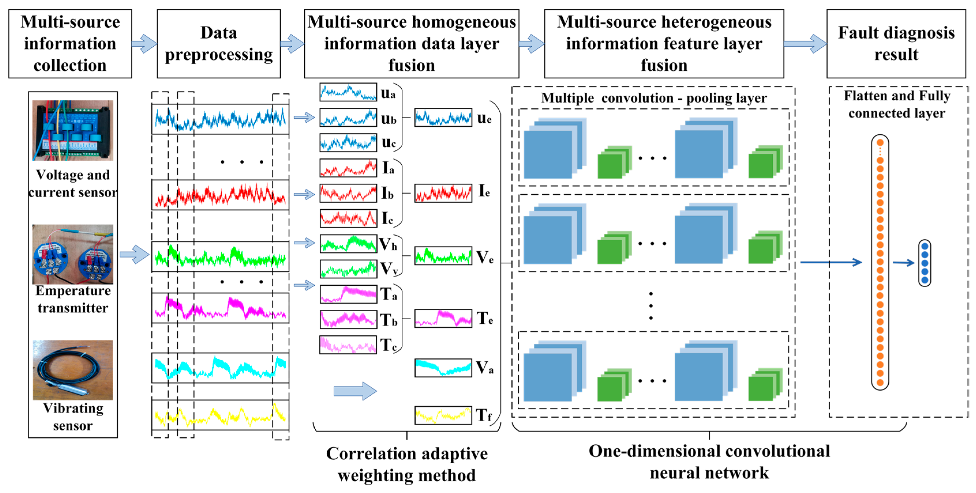
From the above literature study, there are many kinds of signals to be detected in the motor fault diagnosis, and the single feature fusion or variance contribution rate cannot fully use the correlation and complementarity among multi-source sensor information, which have certain data missing. For these problems, Firstly, the correlation adaptive weighting method is used to fuse the homologous information in the data layer in this paper. Secondly, 1D-CNN is used to fuse the heterogeneous information in the feature layers. Then the motor fault diagnosis model based on 1D-CNN and multi-sensor information fusion was established. Finally, the accurate diagnosis of motor faults is realized through the training of a large number of experimental data.

2. Motor Multi-Source Information Fusion Processing

2.1. Composition of Multi-Source Sensor Information of The Motor

The composition of multi-source homogeneous information and multi-source heterogeneous information of the motor is shown in Table 1 and Table 2.
This paper used vibration sensors, temperature sensors, voltage, and current sensors to obtain four types of information in the data collection layer, divided into multi-source homogeneous information and multi-source heterogeneous information. The stator voltage, current, front bearing vibration, and winding temperature are the multi-source homogeneous information fused into four heterogeneous information by the data layer. The rear bearing vibration and stator temperature are two multi-source heterogeneous information. The fusion three-phase stator voltage Ue, fusion stator current Ie, fusion bearing vibration Ve, fusion winding temperature Te, Rear bearing vibration Va and the stator temperature Tf together constituted a multi-source heterogeneous sensor information group, which concluded six categories.

2.2. Motor Fault Diagnosis Process

The fault diagnosis process in this paper is shown in Figure 1, which consists of four steps: data collection, data processing, model training, and online diagnosis.

2.2.1. Data Collection

The data collection included experimental platform data collection and online monitoring system data collection. The data collected by the experimental platform data collection is called the experimental platform data set (labeled data set), which is used as the training set and test set in the training process of the fault diagnosis model. In addition, we used it to train and evaluate the model’s generalization ability so that the model can be convergent and optimized in the training process. The data collected by the online monitoring system data collection is called the monitoring system data set (unlabeled data set), which is used as the verification set of the fault diagnosis model after training to verify the diagnostic ability of the system.

2.2.2. Data Preprocessing and Fusion Processing

The data preprocessing included denoising of collected data, normalizing, slicing and labeling, etc. For data filtering and denoising, we first apply suitable low-pass and high-pass filters to filter out perturbations caused by vibrations in ambient conditions. Second, in this paper, we adopt a wavelet threshold denoising algorithm based on the sym8 wavelet function and soft threshold to denoise the collected data [13], which improves the algorithm’s robustness and reduces the error caused by external noise.
The data fusion processing is based on the correlation adaptive weighting method, which fuses the multi-source homogeneous information of the motor into multi-source heterogeneous information.

2.2.3. Model Training

In model training, the experimental platform data set is used as the input of the initial fault diagnosis model. After multiple convolution-pooling, fully connected networks, Flatten layer fusion processing, and Softmax function classification, the model was optimized and modified by the error backpropagation algorithm until the model reached convergence [14], and then the convergence model parameters were saved.

2.2.4. Online Diagnosis

In the process of online diagnosis, the monitor system data set is used as the model’s input, and its features are extracted through the trained fault diagnosis model, then the fault diagnosis result is finally output.
After the fusion of multi-source homologous information data layers and the fusion of multi-source heterogeneous information feature layers, the fault diagnosis model fully utilized the correlation and complementarity of information. It realized the function of deep extraction, automatic classification, and recognition of the nonlinear features in the original data, and the automation and high-accuracy fault diagnosis of the motor was achieved.
Figure 1. Flow chart of motor fault diagnosis.
Applsci 13 04192 g001

2.3. Multi-Source Sensor Information Fusion Framework

The multi-sensor fusion framework of the motor is shown in Figure 2, which consists of three parts.
(1)
Multi-source sensor information data collection and preprocessing. The multi-source sensor information collected by each sensor is denoised, sliced, normalized, and divided into multiple fragments.
(2)
Multi-source homogeneous information data layer fusion. The method combining correlation and adaptive weighting is used to realize the data layer fusion of multi-source homogeneous sensor information of the motor, and the multi-source heterogeneous sensor information is formed.
(3)
Multi-source heterogeneous information feature layer fusion. The multi-source heterogeneous sensor information group of the motor is taken as the multi-channel inputs of 1D-CNN, and the data of each channel is subjected to multiple convolution and pooling operations to obtain its feature mappings [15]. Then the multi-source heterogeneous information features are flattened and fused by the Flatten layer.
Figure 2. Multi-sensor fusion framework of the motor.
Applsci 13 04192 g002

3. Multi-Source Homogeneous Sensor Information Data Layer Fusion

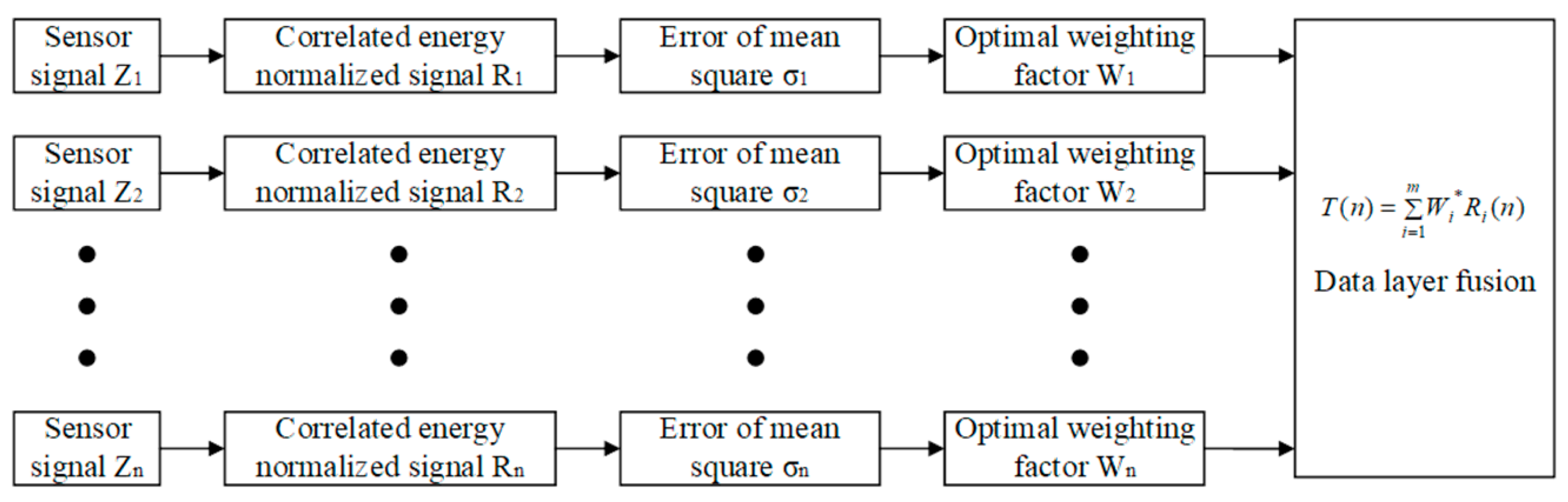
To fully use the subtle information and features of the original sensor data, this section combined correlation and adaptive weighting methods to perform the data layer fusion of the multi-source homogeneous sensor information. Firstly, the correlation signal energy function was constructed and normalized. Secondly, according to the conditions of the adaptive weighting method (i.e., the total mean square error was the minimum), the optimal weighting factor among sensors was adjusted adaptively [16], the fused signal reached the optimum, and the dynamic fusion of multi-source homogeneous sensor information is realized.
The flow chart of data layer fusion, multi-source homogeneous sensor information based on the correlation adaptive weighting method, is shown in Figure 3.
Let X ( n ) and Y ( n ) to be deterministic signals collected by sensors X and Y , then, the correlation function between signal X ( n ) and Y ( n ) could be acquired as shown in Equation (1).
R X Y = n = 0 X ( n ) Y ( n )
Suppose there were m homogeneous sensor signals Z 1 ( n ) , Z 2 ( n ) , , Z m ( n ) , the cross-correlation function between any two signals was shown as Equation (2).
R Z i Z j ( t ) = 1 n t t 0 = 1 n 1 Z i ( t 0 ) Z j ( t 0 + t )
where n was the number of data points of each signal, and t = 0 , 1 , 2 , , n 1 was the time series of the signal. The correlation energy of the discrete signals between two sensors is shown in Equation (3).
E i j = t = 0 n 1 [ R i j ( t ) ] 2
The correlation energy matrix of discrete signals between two sensors is shown in Equation (4).
E = 1 E 12 E 1 m E 21 1 E 2 m E m 1 E m 2 1
The correlation signal energy between the i th sensor and all homogeneous sensors is shown in Equation (5).
E i = j = 1 , j i m E i j
After normalizing E i , the normalized signal of correlation energy could be acquired, as shown in Equation (6).
R i ( n ) = Z i ( n ) E i
where Z i ( n ) was the data signal sequence collected by the i th sensor within time T , and R i ( 1 ) , R i ( 2 ) , , R i ( n ) were the correlation energy normalized discrete signals.
Let σ 1 , σ 2 , , σ m to be the mean square error of m sensor signals, respectively, after correlation energy normalization. Let T to be the true value after multi-sensor data fusion. Let W 1 , W 2 , , W m to be the weighting factor of weighted fusion of each sensor, respectively. Then, the gross mean square error of R i ( n ) ( i = 1 , 2 , , m ) was shown as Equation (7).
σ 2 = E [ i = 1 m W i 2 ( R R i ) 2 ] = i = 1 m W i 2 σ i 2
The weighting factor of each sensor satisfied Equation (8).
i = 1 m W i = 1
To make the weighting factor reach the optimal state and the total mean square error reach the minimum value, the minimum total mean square error was shown as Equation (9).
σ min 2 = i = 1 m 1 σ i 2
The optimal weighting factor could be obtained by combining Equations (7)–(9).
According to Equation (10), the multiple sensors signal fused by correlation weighted average could be acquired, as shown in Equation (11).
W i * = 1 σ i 2 i = 1 m σ i 2
T ( n ) = i = 1 m W i * R i ( n )

4. Feature Layer Fusion of Multi-Source Heterogeneous Sensors Based on 1D-CNN

To realize the feature layer fusion of motor multi-source heterogeneous sensor data, a multi-channel one-dimensional convolutional neural network model is first established in this paper. The model includes multiple submodels, and the hyperparameters of each submodel’s convolutional and pooling layers are the same. Secondly, the multi-source heterogeneous sensor data is used as the one-dimensional input of multiple sub-models. After multi-layer convolution and pooling processing, the data is input to Flatten layer to flatten the multi-channel one-dimensional data features. Finally, the flattened single-channel one-dimensional data features are input into the full-connection layer for data feature layer fusion.

4.1. One-Dimensional Convolutional Neural Network

Figure 4 shows the 1D-CNN network structure diagram, which includes the input, convolution, pooling, fully connected, and output layers [17].
In the input layer, the multi-source heterogeneous sensor information group acts as the input of the network. In the convolution layer, multiple groups of convolution kernel performed convolution operations to the previous layer’s output, extracted its information features and used a nonlinear activation function to output the results [18]. In the pooling layer, the output features of the convolution layer are screened and filtered using the pooling function, and the maximum or average value of the perception domain is obtained as the output feature map [19]. In the fully connected layer, the feature output of the previous layer is the input data of this layer, and the fully connected network is established using preset labels, which integrate the distinguished local features of the convolution layer and pooling layer. In the output layer, the previous layer’s output is calculated using the Softmax function [20], and the results are taken as the corresponding probability value of each category of labels, where the label corresponding to the maximum probability value was the final recognition result.

4.2. Experimental Platform Data Collection

The experiments in this paper are carried out on an experimental transmission platform of a three-phase asynchronous AC motor, which is arranged as shown in Figure 5. The experimental platform mainly includes a motor, reducer, torque sensor, eddy current brake, various sensors, and data acquisition card (model: USB2085, 16 channels analog input, the sampling frequency is the highest: 250 kHz). The sensors mainly include voltage sensors (range: 0–500 V, accuracy is 0.2%), current sensors (range: 0–10 A, accuracy is 0.2%), vibration sensors (range: 0–50 mm/s, sensitivity: 20 mv/mm/s, response frequency: 10–1000 Hz) and temperature sensor (range: 0–50 mm/s, accuracy: 0.2%). The platform collects various sensor data of the motor under different fault types as the input of the fault diagnosis model. We set a sample of 1 million data for each fault category.

4.3. Data Preprocessing

4.3.1. Data Slicing

To reduce the calculation steps and the time in the algorithm calculation, this paper uses the preprocessed original time domain data of the sensor as the input of the fault diagnosis model. The time domain diagram of the partial data of each sensor under different fault states is shown in Figure 6. From Figure 6, the data between different sensors in each fault state overlapped, and it is difficult to distinguish the fault features. So, the convolutional neural network should be used for deep mining. However, due to the large and complex amount of data in the data set, data should be sliced and processed. Taking 1000 sample points as a unit of length and slicing them, the original data points of each fault type are cut into 1000 wave data to make wave data with a length of 1, a width of 1000, and a depth of 6, which are used as the input of the neural network for training.

4.3.2. Data Labeling

In this paper, two identical motors and a pair of identical bearings with the motor bearings are prepared. The stator, rotor, and bearing of one of the motors are artificially damaged to simulate the possible failure of the parts caused by the motor in the running state. Meanwhile, according to the six fault types set in the paper (the stator fault, rotor fault, bearing outer ring fault, bearing inner ring fault, bearing rolling body fault, and the synthetic fault of the front and rear bearings [21]), the faulty parts are, respectively, replaced to another motor that works normally, to collect data on the six fault states and normal states of the motor. Each fault type corresponds to its label, as shown in Table 3. At the same time, the comparison experiment with the fault-free motor is carried out to verify whether the method could determine the motor fault type fast and accurately when applied to the actual working scene.

4.4. Model Building and Training

4.4.1. Model Building

The 1D-CNN model of the motor fault diagnosis is built in this paper based on the multi-sensor fusion, which consisted of six sub-models with the same parameters, each including an input layer and four convolution-averaging pooling layers. Multi-source heterogeneous sensor data as the input of each submodel and converted into a set of feature maps through the convolutional layer, then the feature mapping was down-sampled in the average pooling to reduce the number of parameters. Four convolutional-pooling layers are repeated, the output of the final pooling layer in each submodel is concatenated to a Flatten layer to flatten the multi-channel one-dimensional data features into a one-dimensional array, and then a fully-connected layer is used to perform feature fusion on the data features of multi-source heterogeneous sensor information. Then the information is passed to the Softmax function output layer. Finally, the probabilities of each fault category value are obtained, and one of the biggest probability categories was the recognition result. Figure 7 and Table 4 show the specific structure of the model and the main parameters of each structure.

4.4.2. Model Training

In this paper, the multi-source heterogeneous sensor information has been standardized and input into the established one-dimensional convolutional neural network model to train the model. The Relu function is used as the activation function to simplify the calculation process and avoid gradient disappearance. SGD (i.e., stochastic gradient descent method) is used to update the weights of each neural node in the neural network. The Softmax function is used as the classification function of the output layer. Moreover, the Dropout layer is introduced in the fully connected layer to avoid over-fitting [22]. At the same time, the Dropout layer can also be considered a product of noise and a fully connected matrix, thus guaranteeing the high robustness of the algorithm even under high-noise conditions.
In addition, the monitor system data set is divided into the training set and the test set according to the 4:1 scale. The learning rate was 0.1. The maximum number of iterations was 20. The batch size was 40, and every mini-batch training of the model would update the weights of each neural node.

4.5. Interpretation of Result

4.5.1. Model Evaluation Index

Accuracy, precision, and recall rates are the evaluation indexes of deep learning-based fault diagnosis models [23]. They are also used to evaluate the detection effect of diagnosis models. The accuracy rate is the ratio of the number of samples correctly classified by the classifier to the total number of samples. The precision rate is the ratio of the number of correctly classified samples to the number of predicted classified samples. The recall rate is the ratio of the number of samples correctly classified into the labels to the actual number of samples on the labels [24]. The formulas are shown in Equations (12)–(14).
A cc = T p + T N T P + F P + T N + F N
P = T P T P + F P
R = T P T P + F N
where T P is the number of correctly classified samples of a certain type of sample A, T N is the number of correctly classified samples of other types of samples, F P is the number of other type samples incorrectly classified as A , and F N is the number of incorrectly classified samples of a certain type of sample A.

4.5.2. Accuracy Rate and Loss Function Value

The total number of training samples of the model is 800, the number of mini-batch training samples is 20, then the training times of each iteration are 40. Since the total iteration times of the model are 20 times, its total training times are 800 times. Figure 8 shows the change in accuracy rate and loss function value (i.e., root mean square error) in the training process of the model aimed at the training set and the test set.
In the model’s training process, the training set’s accuracy rate increased steadily and converged to 99.3% with small fluctuations. The loss function value gradually decreased and approached 0. The fluctuation of the accuracy rate of the test set was obviously better than that of the training set, and the speeds of rising and convergence were faster. The loss function value was also closer to 0 than the training set. Therefore, this model had a significant effect on feature mining, fusion, classification, and diagnosis of the motor fault data.

4.5.3. Computational Time and Complexity of Algorithm Training

As one of the two performance evaluation indexes of the algorithm, time complexity qualitatively describes the algorithm’s running time, which is of great significance for the selection, construction, and optimization of the algorithm. For the convolutional neural network algorithm adopted in this paper, its time complexity is mainly reflected in the speed of the training process of the data set. If the complexity is excessive, the training time of the model will be long, resulting in a waste of time and economy. So it is of great significance to evaluate the algorithm’s time complexity.
According to the concept of time complexity of the convolutional neural network, its time complexity mainly includes the calculation amount of the convolutional layer and fully connected layer in the model. The time complexity calculation formula of a single convolutional layer is shown in Equation (15), and the time complexity calculation formula of a single fully connected layer is shown in Equation (16) [25]. Table 4 shows the specific structure of the one-dimensional convolutional neural network adopted in this paper. Therefore, this algorithm’s computational time and complexity during model training are shown in Table 5.
T ime ~ O ( M 2 K 2 C i n C o u t )
T ime ~ O ( ( 2 × C i n 1 ) C o u t )
where M2 is the area of the output feature map, K2 is the area of the convolution kernel, Cin is the number of input channels, and Cout is the number of output channels.

4.5.4. Comparison and Analysis with the Traditional Improved Model

The fault diagnosis model proposed in this paper is compared with the improved support vector machine method proposed in the cited literature study [26], the optimized BP neural network method proposed in the cited literature study [27], and the single-sensor 1D-CNN model analysis method. The accuracy rate and f1 score are shown in Table 6.
The cited study [26] proposed a new integrated SVM model, which applied KPCA in the support vector machine model to extract the critical information of the original data set, and the SVM was further trained. In this paper, three vibration signals of the motor were used as the sample set for training and testing, the RBF kernel function was used as the decision function to realize the nonlinear mapping of the fault features, and the genetic algorithm was used as the weight parameter optimization algorithm of SVM. After several training times, the accuracy rate of the model reached 63.08%.
The cited study [27] proposed an improved BP neural network, which applied the genetic algorithm to optimize the weight and threshold of the BP neural network, and the weight of each neural network node reached the optimum. In this paper, the three-layers network structure of the input layer, hidden layer, and output layer was adopted, the fully connected network was adopted to connect all the layers, and the Sigmoid function was used as the activation function to output its feature mapping. After numerous training and comparison, it was found that the nodes of each layer were set to 6, 12, and 7, and the diagnostic accuracy rate was the highest, 81.1%.
The single-sensor 1D-CNN fault diagnosis model had the same network structure and training parameters as the multi-sensor 1D-CNN fault diagnosis model aside from its single-channel input. The radial vibration signal of the front bearing was the network input in the single-sensor 1D-CNN fault diagnosis model, and its diagnosis accuracy rate was 86.29%.
As can be seen from Table 5, the accuracy and F1 score of the proposed fault diagnosis model in this article are 99.3% and 98.95%, respectively. Compared with the improved SVM, the improved BP neural network, and the single sensor convolutional neural network, the accuracy rate of the fault diagnosis model proposed in this paper is improved by 36.22%, 18.2%, and 13.01%, respectively. The F1 score is improved by 34.46%, 16.65%, and 11.05%, respectively. Therefore, the model in this paper has higher diagnosis efficiency and accuracy compared with the improved traditional motor fault diagnosis model.

5. Practical Fault Diagnosis Application

According to the concept of deep learning and the cited literature study [
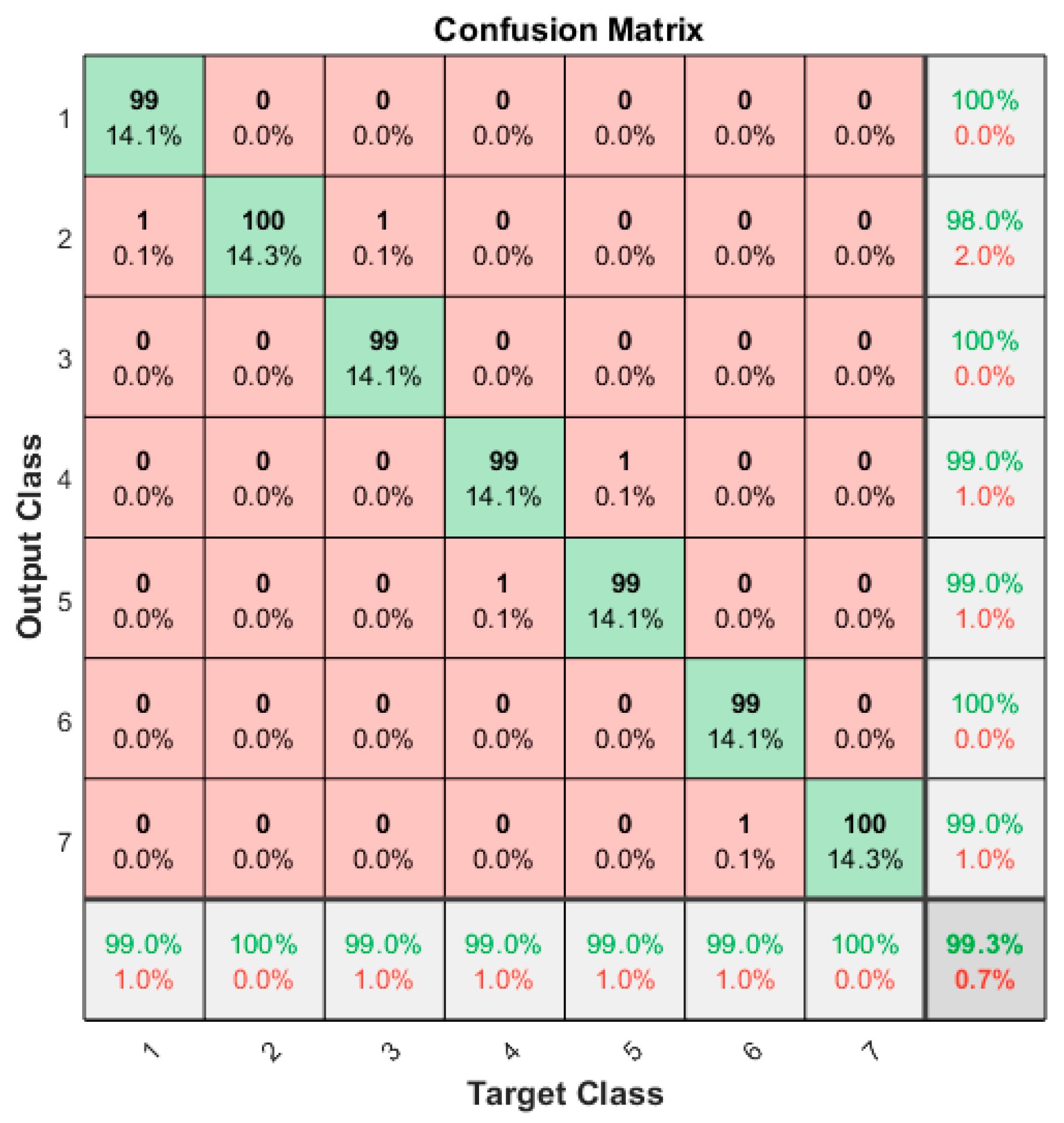
28], after the fault diagnosis model reaches the optimal convergence state through massive data training, blind data sets (unlabeled data sets) must be used to verify its diagnostic capability. In this section, the monitoring system data set (100 data of each fault are collected without labels) is input into the trained fault diagnosis model to verify further the feasibility and effectiveness of the model in the practical application of fault diagnosis. At the same time, the diagnosis results of the monitoring system data set are obtained and analyzed.
The confusion matrix of monitoring system data sets is shown in Figure 9, where the row represents predicting class (i.e., the output class), the columns represented the real class (i.e., the target class), and the diagonal line corresponds to the correct classification observations, and the off-diagonal corresponded to the misclassification observations, and the lower right corner of the cell showed the overall diagnostic accuracy rate, and the most right column was the precision and false discovery rate, and the bottom row was recall rate and false negative rate [29]. Each cell showed the percentage of the total observation number and frequency. From Figure 9, one sample was wrongly identified as other faults, respectively, in class 1, 3, 4, 5, and 6 faults. In contrast, the identification of other types of faults almost exactly corresponds to the real label with an accuracy rate of 99.3%.
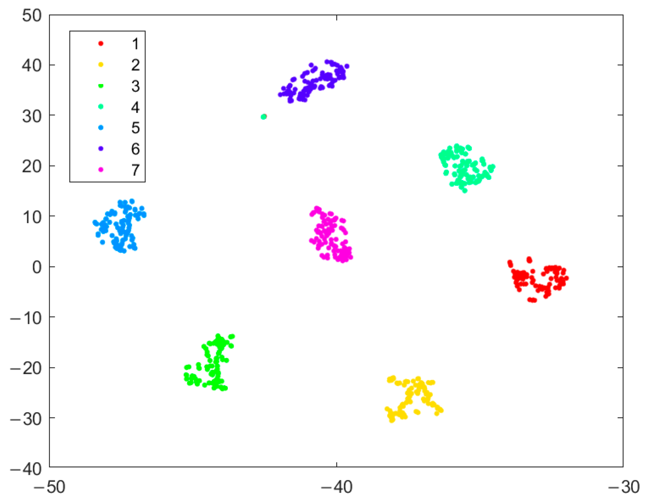
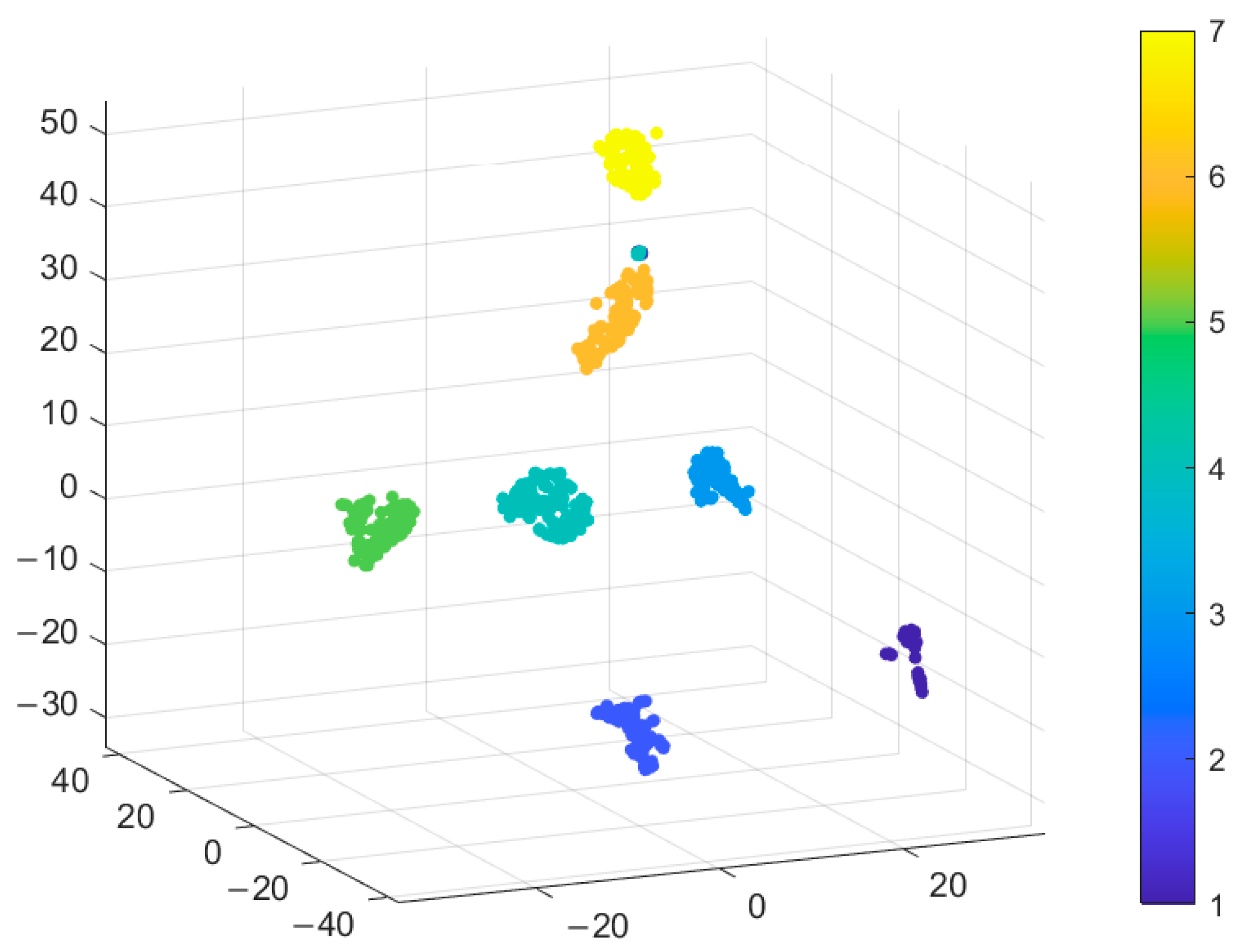
To observe the effect of diagnostic classification more intuitively, the output data of the fully connected layer in this model is taken out, the data are all reduced to two-dimensional and three-dimensional data by T-SNE, and then the clustering scatter diagram of classification results is drawn [30]. The 2D clustering scatter plot and the 3D clustering scatter plot are shown in Figure 10 and Figure 11, respectively. From the figures, the predicted values of each category are distinguished by different colors, the data points of the same color are concentrated in the same area, the data points of different colors are not mixed, and the distances are large. The classification results are accurate, which further showed that the method had a significant effect on motor fault diagnosis.
To sum up, the model has an excellent diagnostic effect in the actual application scenario of motor fault diagnosis. In the specified position of the motor, workers can install all kinds of sensors, and the multi-source sensor signals during the motor operation can be collected and inputted into the model proposed in this paper to realize the online fault diagnosis of the motor. In addition, to prevent possible misclassification of the model, a variable will be added when the model is deployed in real-time, which will store ten motor fault diagnosis results. When there are more than eight of the same diagnosis results, the diagnosis result will be output to the upper computer, and this variable will be cleared.

6. Conclusions

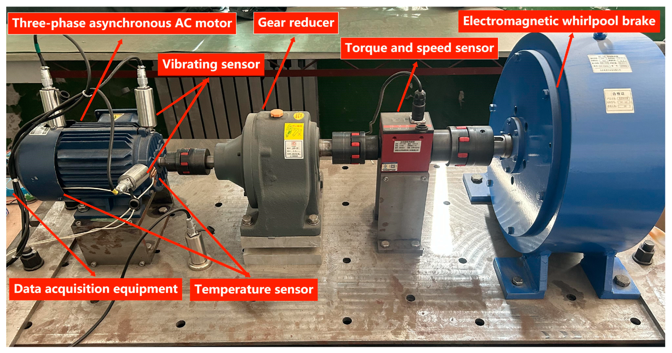
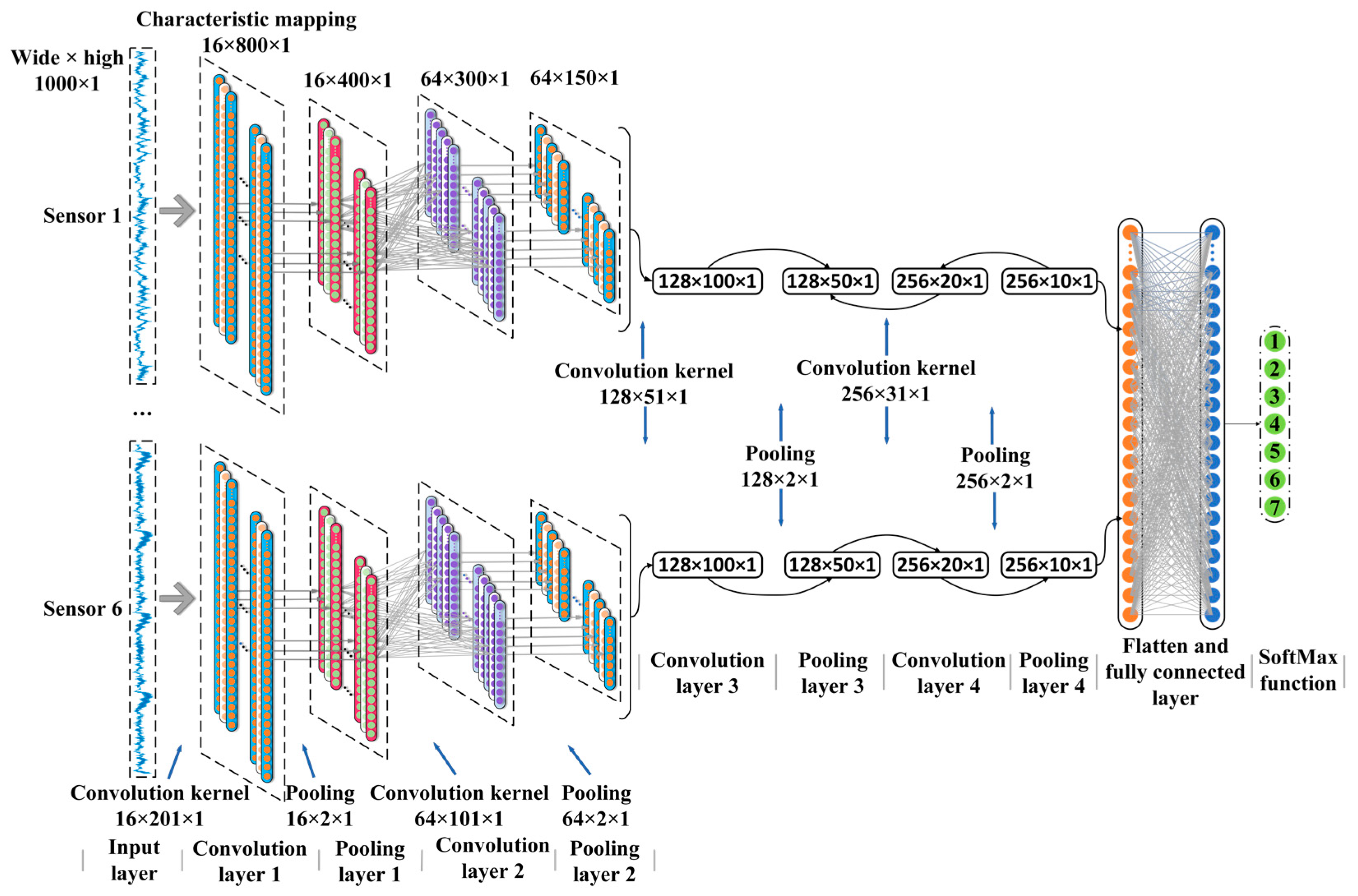
To improve the online fault diagnosis ability and accurately and efficiently identify the fault types in the running process of the motor, a fault diagnosis model combining multi-sensor data layer fusion and 1D-CNN multi-sensor feature layer fusion based on the correlation adaptive weighting method is proposed in this paper. Firstly, this paper proposes a correlation adaptive weighting method to fuse multi-source similar sensors information by the data layer. This method can retain a large amount of original data and provide the target with as fine information as possible to reduce the loss of fault features in the signal. Secondly, in this paper, a deep learning model (one-dimensional convolutional neural network) is adopted to carry out feature layer fusion of multi-source heterogeneous sensor information after data layer fusion, which can not only realize information compression and improve real-time performance but also maximize the characteristic information required for decision analysis. Finally, the proposed fault diagnosis model is tested on the experimental transmission platform of a three-phase asynchronous AC motor. The results are shown as follows:
  • The motor fault diagnosis model proposed in this paper, which is based on the combination of multi-sensor data layer fusion and feature layer fusion, could accurately identify the current fault category according to the collected multi-source sensor data with an accuracy rate of 99.3%.
  • Compared with traditional fault diagnosis methods based on single sensor and shallow learning, the multi-sensor information fusion diagnosis model based on deep learning had higher diagnosis efficiency and accuracy, and its fault diagnosis accuracy reached 99.3%. Compared with the improved SVM, BP neural network, and single sensor analysis method, the accuracy rate of this method is improved by 36.22%, 18.2%, and 13.01%, respectively.
  • After the data layer fusion of multi-source homogeneous sensors using the correlation adaptive weighting method was carried out, the fault information of multi-sensors could be fully extracted, which was conducive to improving the accuracy rate of fault diagnosis.
In this paper, multi-sensor data layer fusion, feature layer fusion, and deep learning algorithms are applied to motor fault diagnosis technology, which promoted the application of multi-information fusion and artificial intelligence technology in the field of motor fault diagnosis and intelligent operation and maintenance. Compared with the traditional fault diagnosis methods, the proposed method can accurately identify motor faults with simpler operation logic and higher efficiency.

Author Contributions

Conceptualization, Y.G.; methodology, Y.Z.; writing—review and editing, Y.Z.; funding acquisition, C.L.; supervision, M.Y.; formal analysis, Y.G. All authors have and editing, M.Y. All authors have read and agreed to the published version of the manuscript.

Funding

This research was funded by the [China Postdoctoral Science Foundation] grant number [2021M700529], [Natural Science Basic Research Program of Shaanxi Province] grant number [2022JQ-434], [Fundamental Research Funds for the Central Universities] grant number [300102252110].

Institutional Review Board Statement

Not applicable.

Informed Consent Statement

Not applicable.

Data Availability Statement

The experimental data used in this paper are from the autonomous measurement of the autonomous driving and maglev technology equipment team of Chang’an University.

Acknowledgments

The authors are very grateful for all the constructive comments that helped us improve the original version of the manuscript.

Conflicts of Interest

The authors declare no conflict of interest.

Abbreviation

Symbols/AbbreviationsFull Name/Meaning
1D-CNNOne-Dimensional Convolutional Neural Network
SVMSupport Vector Machine
NN classifierNeural Network Classifier
MDFMulti-sensor Data Fusion
(ADCNN)Adaptive convolutional neural network
VVolt
AAmpere
mm/sMillimeters per Second
°CDegree Centigrade
ACAlternating Current
1D arrayone-dimensional array
SGDStochastic Gradient Descent

References

  1. De las Morenas, J.; Moya-Fernández, F.; López-Gómez, J.A. The Edge Application of Machine Learning Techniques for Fault Diagnosis in Electrical Machines. Sensors 2023, 23, 2649. [Google Scholar] [CrossRef] [PubMed]
  2. Dineva, A.; Mosavi, A.; Gyimesi, M.; Vajda, I.; Nabipour, N.; Rabczuk, T. Fault Diagnosis of Rotating Electrical Machines Using Multi-Label Classification. Appl. Sci. 2019, 9, 5086. [Google Scholar] [CrossRef] [Green Version]
  3. Chang, H.-C.; Wang, Y.-C.; Shih, Y.-Y.; Kuo, C.-C. Fault Diagnosis of Induction Motors with Imbalanced Data Using Deep Convolutional Generative Adversarial Network. Appl. Sci. 2022, 12, 4080. [Google Scholar] [CrossRef]
  4. Mehrdad, H.; Mohsen, Z.; Mehrdad, N.; Bilal, A. A Wavelet-Based Fault Diagnosis Approach for Permanent Magnet Synchronous Motors. IEEE Trans. Energy Convers. 2019, 34, 761–772. [Google Scholar]
  5. Kerboua, A.; Metatla, A.; Kelailia, R.; Batouche, M. Fault Diagnosis in Induction Motor using Pattern Recognition and Neural Networks. In Proceedings of the International Conference on Signal, Image, Vision and their Applications (SIVA), Guelma, Algeria, 26–27 November 2018; pp. 1–7. [Google Scholar]
  6. Kale, A.P.; Wahul, R.M.; Patange, A.D.; Soman, R.; Ostachowicz, W. Development of Deep Belief Network for Tool Faults Recognition. Sensors 2023, 23, 1872. [Google Scholar] [CrossRef]
  7. Kerboua, A.; Metatla, A.; Kelaiaia, R.; Mohamed, B. Real-time safety monitoring in the induction motor using deep hierarchic long short-term memory. Int. J. Adv. Manuf. Technol. 2018, 99, 2245–2255. [Google Scholar] [CrossRef]
  8. Patil, S.S.; Pardeshi, S.S.; Patange, A.D. Health Monitoring of Milling Tool Inserts Using CNN Architectures Trained by Vibration Spectrograms. CMES-Comput. Model. Eng. Sciences. 2023, 136, 177–199. [Google Scholar] [CrossRef]
  9. Junior, R.F.R.; Dos Santos Areias, I.A.; Campos, M.M.; Teixeira, C.E.; Da Silva, L.E.B.; Gomes, G.F. Fault detection and diagnosis in electric motors using 1d convolutional neural networks with multi-channel vibration signals. Measurement 2022, 190, 110759. [Google Scholar] [CrossRef]
  10. Cheng, L.; Lu, J.; Li, S.; Ding, R.; Xu, K.; Li, X. Fusion Method and Application of Several Source Vibration Fault Signal Spatio-Temporal Multi-Correlation. Appl. Sci. 2021, 11, 4318. [Google Scholar] [CrossRef]
  11. Wang, X.; Mao, D.; Li, X. Bearing fault diagnosis based on vibro-acoustic data fusion and 1D-CNN network. Measurement 2021, 173, 108518. [Google Scholar] [CrossRef]
  12. Jing, L.; Wang, T.; Zhao, M.; Wang, P. An Adaptive Multi-Sensor Data Fusion Method Based on Deep Convolutional Neural Networks for Fault Diagnosis of Planetary Gearbox. Sensors 2017, 17, 414. [Google Scholar] [CrossRef] [PubMed] [Green Version]
  13. Zhang, W.; Peng, G.; Li, C. A New Deep Learning Model for Fault Diagnosis with Good Anti-Noise and Domain Adaptation Ability on Raw Vibration Signals. Sensors 2017, 17, 425. [Google Scholar] [CrossRef] [PubMed] [Green Version]
  14. Shao, Y.; Yuan, X.; Zhang, C.; Song, Y.; Xu, Q. A Novel Fault Diagnosis Algorithm for Rolling Bearings Based on One-Dimensional Convolutional Neural Network and INPSO-SVM. Appl. Sci. 2020, 10, 4303. [Google Scholar] [CrossRef]
  15. Yi, C.; Xin, L.; Hai, Z.; Jun, W.; Hai, S.; Hua, D. A novel hierarchical structural pruning-multiscale feature fusion residual network for intelligent fault diagnosis. Mech. Mach. Theory. 2023, 184, 105292. [Google Scholar]
  16. Shi, J.; Ren, Y.; Tang, H.; Xiang, J. hydraulic directional valve fault diagnosis using a weighted adaptive fusion of multi dimensional features of a multi-sensor. J. Zhejiang Univ.-Sci. A (Appl. Phys. Eng.) 2022, 23, 257–272. [Google Scholar] [CrossRef]
  17. Swapnil, K.G.; Prasad, V.K. Bearing fault diagnosis using time segmented Fourier synchrosqueezed transform images and convolution neural network. Measurement 2022, 203, 111855. [Google Scholar]
  18. Jia, F.; Li, S.; Shen, J.; Ma, J.; Li, N. Fault Diagnosis of Rolling Bearings Using Deep Transfer Learning and Adaptive Weighting. J. Xi’an Jiaotong Univ. 2022, 56, 1–10. [Google Scholar]
  19. Jiang, G.; He, H.; Yan, J.; Xie, P. Multiscale Convolutional Neural Networks for Fault Diagnosis of Wind Turbine Gearbox. IEEE Trans. Ind. Electron. 2019, 66, 3196–3207. [Google Scholar] [CrossRef]
  20. Krizhevsky, A.; Sutskever, I.; Hinton, E.G. ImageNet classifification with deep convolutional neural networks. Adv. Neural Inf. Process. Syst. 2012, 25, 1097–1105. [Google Scholar]
  21. Han, J.-H.; Choi, D.-J.; Hong, S.-K.; Kim, H.-S. Motor Fault Diagnosis Using CNN Based Deep Learning Algorithm Considering Motor Rotating Speed. In Proceedings of the 6th International Conference on Industrial Engineering and Applications (ICIEA), Tokyo, Japan, 12–15 April 2019; pp. 440–445. [Google Scholar]
  22. Liu, Y.; Yan, X.; Zhang, C.-A.; Liu, W. An Ensemble Convolutional Neural Networks for Bearing Fault Diagnosis Using Multi-Sensor Data. Sensors 2019, 19, 5300. [Google Scholar] [CrossRef] [Green Version]
  23. Abd-Elhay, A.-E.R.; Murtada, W.A.; Youssef, M.I. A Reliable Deep Learning Approach for Time-Varying Faults Identification: Spacecraft Reaction Wheel Case Study. IEEE Access 2022, 10, 75495–75512. [Google Scholar] [CrossRef]
  24. Deng, X.; Liu, Q.; Deng, Y.; Mahadevan, S. An improved method to construct basic probability assignment based on the confusion matrix for classification problem. Inf. Sci. 2016, 340–341, 250–261. [Google Scholar] [CrossRef]
  25. Shahid, S.M.; Ko, S.; Kwon, S. Performance Comparison of 1D and 2D Convolutional Neural Networks for Real-Time Classification of Time Series Sensor Data. In Proceedings of the International Conference on Information Networking (ICOIN), Jeju-si, Republic of Korea, 11–14 January 2022; pp. 507–511. [Google Scholar]
  26. Li, J. A Novel Integrated SVM for Fault Diagnosis Using KPCA and GA. J. Phys. Conf. Ser. 2019, 1207, 1. [Google Scholar]
  27. Liu, P.; Zhang, W. A Fault Diagnosis Intelligent Algorithm Based on Improved BP Neural Network. Int. J. Pattern Recognit. Artif. Intell. 2019, 33, 9. [Google Scholar] [CrossRef]
  28. Bajaj, N.S.; Patange, A.D.; Jegadeeshwaran, R.; Pardeshi, S.S.; Kulkarni, K.A.; Ghatpande, R.S. Application of metaheuristic optimization based support vector machine for milling cutter health monitoring. Intell. Syst. Appl. 2023, 18, 200196. [Google Scholar] [CrossRef]
  29. Duan, S.; Huang, P.; Chen, M.; Wang, T.; Sun, X.; Chen, M. Semi-supervised classification of fund-us images combined with CNN and GCN. J. Appl. Clin. Med. Phys. 2022, 23, e13746. [Google Scholar] [CrossRef]
  30. Kimura, M. Generalized T-SNE Through the Lens of Information Geometry. IEEE Access 2021, 9, 129619–129625. [Google Scholar] [CrossRef]
Figure 3. Data layer fusion flow chart of multi-source homogeneous information.
Applsci 13 04192 g003
Figure 4. Structure diagram of one-dimensional convolutional neural network.
Applsci 13 04192 g004
Figure 5. Transmission experimental platform of three-phase asynchronous AC motor.
Applsci 13 04192 g005
Figure 6. Time domain diagram of data under different fault states.
Applsci 13 04192 g006
Figure 7. One-dimensional convolutional neural network model for multi-sensor fusion.
Applsci 13 04192 g007
Figure 8. Change of model’s accuracy rate and loss function value.
Applsci 13 04192 g008
Figure 9. Confusion matrix.
Applsci 13 04192 g009
Figure 10. Two-dimensional cluster scatter diagram.
Applsci 13 04192 g010
Figure 11. Three-dimensional cluster scatter diagram.
Applsci 13 04192 g011
Table 1. Composition of multi-source homogeneous information of motor.
Homogeneous Sensor InformationSignalUnits
Multi-source similar information 1Phase A voltage of motor UaV
Phase A voltage of motor UbV
Phase A voltage of motor UcV
Multi-source similar information 2Stator phase A current IaA
Stator phase A current IbA
Stator phase A current IcA
Multi-source similar information 3Rotor vibrates horizontally Vhmm/s
Rotor vibrates vertically Vvmm/s
Multi-source similar information 4A phase winding temperature Ta°C
A phase winding temperature Tb°C
A phase winding temperature Tc°C
Table 2. Composition of multi-source heterogeneous information of motor.
Heterogeneous Sensors InformationSignalUnits
Multi-source heterogeneous information 1Fusion stator voltage UeV
Multi-source heterogeneous information 2Fusion stator current IeA
Multi-source heterogeneous information 3Fusion bearing vibration Vemm/s
Multi-source heterogeneous information 4Fusion temperature Te°C
Multi-source heterogeneous information 5Rear bearing vibration Vamm/s
Multi-source heterogeneous information 6Stator temperature Tf°C
Table 3. Labeling of motor fault modes.
Sample Capacity
(Training Set/Test Set)
Sample WidthFault CategoryLabels
800/2001000Fault-free motor1
800/2001000Stator fault2
800/2001000Rotor fault3
800/2001000Bearing outer ring fault4
800/2001000Bearing inner ring fault5
800/2001000Bearing rolling body fault6
800/2001000Synthetic fault of the front and rear bearings7
Table 4. Specific structure parameters of the 1D-CNN model.
Level NumberLayer CategoriesNumber of Cores/Size/Step SizePostscript
1Input layer6 × 1000 × 1Channel × dimension
2Convolution layer16/201 × 1/1Relu
3Pooling layer16/2 × 1/1Average pooling
4Convolution layer64/101 × 1/1Relu
5Pooling layer64/2 × 1/1Average pooling
6Convolution layer128/51 × 1/1Relu
7Pooling layer128/2 × 1/1Average pooling
8Convolution layer256/31 × 1/1Relu
9Pooling layer256/2 × 1/1Average pooling
10Flatten layer256
11Fully connected layer256Relu
12Output layer7Softmax
Table 5. The computational time and complexity of this algorithm during model training.
Number of Epochs in Model TrainingComputation TimeTime Complexity
1 epoch108 s 14 ms104397312
20 epoch36 min 4 s 54 ms2087946240
Table 6. Accuracy rate and loss function value.
Model NameAccuracy RateF1 Score
Multi-sensor 1D-CNN model99.3%98.95%
Support Vector Machine (SVM)63.08%64.49%
BP neural network81.1%82.3%
Single-sensor 1D-CNN model86.29%87.9%
Disclaimer/Publisher’s Note: The statements, opinions and data contained in all publications are solely those of the individual author(s) and contributor(s) and not of MDPI and/or the editor(s). MDPI and/or the editor(s) disclaim responsibility for any injury to people or property resulting from any ideas, methods, instructions or products referred to in the content.

