Simultaneous Fault Diagnosis Based on Hierarchical Multi-Label Classification and Sparse Bayesian Extreme Learning Machine

Abstract

This paper proposes an intelligent simultaneous fault diagnosis model based on a hierarchical multi-label classification strategy and sparse Bayesian extreme learning machine. The intelligent diagnosis model compares the similarity between an unknown sample to be diagnosed and each single fault mode, then outputs the probability of each fault mode occurring. First, multiple two-class sub-classifiers based on SBELM are trained by using single-fault samples to extract the correlation between various pairs of single-fault, and the sub-classifiers are integrated with the proposed hierarchical multi-label classification (HMLC) strategy to form the diagnostic model based on HMLC-SBELM. Then, samples of single faults and simultaneous faults are used to generate the optimal discriminative thresholds by using optimization algorithms. Finally, the probabilistic output generated by the HMLC-SBELM-based model is transformed into the final fault modes by using the optimal discriminative threshold. The model performance is evaluated by using actual vibration signals of the main reducer and is compared with several classical models. The contrastive results indicate that the proposed model is more accurate, efficient, and stable.

1. Introduction

In the main reducer assembly of automobiles, about 80% of the failures occur in the paired gear system [1,2]. So intelligent real-time monitoring systems can identify the fault gear in a timely fashion, and effectively identify the paired gear fault type. It not only can reduce the scrap rate and decrease rework to reduce production costs, also can reduce the vibration level to improve the working performance of the transmission system and eventually improve the comfort and safety of the car [3,4].

Due to the complicated assembling process of the main reducer assembly and the complex internal structure, the correlation between each component is very close which results in multi-level failure. So when a function fails inside the main reducer, it may be due to a single fault or multiple faults occurring at the same time [5,6,7,8].

Benefiting from the increasing development and gradual maturity of machine learning and deep learning technologies, intelligent diagnosis of machinery has achieved more breakthroughs, especially in the field of simultaneous fault diagnosis. Yunpu Wu utilized Bayesian deep learning and between-class learning to create a simultaneous fault diagnosis model [9]. Pengfei Liang utilized GAN and time-frequency imaging technology for simultaneous fault diagnosis of gearbox [10]. Yanghui Tan contributed comparative research on several simultaneous fault diagnosis methods based on multi-label classification [11]. Samira Zare used convolutional neural networks to diagnose the simultaneous fault of a wind turbine [12].

Although these researches have achieved satisfactory results, most of the achievements adopted single-label classification to solve simultaneous fault diagnosis. That is, each sample belongs to only one category, and each simultaneous fault type is processed as a special new single-fault type. Furthermore, a diagnostic model based on single-label classification requires a great many simultaneous failure samples to train the diagnostic model. Generally speaking, the principal difficulties of identifying simultaneous fault are arranged as follows:

(1)

Simultaneous fault is not a simple combination of multiple single faults, so it is unfeasible to use a simple and traditional model of mechanism to recognize simultaneous faults.

(2)

In practice, due to the high number of species of all possible simultaneous failure modes, it is impractical to collect ample samples of all simultaneous failure modes to train a fault classification model focused on both single failure modes and simultaneous failure modes recognition.

(3)

There is no one-to-one correspondence between failure signs and failure cause, and the failure signs have the characteristics of large ambiguity, strong coupling, and uncertainty, which further increase the difficulty of recognition.

To tackle the above-mentioned challenges, diagnostic models for single and simultaneous faults must be capable of probabilistic classification, which can clearly reflect the probability of various single fault types. The extreme learning machine (ELM) organizes multiple neurons in a three-layer structure, and the data transmission direction of the neural network is forward [13,14]. The characteristics of ELM include short training time and simple operation. The classification capability of ELM is superior to that of the BP network and support vector machine (SVM), and its execution time is significantly shorter than that of SVM [15,16]. Wong P K et al. used ELM to diagnose failures in real-time for power generation systems in power plants [17]. Tian Ye combined singular value decomposition with ELM in [18]. By combining ELM with an optimized sample entropy algorithm, Yuedong Song et al. proposed an automatic recognition system [19]. Huang Guang-Bin utilized ELM into the regression and classification problem [20].

At present, there are many derivative algorithms based on ELM. Emilio Soria-Olivas introduced the Bayesian method into ELM to create Bayesian ELM (BELM). BELM estimated the output probability distribution to optimize the output weights of the network and is used to solve linear regression problems [21,22,23]. Sparse Bayesian ELM (SBELM) [24] combined the sparse Bayesian theory with ELM to achieve a sparse representation of output weight by setting a hyperparameter for each hidden layer output weight. SBELM not only possess excellent learning ability but is also able to output probabilistic results [25].

In addition, the best solution to improve the limitation of single-label classification in simultaneous fault recognition is to use multi-label classification, which defines an m-dimensional vector for the category label of each sample and trains the intelligent diagnostic model using samples of single fault types [26,27,28]. In order to identify simultaneous fault types in the fault diagnosis process, the diagnostic model must be able to provide the probability of all single fault types. The probability output is used to judge and identify the simultaneous fault types according to the ranking of the probability.

Considering the superiority of SBELM, this paper proposes a simultaneous fault diagnosis framework based on hierarchical multi-label classification and SBELM. The function of the diagnostic mechanism of the proposed framework is to compare the similarity between the unknown sample to be diagnosed and each single fault mode, which is measured by the Bayesian-based probabilistic output.

The principal contributions of this paper are as follows:

(1)

A simultaneous fault diagnosis framework based on a hierarchical multi-label classification strategy and a feed-forward neural network based on sparse Bayesian is proposed to effectively recognize single failures and simultaneous failures. Only single failure samples are participating in the training procedure of the model.

(2)

There is a certain correlation between each pair of single faults, to improve the classification accuracy, this paper introduces paired strategy into multi-label classification to create a hierarchical multi-label classification model.

(3)

The proposed diagnostic framework is utilized for the intelligent fault diagnosis of the main reducer. When simultaneous fault exists, it’s achievable to accurately identify multiple single faults that occur at the same time. The experimental results indicate that the framework performance is superior in recognition accuracy.

2. The Fundamental Theories

2.1. Extreme Learning Machine (ELM)

Given N samples D = (x_i, t_i), i = 1,…,N, in which x_i ∈ Rⁿ, t_i ∈ R^m represents the class label of x_i, and m is the number of class labels. The output function of an extreme learning machine with L hidden layer nodes is expressed as:

$$f\left(\mathrm{x}\right)={{\displaystyle \sum }}_{i=1}^L{\beta }_i{h}_i\left(a_i,b_i,x\right)=\beta ·H\left(x\right)$$

(1)

in which a_i represents input weights between input layer and the ith hidden layer node, b_i represents the bias of the ith hidden layer node, h_i (∙) is the activation function of the hidden layer. β = [β₁,…, β_L]^T represents output weights, and H(x) = [h₁ (a₁,b₁,x),…,h_L (a_L,b_L,x)] is the output matrix of the hidden layer in which each element h_i (a_i,b_i,x) is the output of the ith hidden layer nodes. The above formula is expressed as:

Hβ = T

(2)

in which T is the class label matrix of sample set D. H represents the feature mapping matrix as shown as follows:

$$H=\left[\begin{array}{ccc}{h}_1\left(a_1,b_1,x_1\right)& \cdots & h_L\left(a_L,b_L,x_1\right)\\ ⋮& \ddots & ⋮\\ h_1\left(a_1,b_1,x_N\right)& \cdots & h_L\left(a_L,b_L,x_N\right)\end{array}\right]$$

(3)

According to the orthogonal projection method [29], the Moore-Penrose generalized inverse H^† [30] of matrix H is obtained to calculate the output weights β:

$$\beta =H^{†}T, H^{†}={\left(H^{T}H\right)}^{-1}{H}^T$$

(4)

The three-step learning process of ELM is: (1) randomly generate the input weight a and bias b of L hidden layer nodes; (2) calculate the feature mapping matrix H; (3) calculate the output weight β according to H^†.

2.2. Sparse Bayesian Extreme Learning Machine (SBELM)

SBELM learns the output weights by using Bayesian inference. For a two-class classification problem, the probability of each training sample is expressed as P(t|x). The likelihood function can be represented as:

$$\mathrm{P}\left(t|\beta ,h\right)={{\displaystyle \prod }}_{i=1}^N\sigma {\left[y\left(h_i,\beta \right)\right]}^{t_i}{\left(1-\sigma \left[y\left(h_i,\beta \right)\right]\right)}^{1-t_i}$$

(5)

where $y\left(h_i,\beta \right)=h\beta$, $t={\left(t_1,\dots ,t_N\right)}^T$ is the class label of N samples in which $t_i \in \left\{0,1\right\}$ and σ(∙) represents sigmoid function as follows:

$$\sigma \left[y\left(h_i,\beta \right)\right]=1/\left(1+e^{-y\left(h_i,\beta \right)}\right)$$

(6)

The output weight ${\beta }_i$ obeys Gaussian conditional probability distribution with a mean of 0 and a variance of $a_i{}^{-1}$:

$$\mathrm{P}\left({\beta }_i|{\alpha }_i\right)=\mathcal{N}\left({\beta }_i|0,a_i{}^{-1}\right), \alpha ={\left[{\alpha }_1,\dots ,{\alpha }_L\right]}^T$$

(7)

$$\mathrm{P}\left(\beta |\alpha \right)={{\displaystyle \prod }}_{i=1}^L\frac{{\alpha }_i}{\sqrt{2\pi }}\exp \left(-\frac{{\alpha }_i{\beta }_i^2}{2}\right)$$

(8)

where $\alpha$ is the hyper-parameter to determine the prior distribution of $\beta$. The key task is to focus on the marginal likelihood distribution $\mathrm{P}(t|\alpha ,H)$ of output t on condition of $\alpha$ and H. The parameters $\alpha$ can be obtained by maximizing the marginal likelihood using the Laplace approximation approach.

Generally, the iterative reweighted least squares algorithm (IRLS) is used to calculate the mean value of the Gauss distribution ${\beta }_{MP}$. To update ${\beta }_{MP}$, gradient $\nabla \mathrm{E}$ and Hessian matrix $\mathsf{\Phi }$ are calculated firstly:

$$\nabla \mathrm{E} ={\nabla }_{\beta }\log \left\{P\left(t|\beta ,H\right)P\left(\beta |\alpha \right)\right\}=H^{\mathrm{T}}\left(t-y\right)-A\beta$$

(9)

$$\mathsf{\Phi } ={\nabla }_{\beta }{\nabla }_{\beta }\log \left\{P\left(t|\beta ,H\right)P\left(\beta |\alpha \right)\right\}=-\left(H^{\mathrm{T}}BH+A\right)$$

(10)

$$A=\mathrm{diag}\left(a\right)$$

(11)

where $\mathrm{y} ={\left(y_1,\dots ,y_N\right)}^T$ represents the predicted output of N samples, B represents the diagonal matrix and $b_i=y_i\left(1-y_i\right)$. According to IRLS, ${\beta }_{MP}$ is updated as follows:

$${\beta }_{MP}={\beta }_{MP}-{ \mathsf{\Phi }}^{-1}\nabla \mathrm{E} ={\left(H^{T}BH+A\right)}^{-1}{H}^{T}B\widehat{t}$$

(12)

where $\widehat{t }=H\beta +B^{-1}\left(t-y\right)$. ${\beta }_{MP}$ and ${{\displaystyle \sum }}^{ }$ of the weight parameter Gauss distribution which is approximated using the Laplace approximation method can be expressed as:

$${{\displaystyle \sum }}^{ }={\left(H^T\mathrm{BH} + \mathrm{A}\right)}^{-1}$$

(13)

$${\beta }_{MP}={{\displaystyle \sum }}^{ }{H}^{T}B\widehat{t}$$

(14)

After obtaining the Gauss distribution of weight parameter $\beta$, the logarithm of the marginal likelihood function is expressed as:

$$ℒ\left(a\right)=\log P(t|a,H)$$

(15)

Calculate the partial derivative of $ℒ\left(a\right)$ to the hyper-parameter $a$ and set the value to 0:

$$\frac{\partial ℒ\left(a\right)}{\partial a_i}=\frac{1}{2a_i}-\frac{1}{2}{\mathsf{\Sigma }}_{ii}-\frac{1}{2}{\beta }_{M{P}_i}{}^2=>a_i{}^{new}=\frac{1-a_i{\mathsf{\Sigma }}_{ii}}{{\beta }_{M{P}_i}{}^2}$$

(16)

Using Formula (16), most of $a_i$ tends to infinity, and its corresponding weight ${\beta }_i$ tends to 0. The hidden layer nodes with a weight of 0 are deleted to achieve the sparseness of hidden layer nodes. With the sparse hidden layer weight vector ${\beta }^{\prime }$, predict the probability of unknown sample $x_{new}$ using $\mathrm{y}\left(h,{\beta }^{\prime }\right)=h{\beta }^{\prime }$:

$$\mathsf{\sigma }\left[\mathrm{y}\left(h,{\beta }^{\prime }\right)\right]=1/\left(1+e^{-\mathrm{y}\left(h,{\beta }^{\prime }\right)}\right)$$

(17)

3. Proposed Methodology

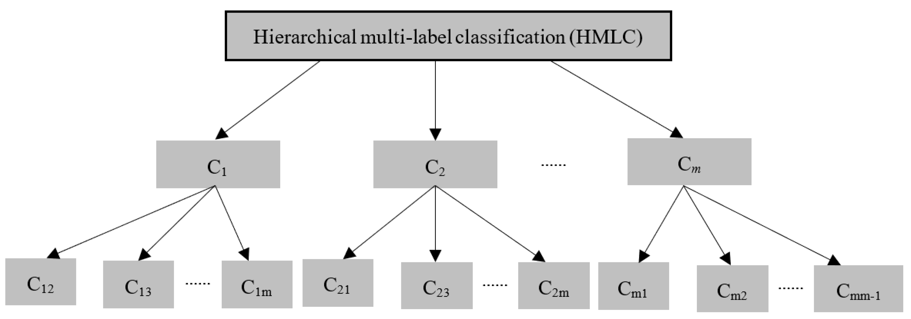
3.1. Design of Hierarchical Multi-Label Classification Strategy

The occurrence of simultaneous failure means that multiple different single failure modes break out at the same time, and the category label necessarily contains multiple various elements representing the corresponding single failure modes. Simultaneous fault identification not only has the characteristics of multi-label but also has the characteristics of multi-class. The most frequently used methods to solve multi-class classification problems are summarized below:

(1)

Calculate the occurrence probability of all categories, and the category corresponding to the maximum value is chosen as the prediction category;

(2)

Based on binary classification, the classification problem with multiple classes can be skillfully converted into several sub-problems with two classes to be solved, and then the multiple binary classification results are effectively combined.

Considering the lack of ample simultaneous fault samples, this paper proposes a novel hierarchical multi-label classification strategy as shown in Figure 1. The hierarchical multi-label classification strategy solves the classification problem with multi-class by combining a series of sub-classifiers.

As shown in Figure 1, at the first level, each classifier only focuses on the identification of one fault category. For diagnostic problems with m fault types, there are m classifiers presented as [C₁, C₂, …, C_m] in which C_i is utilized to recognize the ith fault type. At the second level, each classifier at the previous level is segmented into several sub-classifiers which can be trained by single fault samples. Such as, the ith classifier Ci in the first level is further expressed as dichotomization [C_i1, C_i2, …, C_im] (m ≠ i) in which m − 1 element represents a set of sub-classifiers focusing on two classes.

3.2. Design of Hierarchical Multi-Label Classification Strategy

SBELM has the characteristic of probability output. By calculating the predicted probability distribution of an unknown sample x, the fault diagnosis algorithm based on SBELM can provide a conditional probability of all failures for sample x, that is, to achieve the probability output.

For simultaneous fault diagnosis, any two single failure modes may have some correlation between them. Since the traditional SBELM can only be used to solve the classification problem of two classes. To address the multi-class classification problem, this paper combines the proposed hierarchical multi-label classification strategy (HMLC) with SBELM to construct the model based on HMLC-SBELM. The architecture of the model based on HMLC-SBELM is shown in Figure 2.

The model is constructed of m combinational SBELM (C-SBELM) which can be expressed as [C-SBELM₁, C-SBELM₂, …, C-SBELM_m]. That is, the simultaneous fault diagnosis model based on HMLC-SBELM outputs a probabilistic vector [p₁, p₂, …, p_m] in which each element pi is the output of C-SBELMi th to measure the occurrence possibility of the ith fault mode. According to the strategy of HMLC, C-SBELMi is composed of m-1 independent two-class sub-classifiers [SBELM_i1, SBELM_i2, …, SBELM_im], and each classifier SBELM_ij is trained by training samples of the ith fault and training samples of jth fault. The output of SBELM_ij is expressed as p_ij which is used to judge the probability that an unknown sample belongs to the ith or the jth fault mode.

Due to the complementarity between SBELM_ij and SBELM_ji, that is, p_ij = 1 − p_ji, the diagnostic model based on HMLC-SBELM contains m(m − 1)/2 two-class sub-classifiers. For an unknown sample x, SBELM_ij can predict the possibility of associating the category ti for sample x. It means that the output of SBELM_ij is a conditional probability $p_{ij}(t_i|x,{\beta }^{\prime })$.

The simultaneous fault diagnosis model based on HMLC-SBELM fully considers the correlation between any two single fault modes, thus enabling more accurate category probability estimates when performing simultaneous fault identification.

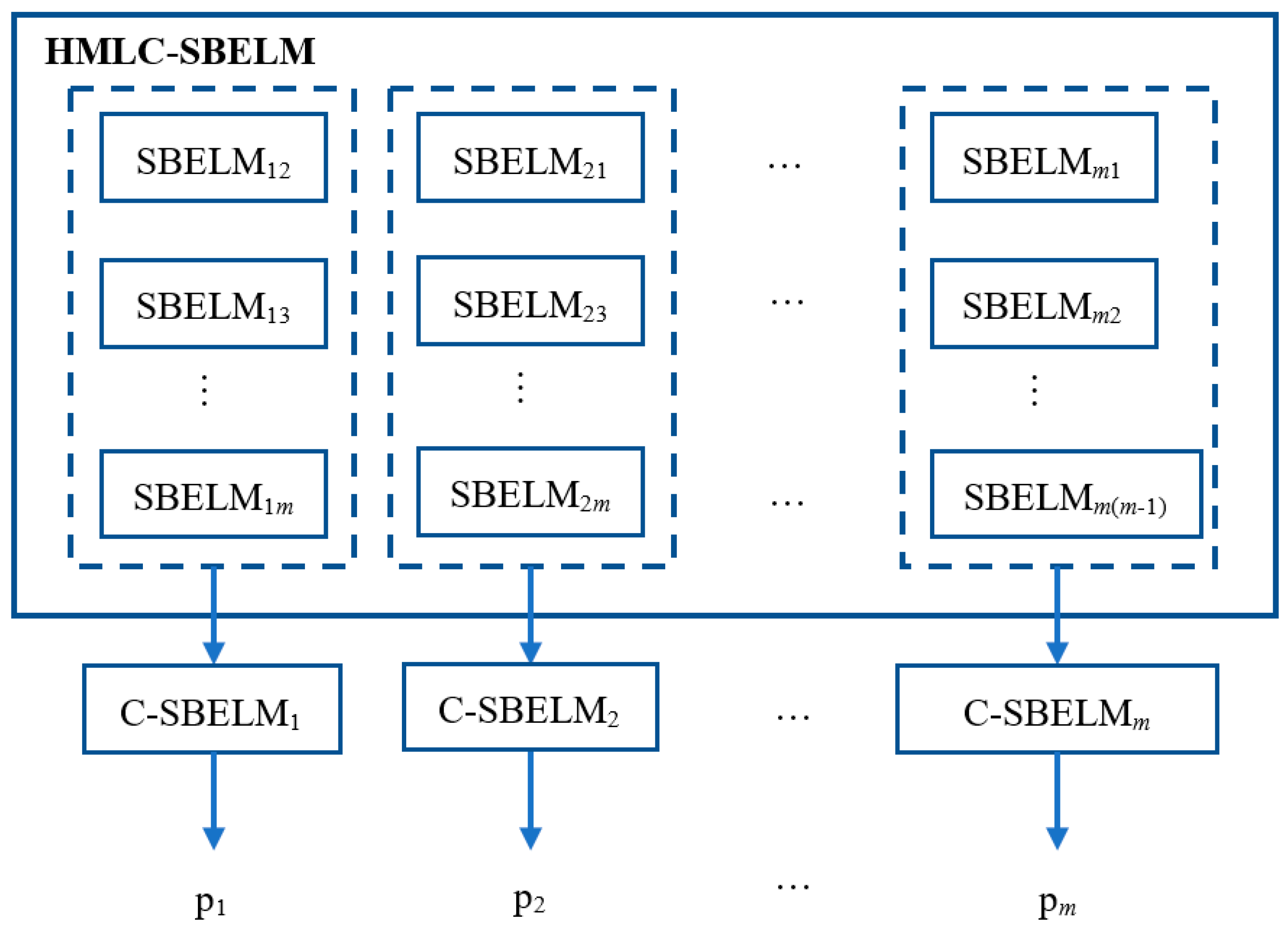
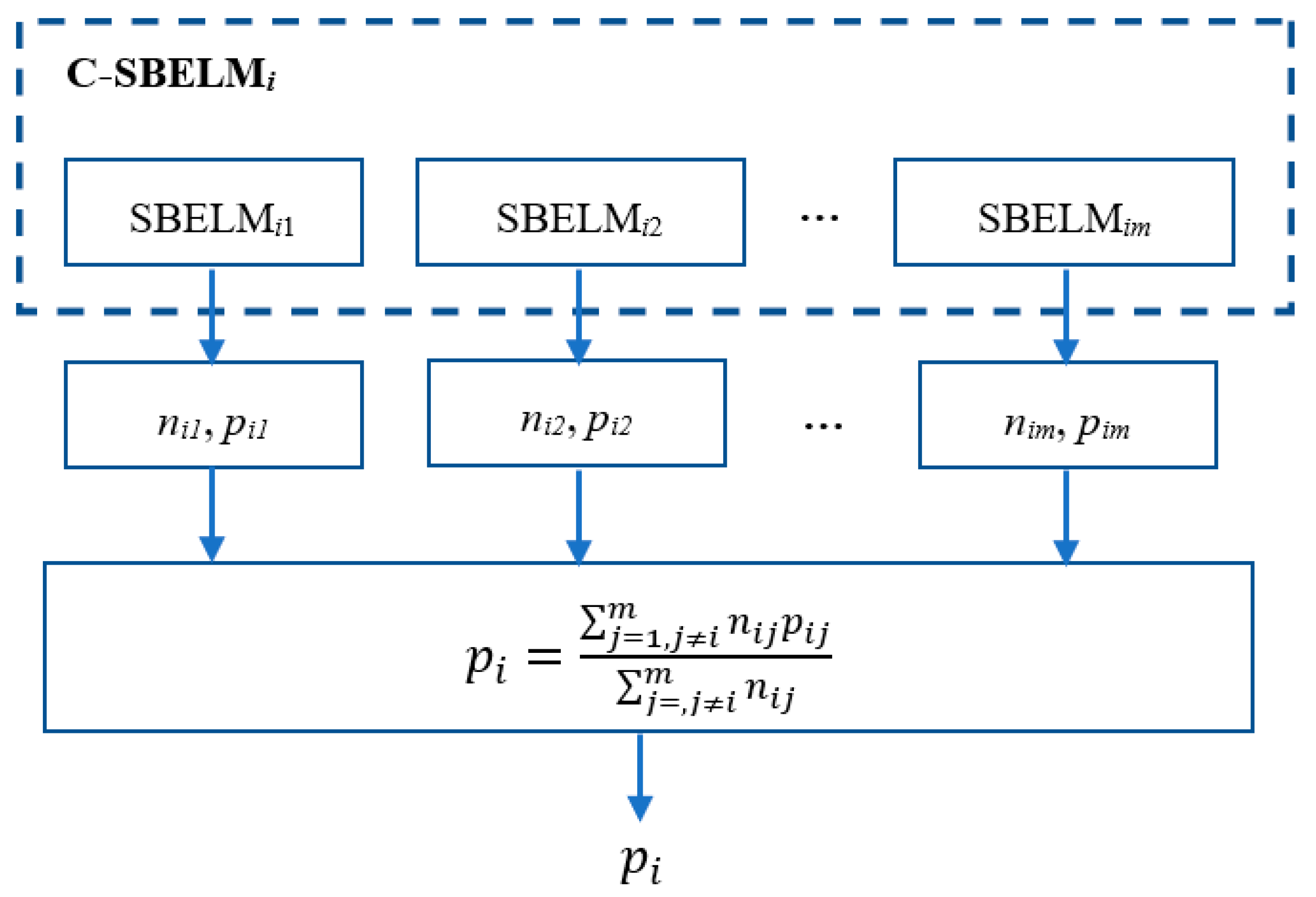
3.3. The Probability Output Fusion of Model Based on HMLC-SBELM

Based on the basic idea of information fusion, we fuse the probabilistic output of each sub-classifier SBELM_ij to acquire the fusion output p_i of each combinational SBELM (C-SBELM), which reflects the occurrence probability of each failure mode. The output matrix of the model is shown as follows:

$$\mathrm{Matrix} =\left[\begin{array}{ccc}{p}_{12}\left(x\right)& \cdots & p_{1m}\left(x\right)\\ ⋮& \ddots & ⋮\\ p_{m1}\left(x\right)& \cdots & p_{m\left(m-1\right)}\left(x\right)\end{array}\right]$$

(18)

The ith row in the matrix is the possibility of associating the ith failure mode for this sample x, namely the output probability of classifier C-SBELM_i. Since more than one failure mode may emerge at the same time and p_i is an independent probability output for a certain sample x, for simultaneous fault diagnosis ${{\displaystyle \sum }}^{ }{p}_i$ is not necessarily equal to 1.

The training set of each single fault mode that is used to train the two-class classifier SBELM_ij may be unbalanced. Considering the positive correlation between the amount of single-failure samples and the corresponding occurrence probability, the sample size of the training set is taken as the weight coefficient of fusion to generate the fusion result:

$$p_i=\frac{{{\displaystyle \sum }}_{j=1,j\ne i}^m{n}_{ij}{p}_{ij}}{{{\displaystyle \sum }}_{j=,j\ne i}^m{n}_{ij}},i =1,2,\dots ,m$$

(19)

in which $n_{ij}$ represents the number of samples with either the ith or the jth fault mode which are used to train classifier SBELM_ij.

The procedure of probability output fusion is shown in Figure 3.

3.4. The Optimization of Threshold Value

For single fault diagnosis, the failure mode with the highest probability of the output probability vector [p₁, p₂, …, p_m] obtained from diagnostic mode is the predicted result. However, for simultaneous fault diagnosis, the number of single failure modes occurring simultaneously is uncertain. Based on this, a suitable discriminative threshold is crucial to acquire multiple failure modes simultaneously occurring according to the output [p₁, p₂, …, p_m].

Usually, many classification algorithms use 0.5 as the universal threshold, and the probability of greater than 0.5 indicates that some fault occurs, otherwise, the failure does not appear [31,32]. Without considering any apriori information, the universal threshold is not appropriate for some specific fields. In particular, the performance of the universal threshold decreases when the training sample size distribution is heterogeneous.

In this paper, in order to generate a suitable threshold for identifying simultaneous failure modes, single failure samples and simultaneous failure samples are utilized. The range of discriminative threshold ${\epsilon }^{\ast }$ is set to (0, 1). By using the optimal discriminative threshold, [p₁, p₂, …, p_m] is converted into final result vector [f₁, f₂, …, f_m]:

$$f_i=\{\begin{array}{c}1 if p_i \ge {\epsilon }^{\ast }\\ 0 if p_i<{\epsilon }^{\ast }\end{array}, i =1,\dots ,m$$

(20)

in which simultaneous fault modes are the corresponding failure mode with the element 1 in the result vector [f₁, f₂, …, f_m]. Based on the global optimization ability and the advantages of small calculation of particle swarm optimization (PSO) [33,34], this paper uses the following formula as the objective function to obtain the optimal value of the decision threshold:

$$\min \left(1-\mathrm{F}\right)$$

(21)

where F represents the F1-measure indicator.

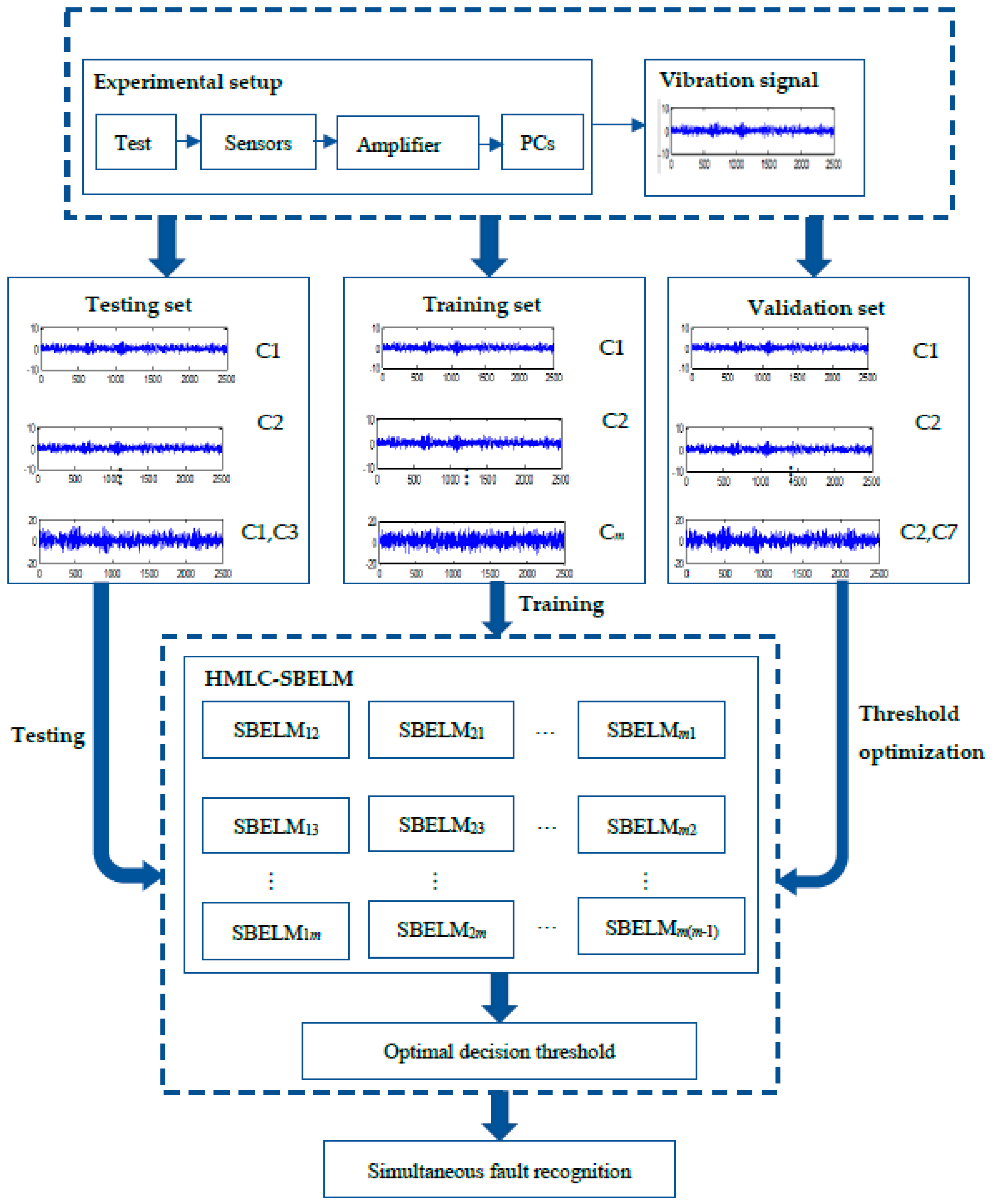
3.5. The Architecture of the Framework Based on HMLC-SBELM

The structure of the proposed diagnostic framework based on HMLC-SBELM is shown in Figure 4.

The steps of the proposed diagnostic framework are summarized below:

(1) Collect a large number of single failure mode samples and a small number of simultaneous failure mode samples from the actual environment. The vast majority of single failure samples are extracted to generate a training set, and the remaining single failure samples and simultaneous failure samples are divided into two subsets to generate the validation set and testing set. All the samples were preprocessed to increase the signal-to-noise ratio and extract typical features.

(2) The diagnostic model training module: use the training set to train the HMLC-SBELM-based model which can efficiently solve the classification problem with multiple classes benefiting from the advantage in a sparse representation based on probability inference.

(3) The optimal threshold determination module: use the validation set and adopt the F1-measure index as the standard measurement of diagnostic accuracy. The particle swarm optimization algorithm is utilized to optimize a suitable discriminative threshold which is critical for simultaneous fault recognition. With the discriminative threshold, the probability output vector of the diagnostic model trained in Step (2) is transformed into the final failure modes.

(4) Performance evaluation module of the diagnostic model: the testing set and the optimal threshold determined in Step (3) is used to evaluate the performance of the diagnostic model.

4. Experiment and Discuss

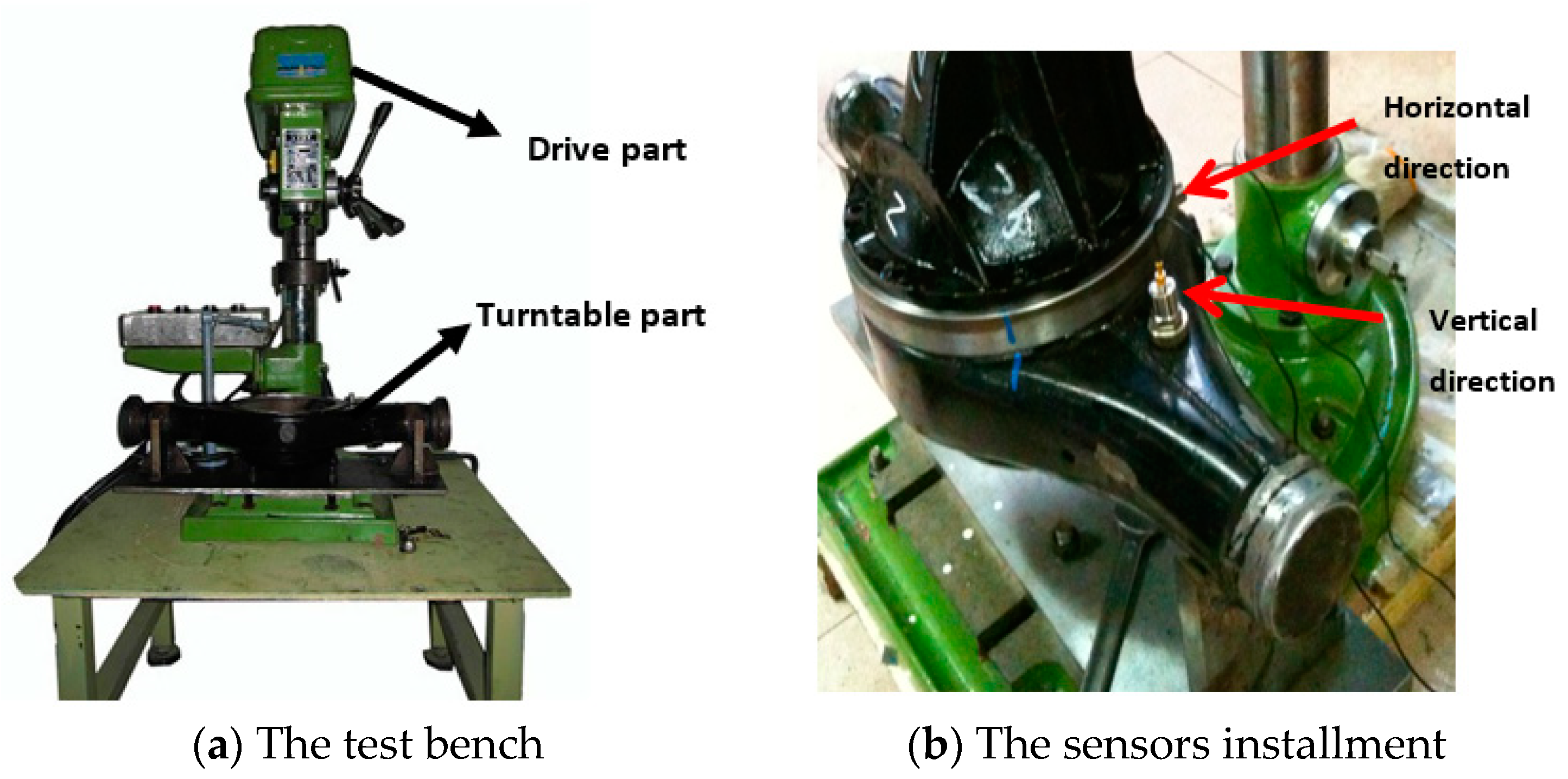
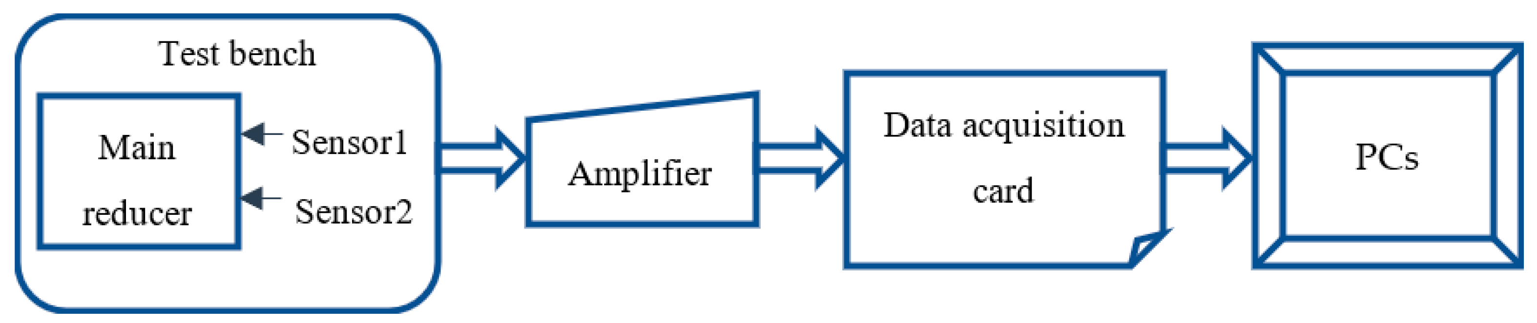
4.1. Experimental Environment and Setup

In this paper, a data acquisition test bench was used to collect the vibration signals in the actual environment. Through destructive experiments, the faulty main reducers with some particular failure modes such as tooth surface knock, tooth surface wear, and tooth surface bonding were obtained to ensure the repeatability of the collected signals. The test bench is shown in Figure 5a, and the sensors installment is shown in Figure 5b. In order to collect the vibration signal during the running of the main reducer more accurately, two acceleration sensors are placed in the lateral direction and the longitudinal direction of the main reducer as shown in Figure 6.

The rotating speed of the test bench is set to 800 rpm (round per minute) at a sampling frequency of 1024 Hz. To ensure that the valuable fault information is not lost during the sampling process, the sampling frequency must be higher than the mesh frequency of the gear pair inside the main reducer. The vibration signals collected within 2 s after the motor begins working and the signals collected within 2 s before the termination of motor operation are discarded. That is, delay 2 s to start the sampling so as to sample in the most stable state of the motor operation.

According to prior knowledge, this paper mainly focuses on the six most common single failure modes of the main reducer. In order to build an intelligent simultaneous fault diagnosis framework of the main reducer, since it is infeasible to simulate all possible simultaneous failure modes, the five most common simultaneous failure modes are selected in this study. The description of several failure modes is in

Table 1. Failure modes description.

Failure Type	Failure No.	Description
Single fault	C1	Normal state
	C2	Gear hard point
	C3	Gear crack
	C4	Gear tooth broken
	C5	Gear burr
	C6	Gear error
	C7	Misalignment
Simultaneous fault	C2, C3	Gear hard point and gear crack
	C3, C6	Gear crack and gear error
	C5, C7	Gear burr and misalignment
	C2, C3, C6	Gear hard point, gear crack and gear error
	C3, C5, C7	Gear crack, gear burr and misalignment

.

Based on the test bench of the main reducer, the collected data contains 500 normal samples, 3000 single failure sample, and 2500 simultaneous failure samples. The assignment of experimental parameters is in

Table 2. Assignment of the experimental dataset.

	Single Failure Samples	Simultaneous Failure Samples	Total
Training set	350 × 7	None	2450
Validation set	100 × 7	400 × 5	2700
Testing set	50 × 7	100 × 5	850
Total	3500	2500	6000

, where the number of sampling points per sample is 2048. All simulation experiments are performed by Matlab 7.0 on a computer with a CPU of 3.4 GHz and 4.0 GB of memory.

4.2. Model Parameter Setup

In this paper, some state-of-the-art methods containing probability neural network (PNN) [35,36], SVM, ELM, and kernel ELM (KELM) [37,38,39] are used to construct diagnostic models for comparison.

To obtain the optimal decision threshold for identifying the various modes, an independent determination threshold set Dthresholding containing both single failure and multiple faults is utilized to optimize an appropriate discriminative threshold ε* within the interval [0, 1] by using PSO [40,41]. The inertial weight of the PSO algorithm which is used to balance the ability of global search and local search is set to 0.9, the learning factors are set to 2, the iteration number is set to 1000, and the population size is 100.

For the diagnostic model based on SVM, the regularization parameter C is set to 1.0, and the sigmoid kernel function is utilized in which the parameter γ is set to 1.0. The diagnostic model based on KELM uses the same parameter sets C and γ with a default value of 1.0. For the diagnostic model based on ELM, the optimal number of hidden nodes is searched in the range of 10 and 300 with the increment of 10.

PNN is a typical probability classifier, and the parameter spread is greatly related to the performance. With a smaller spread value, the function fits smoother and the error becomes larger. Meanwhile, the calculation cost of the network is more, and vice versa.

4.3. Comparative Analysis and Experimental Results

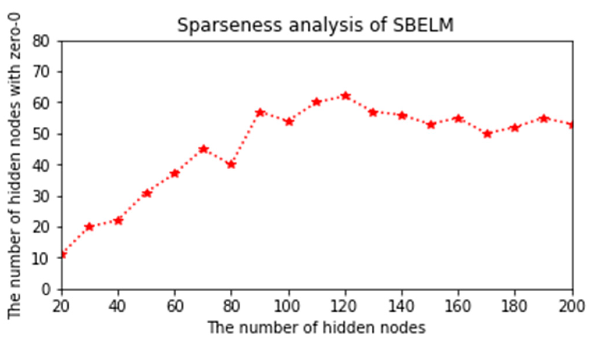
4.3.1. Sparseness Analysis of SBELM

The size of classification models based on SVM and KELM depends on the training set size, and the training time also gradually increases as the training set size gradually rises. However, the size of ELM-based and SBELM-based classification models depends on the hidden layer scale. Therefore, the running efficiency of ELM-based and SBELM-based models is superior to SVM-based and KELM-based models. By using the sparse Bayesian framework to prune the initial hidden layer, SBELM is able to retain a small hidden layer scale with non-zero output weights to express the hidden layer sparsely. Accordingly, the SBELM-based classification model is more compact and concise.

The training set which contains 2450 single-fault samples is utilized to train the SBELM-based classification model. The hidden layer scale is increased with an increment of 10 from 20 to 200 to study the sparse representation rate of the hidden layer nodes.

As shown in Figure 7, the SBELM-based classification model finally retains 53 hidden layer nodes with non-zero weights from 200 initial hidden nodes. The sparse representation rate is nearly 1:4. Meanwhile, when the initially hidden layer scale is greater than 120, the non-zero hidden layer nodes remain on a similar order of magnitude. The results show that in the training phase of the SBELM-based model, the model with 200 initial hidden layer nodes can further realize the sparse representation of the hidden layer.

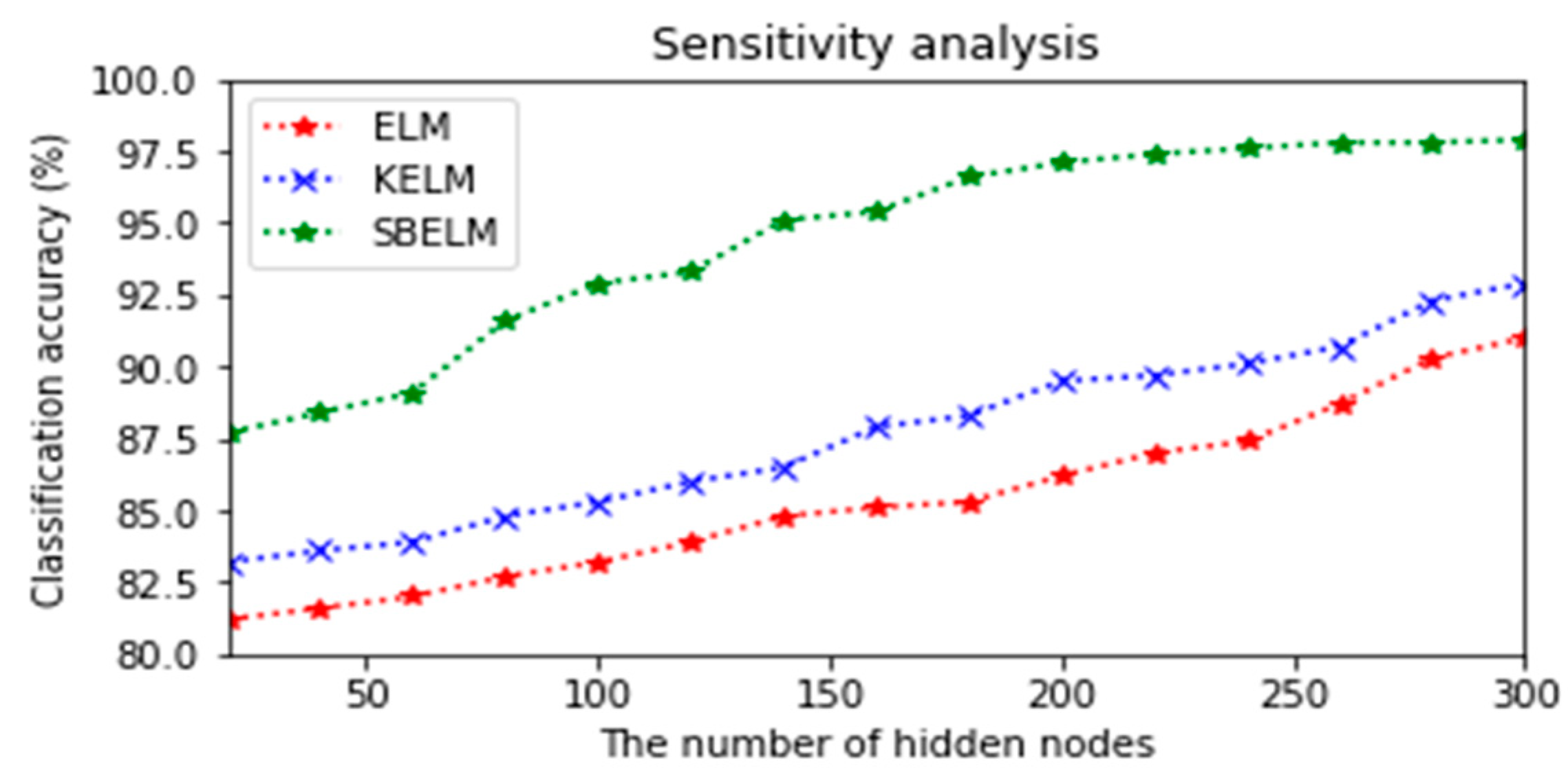
4.3.2. Sensitivity Analysis for the Hidden Layer Scale

By referring to some representative literature, we used 300 as the upper limit of the hidden layer scale, with an increment of 20. With the increase in the hidden layer scale, the optimal classification accuracies of three contrastive classification models are illustrated in Figure 8.

With the enlargement of the hidden layer scale, the average accuracy of classification models based on ELM and KELM changes obviously. The accuracy is relatively low when the hidden layer scale is small. It shows that ELM and KELM are sensitive to the hidden layer scale. To achieve high accuracy, the model must contain a largely hidden layer. Since the size of the ELM-based model is high related to the hidden layer scale, a larger model will cause a relatively long classification time.

The performance of the SBELM-based classification model basically maintains a relatively fixed region, and it is always superior to the ELM-based and KELM-based by nearly 10%. When the number of the hidden layer nodes is in the range of 200–300, the classification accuracy of the SBELM-based model is relatively stable, remaining between 97% and 98%. It indicates that the SBELM-based model is relatively insensitive to the initially hidden layer scale.

The SBELM-based model can also achieve high classification accuracy even with fewer hidden nodes. A small hidden layer scale can greatly decrease the computational cost of training. Based on the above comparison results, the maximum hidden layer size is chosen as 200.

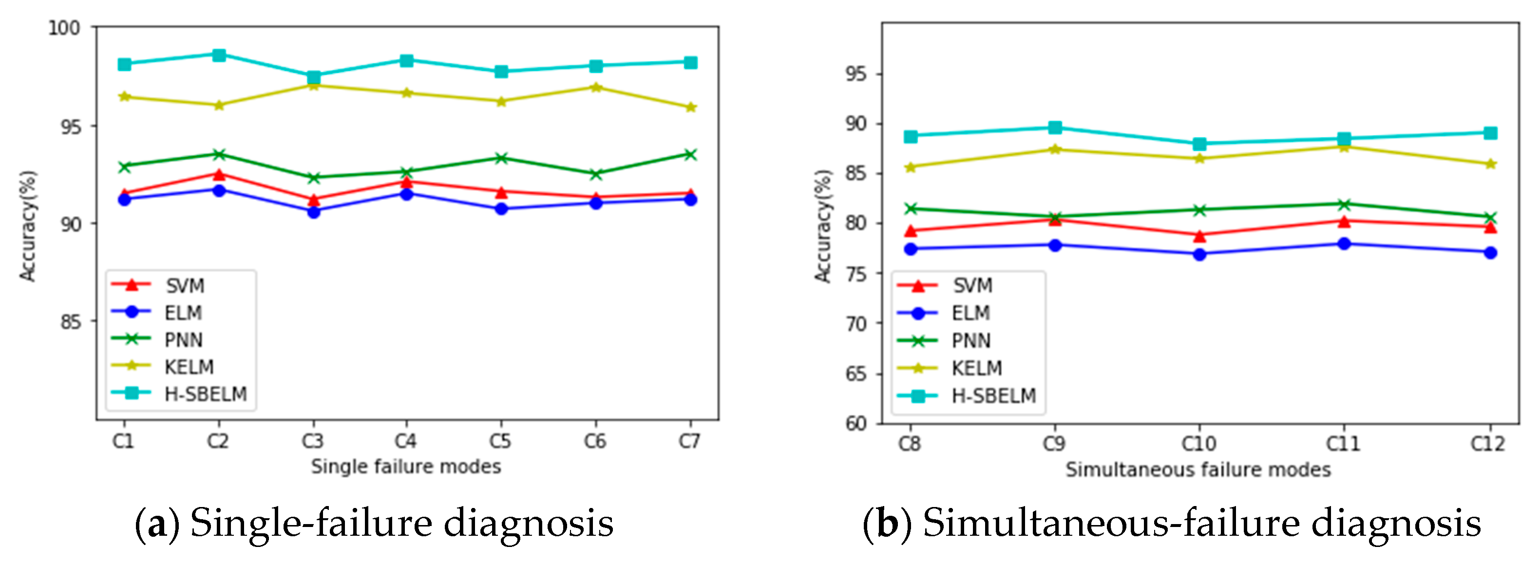
4.3.3. Performance Evaluation of the Diagnostic Framework

(1)

Training of HMLC-SBELM-based model

During the training of the diagnostic model based on HMLC-SBELM, due to the probability output characteristic of SBELM, the diagnostic model outputs a probability vector represented as p = [p₁,…,p_m] in which m is the number of a single fault. The prediction result is the failure mode corresponding to the largest element in the probabilistic output vector = [p₁,…,p₇].

As indicated in

Table 3. The probability output vector of the proposed model.

No.	Actual Category	${\mathit{p}}_1$	${\mathit{p}}_2$	${\mathit{p}}_3$	${\mathit{p}}_4$	${\mathit{p}}_5$	${\mathit{p}}_6$	${\mathit{p}}_7$	Predicted Result
1	1	0.7218	0.0256	0.0672	0.1005	0.1026	0.0052	0.2735	1
2	1	0.7237	0.2096	0.0034	0.1128	0.0007	0.1265	0.1542	1
3	1	0.7623	0.0028	0.1205	0.0005	0.1037	0.0039	0.0126	1
4	1	0.8906	0.2118	0.0087	0.0132	0.0005	0.0458	0.0001	1
5	1	0.7314	0.0075	0.3008	0.0009	0.0386	0.0012	0.0006	1
6	1	0.7209	0.1022	0.1102	0.0026	0.0065	0.0725	0.0214	1
…
2447	7	0.1115	0.0009	0.0077	0.1026	0.0059	0.0437	0.7601	7
2448	7	0.0021	0.0097	0.0382	0.0815	0.1027	0.0829	0.7268	7
2449	7	0.2091	0.0038	0.0006	0.1081	0.0077	0.0021	0.7523	7
2450	7	0.1518	0.0009	0.0738	0.0021	0.1703	0.0977	0.7139	7

, the training accuracy of the diagnostic model based on HMLC-SBELM which is trained by using is 99.5%. Moreover, the values of each element p_i of the probability output vector p are significantly different and relatively scattered. It indicates that the trained diagnostic model has high-performance reliability, and very few samples are misdiagnosed. Through further analysis, it is found that in the probability output vector of the misclassified sample, although the probability value corresponding to the actual category is not the maximum value of the seven elements, it is also ranked relatively high and relatively close to the probability value corresponding to the predicted category.

(2)

Determine the optimal decision threshold for the diagnostic model

To achieve the identification of various different forms of failure modes, using the validation set an optimization algorithm is used to optimize an appropriate discriminative threshold ε* which is in (0, 1). The PSO is utilized to optimize the discriminative threshold by performing 50 trials to obtain the average value of the objective function.

After performing multiple iterations, the optimization of the decision threshold using PSO yields, small objective functions, and the corresponding F_me value is 0.923 which indicates that the model performance is obviously high. In addition, the standard deviation of 50 trials is 1.79 × 10⁻³ which reaches a lower level, indicating that PSO shows a stable performance in the decision threshold optimization problem.

To contrast with the existing machine learning algorithms, the discriminative thresholds of models based on some typical and representative methods are, respectively optimized using PSO. The optimal decision thresholds and corresponding Fme are shown in

Table 4. The optimal decision threshold and F_me.

Contrastive Models	PNN		SVM		ELM		KELM		HMLC-SBELM
	ε*	${\mathit{F}}_{\mathit{m}\mathit{e}}$	ε*	${\mathit{F}}_{\mathit{m}\mathit{e}}$	ε*	${\mathit{F}}_{\mathit{m}\mathit{e}}$	ε*	${\mathit{F}}_{\mathit{m}\mathit{e}}$	ε*	${\mathit{F}}_{\mathit{m}\mathit{e}}$
ε*, $F_{me}$	0.71	0.863	0.68	0.829	0.69	0.857	0.69	0.903	0.71	0.923

. As shown in Table 4, the optimal decision threshold of the diagnostic model based on HMLC-SBELM is 0.71. Moreover, the classification accuracy index Fme of the HMLC-SBELM-based model is 0.923, which is superior to other contrastive models with an increase of about 3% to 10%.

(3)

Performance evaluation of the diagnostic model

The performance of various diagnostic models is evaluated by using the testing set Dtesting which contains both single and simultaneous fault samples. The comparison results are listed in

Table 5. The contrastive results of diagnostic models.

Various Models	Multi-Label Classification Strategy	Accuracy (%)
		Single Failures	Simultaneous Failures	Overall Results
PNN	One-to-all	88.45 (±1.52)	78.15 (±1.63)	82.79 (±1.49)
	HMLC strategy	92.88 (±1.31)	81.26 (±1.49)	86.37 (±1.72)
SVM	One-to-all	90.12 (±1.25)	76.23 (±1.75)	81.94 (±1.44)
	HMLC strategy	91.69 (±1.18)	79.81 (±1.52)	84.52 (±1.29)
ELM	One-to-all	85.61 (±1.46)	74.08 (±1.91)	82.91 (±1.55)
	HMLC strategy	91.19 (±1.37)	77.35 (±1.68)	85.44 (±1.59)
KELM	One-to-all	93.26 (±1.54)	83.62 (±1.62)	89.17 (±1.77)
	HMLC strategy	96.38 (±1.71)	86.31 (±1.43)	91.93 (±1.65)
HMLC-SBELM	One-to-all	93.62 (±1.05)	85.38 (±1.45)	88.24 (±1.23)
	HMLC strategy	98.03 (±0.96)	88.71 (±1.01)	94.43 (±1.14)

and shown in Figure 9 in which H-SBELM represents the HMLC-SBELM-based model.

As indicated in Figure 9, among the above-mentioned five diagnostic models, the HMLC-SBELM-based diagnostic model outperforms other models in recognizing single-fault modes and simultaneous failure modes. Unlike other models by employing regression and fitting to solve the problem, the SBELM-based model improves the generalization performance by the probability distribution estimation. For seven single failure modes and five simultaneous failure modes, the average testing accuracy of HMLC-SBELM reach 98.03% and 88.71%. The diagnostic accuracy is improved by 5% to 15% over several other diagnostic models.

In the proposed HMLC-SBELM-based model, the HMLC strategy is closely related to the improvement of performance. By comparing the diagnostic accuracy of the above five diagnostic models with the HMLC strategy and traditional one-to-all multi-class classification strategy, the effectiveness of the HMLC strategy is validated and the results are listed in Table 5.

As illustrated in Table 5, for the same diagnostic model, the classification accuracy of diagnostic models with the HMLC strategy is 2% to 6% higher than that of models with a one-to-all strategy. The main reasons are that the hierarchical pairing framework proposed in this paper fully considers the correlation between multiple single failure modes when diagnosing multiple faults. For the diagnostic model with a one-to-all strategy, inseparable regions (indecision region) are easy to appear between different failure categories, and the existence of inseparable regions is prone to cause fault misclassification in simultaneous fault diagnosis and further reduce the diagnostic accuracy.

By longitudinally comparing the average classification accuracy of these diagnostic models, models based on SVM are lower than models based on ELM and KELM. The main reason is that the ELM-based model searches for the optimal solution for classification in a large feature space, while the SVM-based model tries to search for the solution in a linear plane, which enables the ELM-based model to obtain better classification solutions than SVM.

The accuracy of the KELM-based diagnostic model with a one-to-all strategy is 93.26% which is higher than the proposed model with a one-to-all strategy in the single fault diagnosis. It can be concluded that KELM inherits the characteristics of high generalization from ELM. Moreover, KELM has its own advantages, that is, hidden-layer nonlinear feature maps are represented as a kernel function.

(4)

Admissibility of simultaneous fault diagnosis results

As listed in Table 5, the diagnostic accuracy of the contrastive models does not exceed 90%, meaning that 10% of the simultaneous failure samples are misclassified. Due to the characteristics of the probability output of the proposed model based on HMLC-SBELM, before the final diagnosis is obtained based on the optimal discriminative threshold, the model will output a probability output vector in which each element of the vector represents the probability of a certain single failure mode.

For simultaneous fault diagnosis, a partial matching between the diagnostic results with actual multiple failures is also valuable. If the occurred single failure mode is still contained in the diagnostic result vector of a misclassified simultaneous-failure sample, it indicates that the result is also acceptable to some extent.

To evaluate the admissibility of simultaneous fault diagnosis model, focusing on 500 simultaneous failure samples in the testing set, analyze the output vector of 56 misclassified samples. A misclassified sample with gear hard point failure (C2) and gear crack failure (C3) is taken as an example, the probatilistic output vector is [0.013, 0.825, 0.629, 0.004, 0.001, 0.033, 0.108]. By using the discriminative threshold 0.71, the result vector is [0, 0, 0, 0, 0, 0, 1] and the sample is recognized as single fault C2. Although the decision result is wrong, it is not difficult to find out that the probability output value of C3 is 0.629, which is still very close to the decision threshold. On the other hand, the decision result still correctly identifies one of the actually emerged single-failure modes. The analysis illustrates that the proposed model based on HMLC-SBELM is highly acceptable and can provide superior technical support and contribution of the practical simultaneous fault diagnosis.

(5)

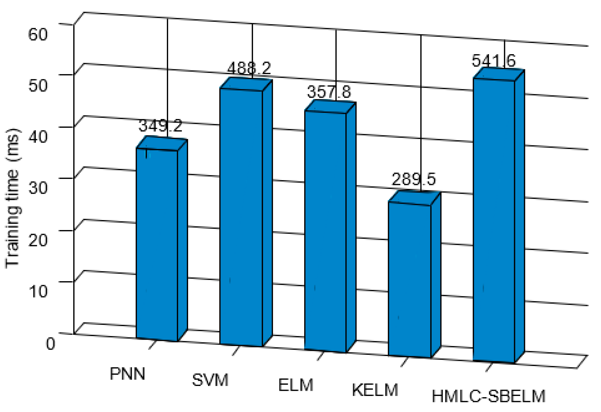
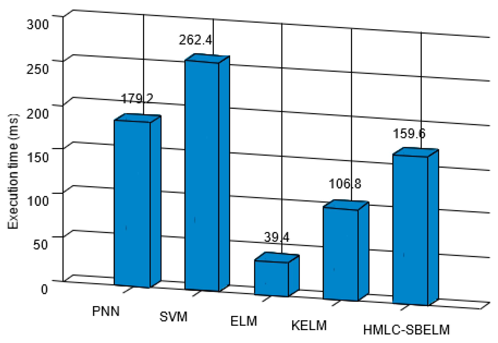
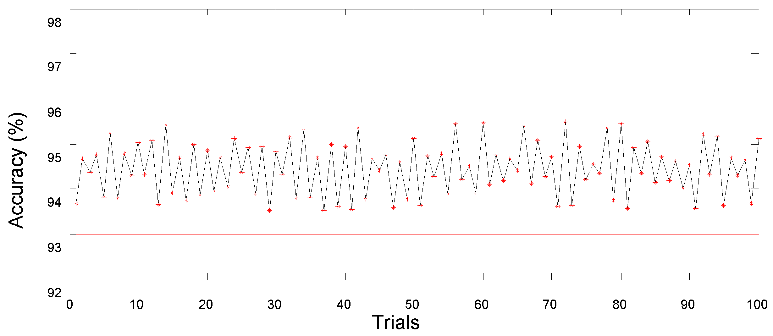
Analysis of efficiency and stability

In addition to the high diagnostic accuracy, the execution time is another key criterion for measuring the model’s performance. Therefore, the training time and execution time of the testing set are compared between these five models to measure the model’s efficiency. Thet results are shown in Figure 10 and Figure 11.

As shown in Figure 10, the training time of the KELM-based model is the shortest, while the training time of the HMLC-SBELM-based model takes the longest training time. The main reason is that the HMLC-SBELM-based model approximates the output weight in an iterative way, and the iterative process is relatively time-consuming. In contrast, SVM, ELM, and KELM all solve the output weights directly by analytical computation, so the training time is relatively short. Although the HMLC-SBELM-based model is time-consuming in the training stage, the training time remains around 0.5 s, which is completely acceptable in practice.

The time cost of classifying the testing set which is composed of 800 samples is shown in Figure 11. It indicates that the execution time of the HMLC-SBELM-based model is only 39.4 ms, which is nearly 4 times faster than other models. In practice, the execution time of a single sample is extremely small. The extremely fast execution speed of the HMLC-SBELM-based model is chiefly due to the minimum hidden layer scale obtained through the sparse Bayesian framework.

To further measure the stability and validity of the proposed intelligent diagnostic model based on HMLC-SBELM, the model was run for 100 trials. In each trial, the entire data set is shuffled and reassigned to obtain a diverse training set, v set, and testing set. The diagnostic accuracies of 100 trials are shown in Figure 12.

As illustrated in Figure 12, the diagnostic results of 100 trials are relatively stable which are between 93% and 96% with no obvious fluctuations. It indicates that the proposed intelligent HMLC-SBELM-based model based on is a high-precision and efficient diagnostic model, which can effectively solve the simultaneous fault mode diagnosis.

5. Conclusions

In this paper, a modified hierarchical multi-label classification (HMLC) strategy is proposed to solve the classification problem with multiple categories and multiple labels. The novel strategy is combined with sparse Bayesian ELM (SBELM) to construct a probabilistic classifier that outputs a probability vector. A series of classifiers based on SBELM is hierarchically organized and generate a model based on HMLC-SBELM. According to the characteristics of the HMLC strategy, the HMLC-SBELM-based model is trained using a large number of single failure samples which are easily obtained. Inadequate simultaneous failure samples are used to optimize the discrimination threshold which is effective for simultaneous fault diagnosis and to test the model performance.

The contributions of this paper are organized into three points: (1) The training of the diagnostic model does not need simultaneous failure samples which can effectively solve the bottleneck of collecting abundant simultaneous failure samples in practical engineering. (2) The novel HMLC strategy can achieve classification tasks with multiple labels which can preferably extract the correlation between various pairs of single faults. (3) Based on the advantages of SBELM, the proposed model can mine the probabilistic correspondence between collected representational data and simultaneous failure modes.

The proposed HMLC-SBELM-based model is applied to simultaneous fault diagnosis for automobile main reducer and plays a huge role in the intelligent diagnosis of recognizing both single fault and simultaneous fault to achieve superior performance. The research is based on vibration signal which is the most common type of data source in the mechanical engineering field. The proposed strategy and model can also be migrated or transformed into other mechanical equipment troubleshooting areas.

In the future, our research will focus on the field of fault recognition based on unsupervised learning to better adapt to the characteristics of collecting data labeling difficulties. Additionally, early warning of failures and remaining life prediction is also a research direction worth attention.

References

1. Yao, L.-J.; Ding, J.-X. An On-line Vibration Monitoring System for Final Drive of Automobile. Noise Vib. Control. 2007, 27, 54–57. [Google Scholar]
2. Ye, Q.; Liu, S.; Liu, C. A Deep Learning Model for Fault Diagnosis with a Deep Neural Network and Feature Fusion on Multi-Channel Sensory Signals. Sensors 2020, 20, 4300. [Google Scholar] [CrossRef] [PubMed]
3. Lee, J.; Wu, F.J.; Zhao, W.; Ghaffari, M.; Liao, L.X.; Siegel, D. Prognostics and health management design for rotary machinery systems: Reviews, methodology and applications. Mech. Syst. Signal Process. 2014, 42, 314–334. [Google Scholar] [CrossRef]
4. Ye, Q.; Liu, C. A Multichannel Data Fusion Method Based on Multiple Deep Belief Networks for Intelligent Fault Diagnosis of Main Reducer. Symmetry 2020, 12, 483. [Google Scholar] [CrossRef]
5. Qi, Y.; Shen, C.; Wang, D.; Shi, J.; Jiang, X.; Zhu, Z. Stacked sparse autoencoder-based deep network for fault diagnosis of rotating machinery. IEEE Access 2017, 5, 15066–15079. [Google Scholar] [CrossRef]
6. Liu, G.; Bao, H.; Han, B. A stacked autoencoder-based deep neural network for achieving gearbox fault diagnosis. Math. Probl. Eng. 2018, 2018, 5105709. [Google Scholar] [CrossRef]
7. Ye, Q.; Liu, C. An Unsupervised Deep Feature Learning Model Based on Parallel Convolutional Autoencoder for Intelligent Fault Diagnosis of Main Reducer. Comput. Intell. Neurosci. 2021, 2021, 8922656. [Google Scholar] [CrossRef]
8. Liu, R.; Yang, B.; Zio, E.; Chen, X. Artificial intelligence for fault diagnosis of rotating machinery: A review. Mech. Syst. Signal Process. 2018, 108, 33–47. [Google Scholar] [CrossRef]
9. Wu, Y.; Jin, W.; Li, Y.; Wang, D. A novel method for simultaneous-fault diagnosis based on between-class learning. Measurement 2021, 172, 108839. [Google Scholar] [CrossRef]
10. Liang, P.; Deng, C. Single and simultaneous fault diagnosis of gearbox via a semi-supervised and high-accuracy adversarial learning framework. Knowl.-Based Syst. 2020, 198, 105895. [Google Scholar] [CrossRef]
11. Tan, Y.; Zhang, J.; Tian, H.; Jiang, D.; Guo, L.; Wang, G.; Lin, Y. Multi-label classification for simultaneous fault diagnosis of marine machinery: A comparative study. Ocean. Eng. 2021, 239, 109723. [Google Scholar] [CrossRef]
12. Zare, S.; Ayati, M. Simultaneous fault diagnosis of wind turbine using multichannel convolutional neural networks. ISA Trans. 2021, 108, 230–239. [Google Scholar] [CrossRef] [PubMed]
13. Guangbin, H.; Zhu, Q.; Siew, C.K. Extreme learning machine theory and applications. Neurocomputing 2006, 70, 489–501. [Google Scholar]
14. Cambria, E. Extreme Learning Machines. IEEE Trans. Cybern. 2013, 28, 30–59. [Google Scholar]
15. Zhang, Y.; Wang, Y.; Zhou, G.; Jin, J.; Wang, B.; Wang, X.; Cichocki, A. Multi-kernel extreme learning machine for EEG classification in brain-computer interfaces. Expert Syst. Appl. 2018, 96, 302–310. [Google Scholar] [CrossRef]
16. Huang, G.; Ding, X.; Zhou, H. Optimization method based extreme learning machine for classification. Neurocomputing 2010, 74, 155–163. [Google Scholar] [CrossRef]
17. Wong, P.K.; Yang, Z.; Vong, C.M.; Zhong, J. Real-time diagnosis fault diagnosis for gas turbine generator systems using extreme learning machine. Neurocomputing 2014, 128, 249–257. [Google Scholar] [CrossRef]
18. Tian, Y.; Ma, J.; Lu, C.; Wang, Z. Rolling bearing fault diagnosis under variable conditions using LMD-SVD and extreme learning machine. Mech. Mach. Theory 2015, 90, 175–186. [Google Scholar] [CrossRef]
19. Song, Y.; Crowcroft, J.; Zhang, J. Automatic epileptic seizure detection in EEGs based on optimized sample entropy and extreme learning machine. J. Neurosci. Methods 2012, 210, 132–146. [Google Scholar] [CrossRef]
20. Huang, G.B.; Zhou, H.; Ding, X.; Zhang, R. Extreme learning machine for regression and multiclass classification. IEEE Trans. Syst. Man Cybern. B: Cybern. 2012, 42, 513–529. [Google Scholar] [CrossRef]
21. Emilio, S.O.; Juan, G.S.; Martin, J.D.; Vila-Frances, J.; Martinez, M.; Magdalena, J.R.; Serrano, A.J. BELM: Bayesian extreme learning machine. IEEE Trans. Neural Netw. 2011, 22, 505–509. [Google Scholar]
22. Zhang, Y.; Jin, J.; Wang, X.; Wang, Y. Motor imagery EEG classification via Bayesian extreme learning machine. In Proceedings of the IEEE Sixth International Conference on Information Science and Technology (ICIST 2016), Dalian, China, 6–8 May 2016; pp. 27–30. [Google Scholar]
23. Udmale, S.S.; Singh, S.K. Application of spectral kurtosis and improved extreme learning machine for bearing fault classification. IEEE Trans. Instrum. Meas. 2019, 68, 4222–4233. [Google Scholar] [CrossRef]
24. Luo, J.; Vong, C.M.; Wong, P.K. Sparse Bayesian extreme learning machine for multi- classification. IEEE Trans. Neural Netw. Learn. Syst. 2014, 25, 836–842. [Google Scholar] [PubMed]
25. Suresh, S.; Saraswathi, S.; Sundararajan, N. Performance enhancement of extreme learning machine for multi-category sparse data classification problems. Eng. Appl. Artif. Intell. 2010, 23, 1149–1157. [Google Scholar] [CrossRef]
26. Chen, S.; Gao, L.; Liao, G. MBAN-MLC: A multi-label classification method and its application in automating fault diagnosis. Int. J. Internet Manuf. Serv. 2018, 5, 350–364. [Google Scholar] [CrossRef]
27. Chen, W.-J.; Shao, Y.-H.; Li, C.-N.; Deng, N.-Y. MLTSVM: A novel twin support vector machine to multi-label learning. Pattern Recogn. 2016, 52, 61–74. [Google Scholar] [CrossRef]
28. Boutell, M.R.; Luo, J.; Shen, X.; Brown, C.M. Learning multi-label scene classification. Pattern Recogn. 2004, 37, 1757–1771. [Google Scholar] [CrossRef]
29. Ning, K.; Liu, M.; Dong, M.; Wu, C.; Wu, Z. Two efficient twin ELM methods with prediction interval. IEEE Trans. Neural Netw. Learn. Syst. 2015, 26, 2058–2071. [Google Scholar] [CrossRef]
30. Zhao, R.; Mao, K. Semi-random projection for dimensionality reduction and extreme learning machine in high-dimensional space. IEEE Comput. Intell. Mag. 2015, 10, 30–41. [Google Scholar] [CrossRef]
31. Yu, H.; Mu, C.; Sun, C.; Yang, W.; Yang, X.; Zuo, X. Support vector machine-based optimized decision threshold adjustment strategy for classifying imbalanced data. Knowl.-Based Syst. 2015, 76, 67–78. [Google Scholar] [CrossRef]
32. Lipton, Z.C.; Elkan, C.; Naryanaswamy, B. Optimal thresholding of classifiers to maximize F1 measure. Mach. Learn. Knowl. Discov. Databases 2014, 8725, 225–239. [Google Scholar] [PubMed]
33. Haas, D.; Painter, F.D.; Wilkinson, M. Root-cause analysis of simultaneous faults on an offshore FPSO vessel. IEEE Trans. Ind. Appl. 2014, 50, 1543–1551. [Google Scholar] [CrossRef]
34. Barbieri, R.; Barbieri, N.; De Lima, K.F. Some applications of PSO for optimization of acoustic filters. Appl. Acoust. 2015, 89, 62–70. [Google Scholar] [CrossRef]
35. Ali, J.B.; Saidi, L.; Mouelhi, A.; Chebel-Morello, B.; Fnaiech, F. Linear feature selection and classification using PNN and SFAM neural networks for a nearly online diagnosis of bearing naturally progressing degradations. Eng. Appl. Artif. Intell. 2015, 42, 67–81. [Google Scholar]
36. Chen, X.; Zhou, J.; Xiao, H.; Wang, E.; Xiao, J.; Zhang, H. Fault diagnosis based on comprehensive geometric characteristic and probability neural network. Appl. Math. Comput. 2014, 230, 542–554. [Google Scholar] [CrossRef]
37. Huang, G.B. An insight into extreme learning machines: Random neurons, random features and kernels. Cogn. Comput. 2014, 6, 376–390. [Google Scholar] [CrossRef]
38. Iosifidis, A.; Tefas, A.; Pitas, I. On the kernel extreme learning machine classifier. Pattern Recognit. Lett. 2015, 54, 11–17. [Google Scholar] [CrossRef]
39. Zhang, Y.; Wang, Y.; Jin, J.; Wang, X. Sparse Bayesian learning for obtaining sparsity of EEG frequency bands based feature vectors in motor imagery classification. Int. J. Neural Syst. 2017, 27, 1650032. [Google Scholar] [CrossRef]
40. Liu, Z.; Zhang, L. A review of failure modes, condition monitoring and fault diagnosis methods for large-scale wind turbine bearings. Measurement 2020, 149, 107002. [Google Scholar] [CrossRef]
41. Lei, Y.; Yang, B.; Jiang, X.; Jia, F.; Li, N.; Nandi, A.K. Applications of machine learning to machine fault diagnosis: A review and roadmap. Mech. Syst. Signal Process. 2020, 138, 106587. [Google Scholar] [CrossRef]
Figure 1. The structure of hierarchical multi-label classification strategy.
Applsci 13 02376 g001
Figure 2. The architecture of model-based on HMLC-SBELM.
Applsci 13 02376 g002
Figure 3. The procedure of probability output fusion.
Applsci 13 02376 g003
Figure 4. The proposed simultaneous fault diagnostic framework.
Applsci 13 02376 g004
Figure 5. The test bench.
Applsci 13 02376 g005
Figure 6. The process of data acquisition.
Applsci 13 02376 g006
Figure 7. Number of non-zero-weight hidden nodes of the SBELM-based model.
Applsci 13 02376 g007
Figure 8. Sensitivity analysis.
Applsci 13 02376 g008
Figure 9. Comparison of fault diagnostic result.
Applsci 13 02376 g009
Figure 10. Comparison of the training times.
Applsci 13 02376 g010
Figure 11. Comparison of the execution time.
Applsci 13 02376 g011
Figure 12. The results of 100 trials.
Applsci 13 02376 g012