Feature Extraction of Bearing Weak Fault Based on Sparse Coding Theory and Adaptive EWT

Abstract

In industry, early fault signals of rolling bearings are submerged in strong background noise, causing a low signal-to-noise ratio (SNR) and difficult diagnosis. This paper proposes a fault feature extraction method based on an optimized Laplacian wavelet dictionary (LWD) and the feature symbol search (FSS) algorithm to extract early fault characteristic frequencies of bearings under low SNR. As the morphological parameters of the Laplace wavelet dictionary and sparse coefficients are not easy to obtain, this method uses the adaptive empirical wavelet transform (AEWT) to determine the morphological parameters of the Laplace wavelet. Firstly, AEWT is applied to obtain the different frequency components, and the combination index is utilized for optimal component selection. Then, the morphological parameters of LWD are determined by AEWT processing, by which the overcomplete dictionary that best matches the signal can be obtained. Finally, the optimal sparse representation of the component signal in the dictionary is calculated by FSS, which helps to achieve sparse denoising and enhance the impact features. The effectiveness of the method is verified by simulation. The effectiveness and advantages of LWDFSS-AEWT are verified by experiment in comparison with methods such as fast spectral kurtosis (FSK), correlation filtering (CF), shift-invariant sparse coding (SISC), base pursuit denoising (BPDN) and wavelet packet transform Kurtogram (WPT Kurtogram).

1. Introduction

Rolling bearings are crucial but easily damaged components in rotating machinery. Statistics show that more than 30% of mechanical failures are related to bearings in rotating machinery, and the operating status of bearings directly determines whether the equipment can run normally. At present, the most effective and commonly used method of bearing fault diagnosis is vibration analysis. However, in practice, the low SNR and non-stationary nature of early fault vibration signals mean that it is hard to extract fault characteristic information from noise interference signals. How to analyze and process vibration data to obtain fault characteristic information is the main difficulty [1]. Therefore, it is necessary to develop effective signal-processing methods to achieve accurate fault detection. The sparse theory was proposed by Olshausen and Field [2], and has been continuously developed and deepened to the point where it is a subject of intense study in image and signal processing [3,4,5,6,7], and compressed sensing [8]. The sparse representation of signals aims to find the sparsest expression in the redundant atomic dictionary, using the least number of atoms to represent the signal to capture and express the essence of the signal. Du et al. [9] proposed a method to construct different redundant dictionaries according to the different impact morphological characteristics of gear and bearing faults. The method realized the separation of composite faults from gears and bearings utilizing sparse representation. Kong et al. [10] developed an adaptive matching pursuit algorithm to denoise the original signal and then utilized the fast spectrum correlation method to identify the fault category. A framework of sparse representation classification for fault diagnosis in planetary bearings has also been developed [11]. Li et al. [12] adopted the improved parametric of empirical wavelet transforms (EWT) and adaptive sparse coding shrinkage de-noising to carry out adaptive sparse de-noising for the signal of a fault bearing, which is beneficial in increasing the strong pulse features of the fault. He et al. [13] constructed an overcomplete atomic library using the shock function of the second-order bearing damping that was able to identify the natural frequency through the correlation filtering method, and reduce the redundancy of the dictionary. The bearing fault signals were matched by the matching pursuit method improving the efficiency and accuracy of signal reconstruction under low SNR. Tang et al. [14] utilized SISC to achieve feature extraction of early weak faults, verified by vibration signals of bearings and gears and achieved good results. Zhou et al. [15] proposed an algorithm based on the FSS and attenuated cosine dictionary to diagnose bearing weak faults, and compared their method with methods such as BPDN and WPT.

EWT was first proposed by Gilles [16]. Its main idea is to extract the closely supported amplitude and frequency modulation components. Adaptive signal decomposition is then achieved by dividing the Fourier spectrum and constructing a series of orthogonal wavelet filter banks. Chegini et al. [17] combined EWT and an improved threshold function method to reduce the noise of a vibration signal, which was helpful in detecting bearing early faults by signal reconstruction. Chen et al. [1] denoised the vibration signal of a wind turbine generator bearing using a wavelet spatial adjacency coefficient of a data-driven threshold. They then utilized EWT to diagnose weak and composite faults of the bearing. Song et al. [18] presented a combination algorithm based on the Pearson correlation coefficient to correct the over-decomposing tendency of EWT. Cao et al. [19] improved EWT and then applied their improved EWT to fault diagnosis of a train-wheel hub bearing. Jiang et al. [20] proposed a method base on EWT and duffing oscillator to diagnose bearing compound faults and proved the application performance of EWT is better than EMD series methods.

By analyzing the dictionary to generate the overcomplete dictionary required by the sparse algorithm, it is usually necessary to determine the optimization range or exact value of the relevant parameter. In this paper, a sparse dictionary is constructed using a Laplace wavelet, the morphological parameters of which have been a subject of intense research interest. For traditional deterministic morphological parameters methods such as correlation filtering, it is impossible to obtain the damping ratio and resonance frequency parameters when processing low SNR signals. At the same time, if the parameter optimization range is too large, the scale of the dictionary will be extremely large, which can result in extremely low computing efficiency. It can be seen that the superiority of EWT is demonstrated through the analysis of related methods. However, EWT also has challenges, such as over-decomposition inhibition and optimal component selection. Therefore, a feature extraction method of bearing weak faults based on sparse coding theory and adaptive EWT is proposed in this paper. Firstly, the sparse coding theory is briefly described, and the parameter determination method of a Laplace wavelet dictionary combined with the EWT method is provided. Then, the AEWT based on a scale space method is briefly described, and the component selection method is given. Next, the algorithm flow is presented, and the simulation signal and bearing life test data are analyzed. Finally, the proposed method is compared with FSK, CF, SISC based on a learning dictionary, BPDN based on a wavelet packet and the WPT Kurtogram. The results of this comparison verify the superiority of the proposed method.

2. Sparse Coding Algorithm Based on Optimized LWD and FSS

2.1. Shift Invariant Sparse Coding

SISC considers that the same atom (also known as the basis function) through any time shift can express every identical event in the signal. It is very suitable for the effective characterization of periodic feature components in vibration signals. Assuming that the input signal $y_{{}^{\left(i\right)}}\in R^p,i=1,\cdots ,m$, $LD=\left\{\mathrm{l}{d}_{{}^{\left(1\right)}},\mathrm{l}{d}_{{}^{{}^{\left(2\right)}}},\cdots ,\mathrm{l}{d}_{{}^{\left(n\right)}}\right\}$ is a redundant dictionary, and $s={\left\{s_{{}^{\left(1\right)}},s_{{}^{\left(2\right)}},\cdots s_{{}^{\left(\mathrm{n}\right)}},\right\}}^T$ is the sparse coefficient, respectively, then $y_{{}^{\left(i\right)}}$ can be expressed by a time-shifting atom $d_{{}^{\left(j\right)}}\in R^q,j=1,\cdots ,n$ as:

$$y_{{}^{\left(i\right)}}=LDs+{\epsilon }_{{}^{{}_{\left(i\right)}}}={\displaystyle \sum _j^{}\mathrm{l}{d}_{{}^{\left(j\right)}}\ast s_{{}^{\left(i,j\right)}}}+{\epsilon }_{{}^{\left(i\right)}}$$

(1)

where “$\ast$” is the convolution operation, which is used to represent that each atom can move anywhere in the time domain, $s_{{}^{\left(i,j\right)}}\in R^{p-q+1}$ is the sparse coefficient, and ${\epsilon }_{{}^{\left(i\right)}}\in R^p$ is additive random noise. Here, the dimension of atom $d_{{}^{\left(j\right)}}\in R^q$ can be lower than that of the input signal. Assuming that $\beta$ is the sparsity penalty parameter used to control the sparsity degree and c is an iteration error threshold, then the objective function is defined as:

$$\begin{array}{c}\begin{array}{cc}\underset{d,s}{\min }& {{\displaystyle \sum _{i=1}^m‖y_{{}^{\left(i\right)}}-{\displaystyle \sum _{j=1}^{n}l{d}_{{}^{\left(j\right)}}\ast s_{{}^{\left(i,j\right)}}}‖}}_2^2+\beta {\displaystyle \sum _{i,j}{‖s_{{}^{\left(i,j\right)}}‖}_1}\end{array}\\ {\begin{array}{cc}\begin{array}{ccc}& & \end{array}s.t.& ‖l{d}_{{}^{\left(j\right)}}‖\end{array}}_2^2\le c,1\le j\le n\end{array}$$

(2)

2.2. Solving Sparse Coefficient Based on FSS

According to Equation (2), the objective function may not be a convex optimization problem about the atomic dictionary D and the coefficient S at the same time, so it cannot be solved at the same time. When dictionary D is fixed, the question of Equation (2) is equivalent to solving the ${\mathrm{l}}_1$ norm regularized least squares problem. This paper uses the FSS algorithm to solve this problem. If we know the sign (positive, negative, or zero) of each sparse coefficient $s_i$ when obtaining the optimal solution, then the ${\mathrm{l}}_1$ norm in ${‖s‖}_1$ can be ignored. If we only retain the non-zero coefficients, the above process can be predigested to a standard unconstrained secondary optimization problem to achieve an efficient solution. The coefficients should then be updated according to the signs of the sparse coefficients following the solution and assumption. The basic flow is as follows:

• Initialize the collection. Input signal y, redundant dictionary D, initialization sparse coefficient $s=\overrightarrow{0}$ and its corresponding sign $\theta =\overrightarrow{0}$, ${\theta }_i\in \left\{-1,0,1\right\}$.
• Search for $i=\arg {\max }_i\left|\partial {‖y-Ds‖}^2/\partial s_i\right|$ in the coefficient $s_i$ whose value is zero, and incorporate satisfying the following conditions into the active set:
  • If $\partial {‖y-Ds‖}^2/\partial s_i>\beta$, then ${\theta }_i=-1$;
  • If $\partial {‖y-Ds‖}^2/\partial s_i<-\beta$, then ${\theta }_i=1$;
• Feature sign steps

Select the column vectors of the active set in D to form a vector $\hat{D}$, and select the sub vectors of the active set in $s$ and $\theta$ to form vectors $\widehat{s}$ and $\widehat{\theta }$. And calculate the unconstrained optimization equation $\min {‖y-\hat{D}\widehat{s}‖}^2+\beta {\widehat{\theta }}^T\widehat{s}$ to get its analytical solution ${\widehat{s}}_{new}$:

$${\widehat{s}}_{new}={\left({\hat{D}}^T\hat{D}\right)}^{-1}({\hat{D}}^{T}y-\frac{\beta \widehat{\theta }}{2})$$

(3)

A discrete linear search is performed in the $\widehat{s}$ to ${\widehat{s}}_{new}$ interval to find all coefficient vectors whose signs change. At the same time, the objective function value is compared with the objective function value of ${\widehat{s}}_{new}$ and $\widehat{s}$ is replaced by the coefficient vector which makes the objective function take the minimum value. In the active set, the coefficients of zero elements in $\widehat{s}$ are deleted and the sign set $\theta =sign\left(s\right)$ is updated.

4.

View the best conditions

• If $\forall s_i\ne 0$, all $\partial {‖y-Ds‖}^2/\partial s_i+\beta sign(s_i)=0$ holds, then check condition b, otherwise, return to step 3;
• If $\forall s_i=0$, all $\left|\partial {‖y-Ds‖}^2/\partial s_i\right|\le \beta$ hold, then output coefficient s, otherwise return to step 2.

2.3. Laplace Wavelet Dictionary and Parameter Determination

As the analysis dictionary has the characteristics of high precision in signal sparse representation and is resistant to interference by noise, it can achieve signal denoising and reconstruction. In this way, combined with EWT (EWT theory is described in the next section), a mathematical model is used to build a sparse dictionary. By analyzing the rotating dynamic model of a bearing with a pitting or spalling fault, the real part of the Laplace wavelet [21] is the best match, and the real part of the wavelet has similar attenuation properties to the impulse response waveform. Its analytical expression is:

$$\psi \left(f,\epsilon ,v,t\right)={\psi }_r\left(t\right)=e^{\frac{-2\pi \epsilon }{\sqrt{1-{\epsilon }^2}}f\left(t-v\right)}\cos \left[2\pi f\left(t-v\right)\right],t\in \left[v,v+w_s\right]$$

(4)

where $r=\left\{f,\epsilon ,v\right\}$ is the parameter vector, $f$ is the resonance frequency of the system excited by the fault shock, $\epsilon \in \left(0,1\right)$ is the viscous damping ratio, which indicates the damping attenuation characteristics of the shock response, $v$ is the time shift, and $w_s$ is the width of the atomic support interval.

The parameter $w_s$ can be determined by the duration of a single shock response. Assuming that $f_s$ is the frequency of signal sampling, and $f_p$ is the characteristic frequency of the fault signal, and $w_s$ is determined by the formula as:

$$w_s=round(f_s/f_p)$$

(5)

The morphological parameter $\left(f,\epsilon \right)$ of a wavelet atom can be obtained by combining EWT. The EWT decomposes the signal initially to get a series of components. The component containing the periodic impact component is selected, and its frequency band is analyzed. It can be seen that the shock signal is modulated to one or more resonance bands, and the median frequency or peak frequency corresponding to each band is taken as the value of the morphological parameter f. At the same time, the selected components are used as the input signals of the sparse coding algorithm–that is, the initial noise reduction is realized.

In practical engineering applications, a bearing is usually a small damping system, that is, the damping ratio ε is in the order of 10⁻², and the size of ε is also less affected by the speed. By analyzing a large number of bearing vibration signal data and comparing the results, it is found that the damping ratio can achieve good results if it is within the range [0.05, 0.15]. At the same time, in the same bearing, the attenuation characteristics of its components are similar, so different faults can take similar damping ratios. In addition, the value of the damping ratio must ensure that the atom attenuates to zero within its own length.

The characteristic morphological parameters $\left(\overline{f},\overline{\epsilon }\right)$ corresponding to the measured signal can be obtained by the above method, and the basis function of sparse dictionary D can be obtained by bringing the parameter values to Equation (4). Then, the basis function is expanded according to different time shift parameters, and an overcomplete dictionary is obtained. Here, the value of u is the reciprocal of the sampling frequency, and overcomplete sparse dictionary D is:

$$D\left(t,v\right)=\left\{\psi \left(\overline{f},\overline{\epsilon },v,t\right)\right\},v\in \left\{\frac{1}{f_s},2·\frac{1}{f_s},\cdots ,N\frac{1}{f_s}\right\}$$

(6)

If multiple components were selected, dictionary D can be defined as:

$$\begin{array}{cc}LD=\left\{\begin{array}{c}L{D}_1\left(t,\mathrm{v}\right)=\left\{{\psi }_1\left({\overline{f}}_1,{\overline{\epsilon }}_1,v,t\right)\right\};\\ L{D}_2\left(t,v\right)=\left\{{\psi }_2\left({\overline{f}}_2,{\overline{\epsilon }}_2,v,t\right)\right\};\\ ⋮\end{array}\right.& v\in \left\{\frac{1}{f_s},2·\frac{1}{f_s},\cdots ,N\frac{1}{f_s}\right\}\end{array}$$

(7)

3. AEWT Based on Optimized Component Screening

3.1. EWT

In proposing EWT [16], Gilles’ idea was to achieve adaptive signal decomposition by subdividing the Fourier spectrum and constructing a series of orthogonal wavelet filter banks. Firstly, the fault signal is transformed into its Fourier transform, and the frequency range is defined in $\omega \in \left[0,\pi \right]$ according to the Shannon criterion. Then the Fourier spectrum is divided into n-continuous boundaries (${\omega }_0=0$, ${\omega }_N=\pi$), and each frequency band can be expressed as ${\lambda }_n=\left[{\omega }_{n-1},{\omega }_n\right]$, satisfying ${\cup }_{n=1}^N{\lambda }_n=\left[0,\pi \right]$. The boundary ${\omega }_n$ is taken as the center and $T_n=2{\tau }_n$ is taken as the transition band of the band-pass filter, as shown in Figure 1.

The band-pass filter that meets the above characteristics in each frequency band ${\lambda }_n$ is defined as an empirical wavelet. Based on the wavelet construction idea of Littlewood-Paley and Meyer theory, the scale function ${\widehat{\varphi }}_n(\omega )$ and wavelet function ${\widehat{\psi }}_n(\omega )$ are defined as follows:

$${\widehat{\varphi }}_n\left(\omega \right)=\left\{\begin{array}{c}1,if\left|\omega \right|\le \left(1-\eta \right){\omega }_n\hfill \\ \cos \left[\frac{\pi }{2}\beta \left(\frac{1}{2\eta {\omega }_n}\left(\left|\omega \right|-\left(1-\eta \right){\omega }_n\right)\right)\right],if\left(1-\eta \right){\omega }_n\le \left|\omega \right|\le \left(1+\eta \right){\omega }_n\\ 0,otherwise\hfill \end{array}\right.$$

(8)

$${\widehat{\psi }}_n\left(\omega \right)=\left\{\begin{array}{c}1,if\left(1+\eta \right){\omega }_n\le \left|\omega \right|\le \left(1-\eta \right){\omega }_{n+1}\hfill \\ cos\left[\frac{\pi }{2}\beta \left(\frac{1}{2\eta {\omega }_{n+1}}\left(\left|\omega \right|-\left(1-\eta \right){\omega }_{n+1}\right)\right)\right],if\left(1-\eta \right){\omega }_{n+1}\le \left|\omega \right|\le \left(1+\eta \right){\omega }_{n+1}\hfill \\ sin\left[\frac{\pi }{2}\beta \left(\frac{1}{2\eta {\omega }_n}\left(\left|\omega \right|-\left(1-\eta \right){\omega }_n\right)\right)\right],if\left(1-\eta \right){\omega }_n\le \left|\omega \right|\le \left(1+\eta \right){\omega }_n\begin{array}{cc}& \end{array}\hfill \\ 0,otherwise\hfill \end{array}\right.$$

(9)

where $\beta \left(x\right)$ is the indicative function, $\eta$ is the transition zone coefficient, which should satisfy $0<\eta <1$ and $\eta <{\min }_n\left(\frac{{\omega }_{n+1}-{\omega }_n}{{\omega }_{n+1}+{\omega }_n}\right)$, and ${\tau }_n=\eta {\omega }_n$.

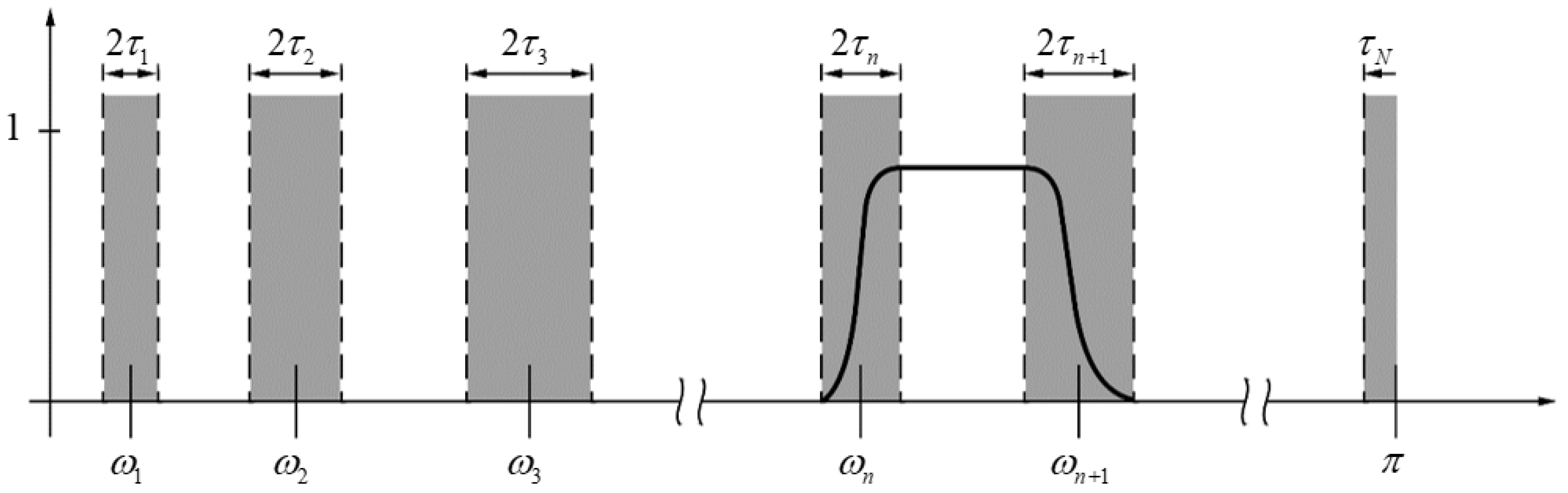
3.2. Spectrum Segmentation Based on Scale Space Method

After proposing the EWT, Gilles proposed a spectrum division method based on scale-space theory [22]. This method can quickly extract the mode of the median value of the spectrum and has the advantages of self-adaptability and no parameterization. In EWT, the boundary and number of band-pass filters greatly affect the results of signal decomposition and fault feature extraction.

Assuming that $\phi \left(x\right)$ is a function defined in the range of $\left[0,x_{\max }\right]$, the continuous scale-space representation $\psi \left(x,t\right)$ is determined by the convolution of the kernel function $\lambda \left(x;t\right)$ and $\phi \left(x\right)$:

$$\psi \left(x,t\right)=T_t\left[\phi \right]\left(x\right)=\lambda \left(x;t\right)\ast \phi (x)$$

(10)

where $\lambda \left(x;t\right)$ is the Gaussian kernel, given as, $\lambda \left(x;t\right)=\frac{1}{\sqrt{2\pi t}}{e}^{-x^2/(2t)}$, and t represents the scale parameter.

The scale-space representation of function $\phi \left(x\right)$, which can be understood as: $\psi \left(x,t\right)$, should be smoother when t increases, and all modes with characteristic lengths less than $\sqrt{t}$ will be eliminated. In practical applications, truncation is often used to obtain a filter, and the discrete scale space is expressed as follows:

$$\psi \left(m,t\right)={\displaystyle \sum _{n=-\mathrm{{\rm K}}}^{+\mathrm{{\rm K}}}\phi \left(m-n\right)\lambda \left(n;t\right)}$$

(11)

The discrete Gaussian kernel in Equation (11) is expressed as follows:

$$\lambda \left(n;t\right)=\frac{1}{\sqrt{2\pi t}}{e}^{-n^2/\left(2t\right)}$$

(12)

where $\mathsf{{\rm K}}$ is as large as possible so that the approximation error can be ignored. Usually $\mathsf{{\rm K}}=\alpha \sqrt{t}+1$($3\le \alpha \le 6$). When $\alpha =6$ the approximation error is less than 10⁻⁹.

In order to achieve discretization, the following discretization of scale parameters is also required:

$$\sqrt{t}=s\sqrt{t_0},s=1,\cdots ,S_{\max }$$

(13)

where $S_{\max }$ is an integer. Usually $\sqrt{t_0}=0.5$, and $S_{\max }=2x_{\max }$.

The size of the scale parameter t can change the spectrum division boundary. In other words, when the scale parameter t decreases, the more minimum points that are obtained, and the more spectral boundary points there are. When the scale parameter t increases, the spectral lines are smoother, fewer minimum points are obtained, and there are fewer spectral boundary points. Therefore, when the scale parameter is too small, for broadband signals such as a periodic transient impulse signal, the modulated frequency band disassembled easily, resulting in the destruction of the integrity of the periodic shock characteristics, which reduces the recognition accuracy of fault features. Because narrow-band filtering is more effective, the original scale parameter $\sqrt{t_0}=0.5$ is modified to $\sqrt{t_0}=2.0$.

In $\psi \left(m,t\right)$, the number of minimum points about the variable m is a decreasing function of the scale parameter t. If we suppose N0 is the initial number of minimum points, then each minimum point can generate a curve ${\mathsf{{\rm X}}}_i\left(i\in \left[1,N_0\right]\right)$ with length $L_i$.

The adaptive searching of Fourier spectrum segmentation points can be transformed into the searching of meaningful modes in the scale space. If the curve ${\mathsf{{\rm X}}}_i$ is long enough, that is, under a certain threshold T, when $L_i>T$ is satisfied, the minimum point corresponding to the curve ${\mathsf{{\rm X}}}_i$ is the boundary point of the modal in the scale space, which is precisely the Fourier spectrum segmentation boundary point. Then modes are quantified as determined by a threshold T so that the curve ${\mathsf{{\rm X}}}_i$ with a length greater than T is the boundary of spectrum segmentation, and meaningful modes are obtained. At present, there are five methods to determine automatically the threshold T: Mean, K-Means, Half-Normal, Otsu and Empirical-law. By analyzing and comparing the application effect of these five methods on the vibration signal of a bearing, this paper selects the Empirical-Law method to determine the threshold T.

3.3. Component Screening Based on KSES and CN

As the kurtosis index is more sensitive to single transient impact than to multiple periodic transient impact if the kurtosis index is adopted to judge the largest component of a periodic transient errors can easily occur. If the component of the fault impulse is reflected in the envelope spectrum, it will have obvious regularity, while the single impulse caused by a random fluctuation is irregular and unordered. Because of this property, the kurtosis index of the envelope spectrum (KES) approach is employed in component screening. However, because of noise, the envelope spectrum structure of the features of a fault can be submerged or contaminated with noise, so that its value is not different from that of other components, which is not conducive to screening. In this paper, we calculate the kurtosis index of the squared envelope spectrum (KSES) to highlight the fault characteristics and suppress other components. The squared envelope spectrum kurtosis can further highlight the difference between the periodic transient impact component and other components, which is easy to screen and has stronger robustness and adaptability.

In addition, the fault impulse is often modulated to more than one frequency band. There is a main resonance band and some number of sub-resonance bands, that is, there is a gap between the shock sequence and energy. As the correlation number (CN) can reflect the correlation and energy of each component and the original signal, we use the CN of each component and the corresponding original signal to screen components. The Pearson correlation coefficient is used here.

As mentioned in the previous section on EWT theory, each empirical mode component corresponds to a filter function. If the selected component is used directly, it may cause signal distortion. Therefore, this paper uses the inverse empirical wavelet transform (IEWT) to reconstruct the components to minimize signal distortion.

4. Algorithm Implementation Process

This paper proposes an algorithm based on sparse coding theory and AEWT to realize feature extraction and noise reduction of a bearing weak fault signal. The algorithm has the characteristics of self-adaptability, few unknown parameters, and high accuracy. Its implementation steps are shown in Figure 2.

(1)

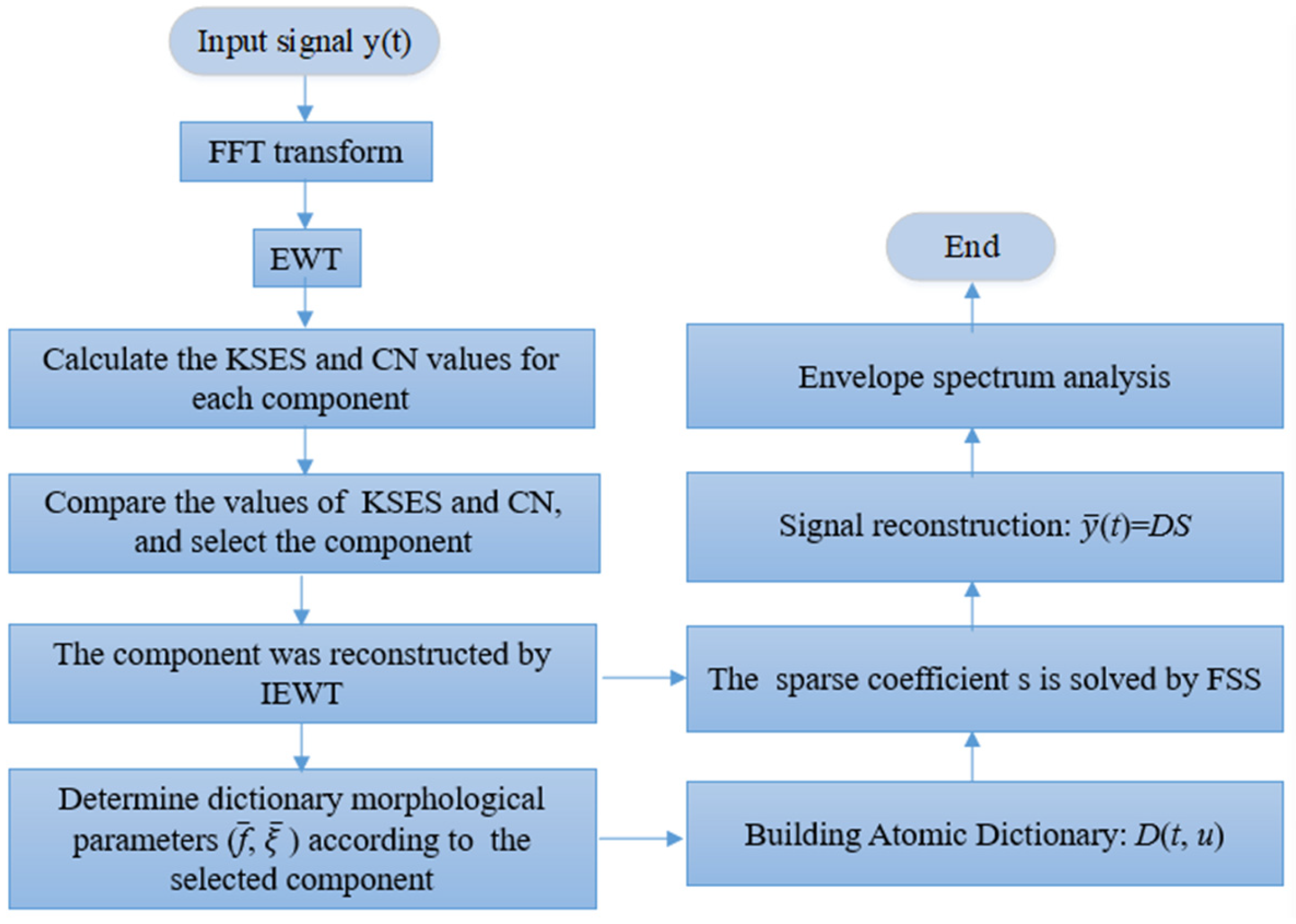
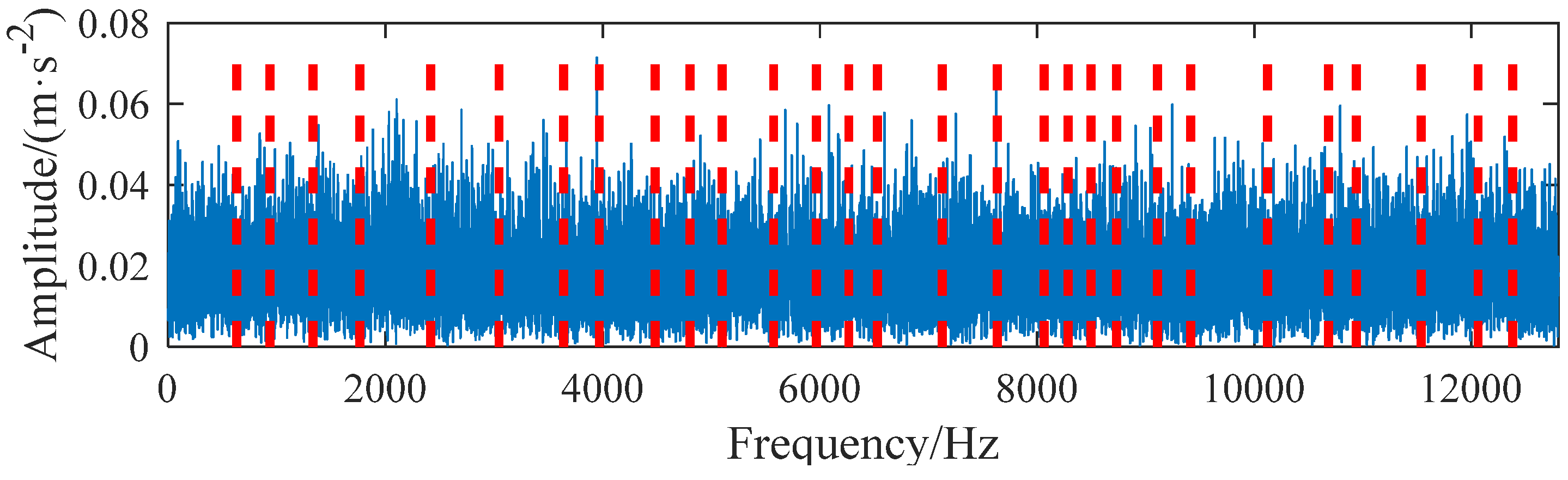
Firstly, the signal is transformed by FFT to obtain the Fourier spectrum. Then, the scale space method based on a rule of thumb is utilized to segment the spectrum adaptively, and the dividing points of each frequency band are obtained. Based on this, a wavelet filter bank is designed to decompose the signal and obtain component signals.

(2)

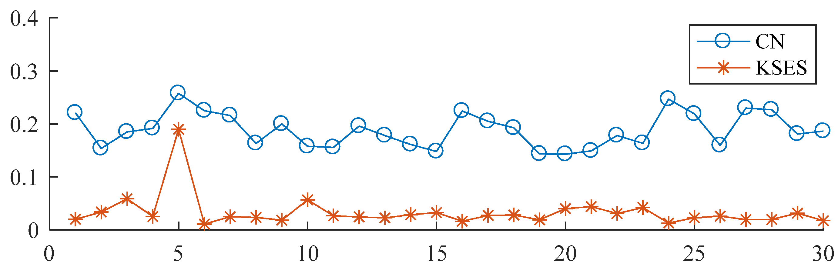
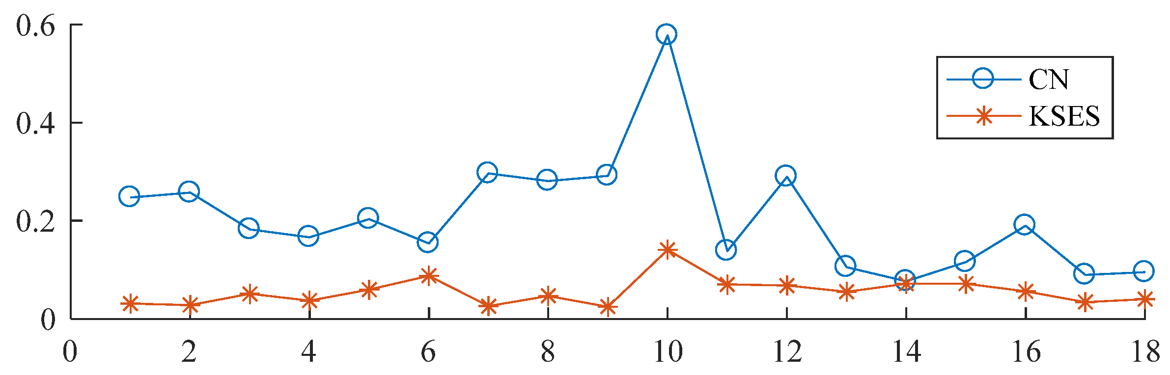
The KSES of each signal component and the cross-correlation coefficient with the original signal are calculated. The component with the highest KSES value and CN value is selected. According to the spectrum segmentation map, the resonance frequency band corresponding to the selected component is checked to see if it is segmented to determine whether it is necessary to merge the adjacent components. The selected components are inversely transformed by an empirical wavelet to obtain the signal $\overline{y}(t)$.

(3)

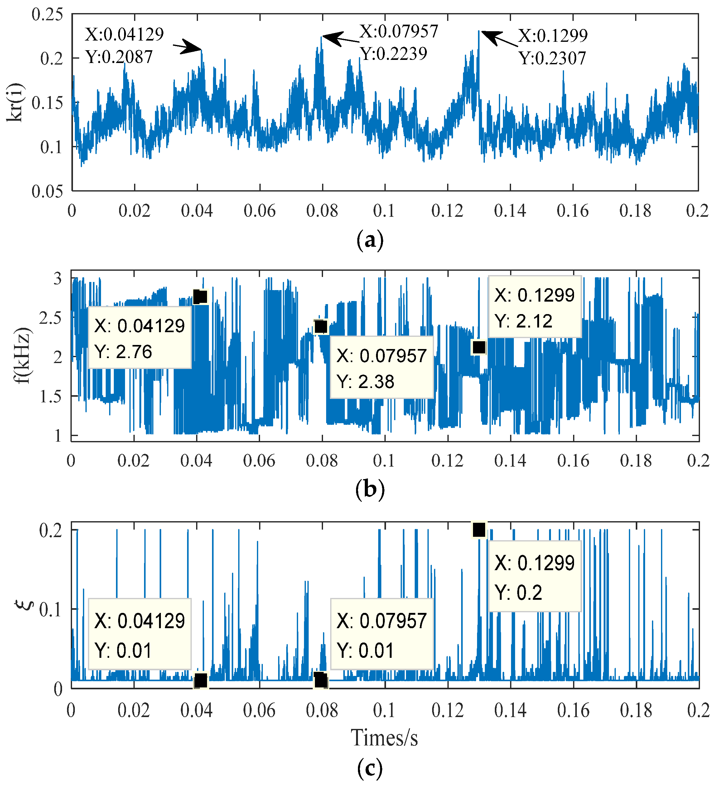
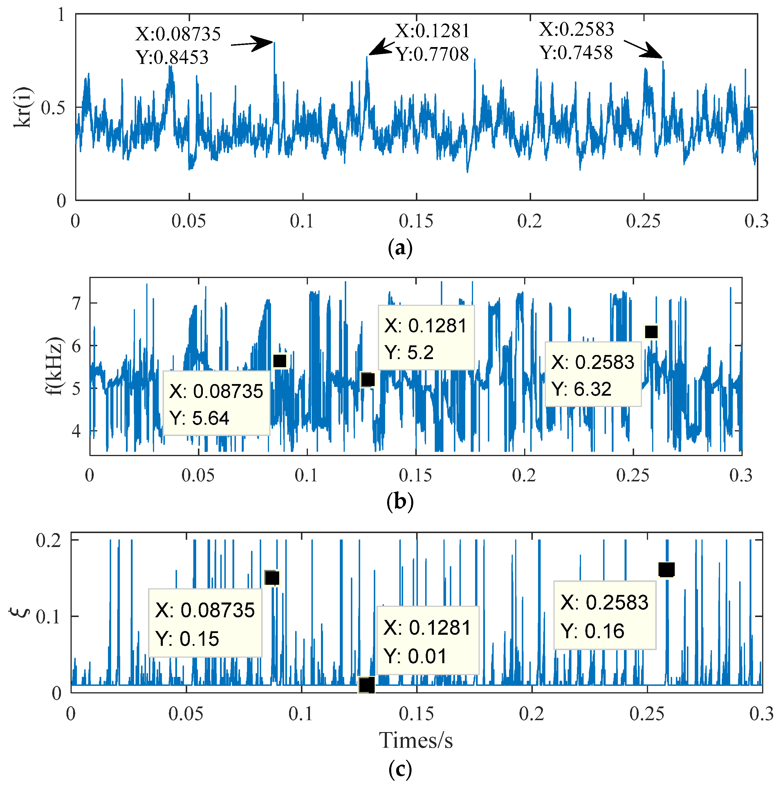
The peak frequency of the component frequency band is taken as the value of the resonance frequency parameter f of dictionary D. At the same time, the appropriate value in the range of damping ratio $\epsilon$ is selected, which needs to ensure that the basis function decays to zero over its own length.

(4)

According to the selected signal characteristic morphological parameters $\left(\overline{f},\overline{\epsilon }\right)$, it is brought into the basis function formula (4) and expanded according to the different time shift parameters u, and then the dictionary D is constructed. The value of u is $1/f_s$.

(5)

The signal $\overline{y}(t)$ and dictionary D are substituted into the FSS algorithm to calculate the sparse coefficient s. The sparse coefficient s and dictionary D are combined for sparse reconstruction to achieve signal reconstruction and noise reduction.

5. Simulation and Experimental Verification

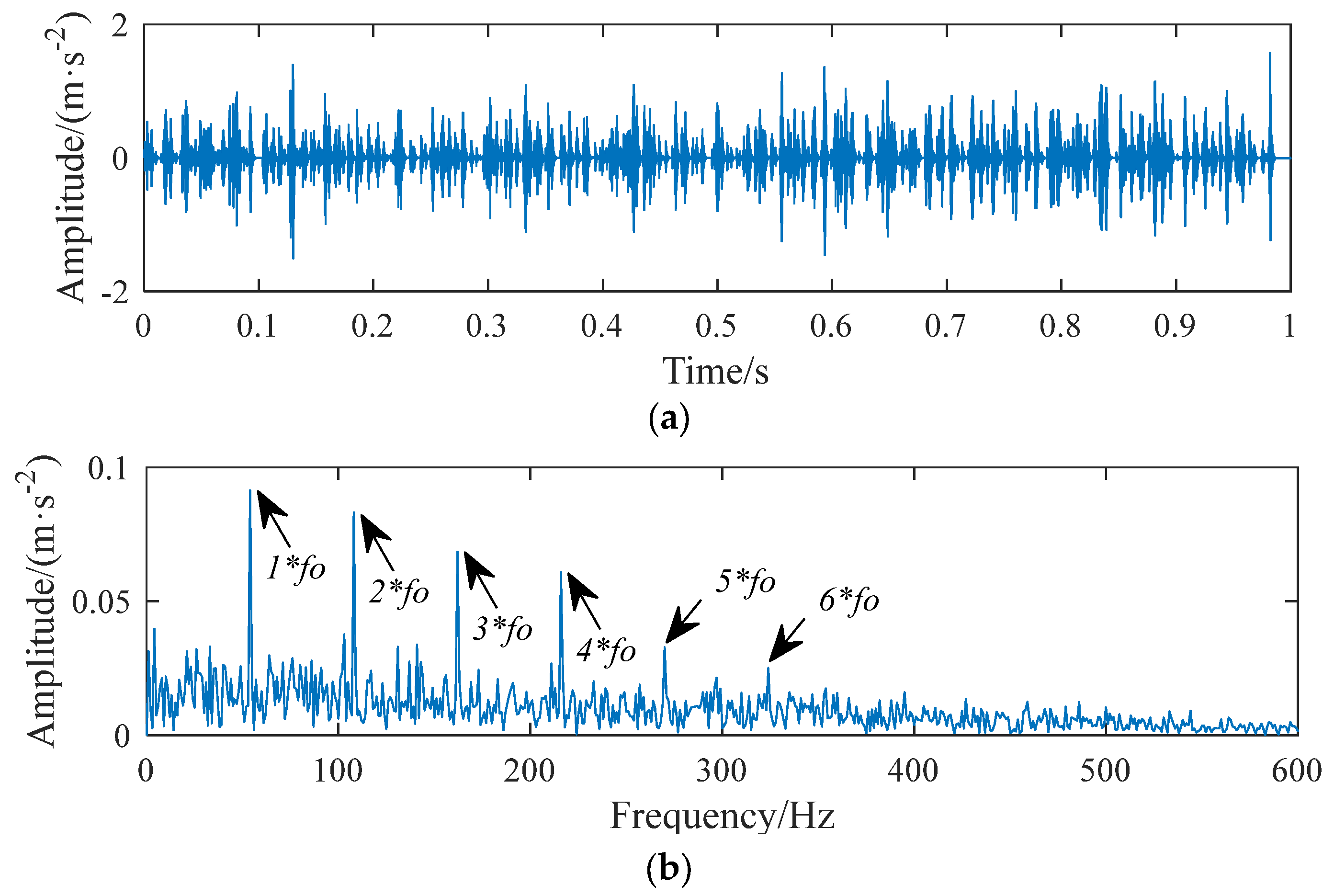
5.1. Simulation Verification

The simulation signal y (t) is constructed according to the characteristics of the internal ring of the rolling element and the outer ring of the rolling bearings when the peeling failure occurs. Its expression is [23,24]:

$$\mathrm{y}(t)={\displaystyle \sum _i^M{A}_{i}s(t-iT-{\tau }_i)}+n(t)$$

(14)

$$\left\{\begin{array}{c}{A}_i=A_0\cos (2\pi Qt+{\phi }_A)+{\mathrm{C}}_A\\ s\left(t\right)=e^{-Bt}\cos \left(2\pi ft+{\phi }_w\right)\end{array}\right.$$

(15)

where Ai is the modulation amplitude, whose period is 1/Q, Q is the rotation period (frequency fr = 1/Q), C_A is the amplitude random constant (C_A > A₀), $s(t)$ is the impact caused by pitting failure, T is the impact period, B is the attenuation coefficient, $f$ is the resonance frequency of the system, the random variable ${\tau }_i$ is the small sliding of the ith impact relative to the average period T, and n(t) represents the random noise.

The parameters of the outer ring fault simulation signal y_o(t) are set as: amplitude A_o = 2, sampling frequency f_s = 25,600 Hz, outer ring fault resonance frequency $f$ = 2000 Hz, attenuation coefficient 1000, fault characteristic frequency f_p = 54 Hz. The SNR of the added white Gaussian noise was −17 dB. The simulation fault signal with noise is shown in Figure 3.

The envelope spectrum of the simulated signal with noise is shown in Figure 4. The frequency component of the signal is very complex, and the fault characteristic frequency is submerged in the noise, making it difficult to distinguish. FFT is performed on the simulation signal to obtain the Fourier spectrum, and then EWT is performed based on the scale space method to obtain the spectrum segmentation, as shown in Figure 5. After decomposition, 30 empirical mode components are obtained in total, and their corresponding kurtosis values of the square envelope spectrum and cross-correlation coefficients with the original signal are calculated, respectively. Here, the KSES value is normalized for comparative analysis with the CN value, and the results are shown in Figure 6.

From the KSES and CN values, we can conclude that the fifth component is the one we need. From Figure 5 it can be seen that the frequency band of this component is positioned at 2000 Hz, which is consistent with the preset. At the same time, the frequency band of this component is not divided, and there is no need to merge other components.

To save calculation time and improve efficiency, the parameter range of correlation filtering is set here according to the decomposition result of EWT. The base atom also uses the Laplace wavelet, as does the subsequent verification. Its parameters are set as resonance frequency $F=\left\{1000:20:3000\right\}$, damping ratio $Z=\left\{0.01:0.005:0.2\right\}$, $T=\left\{0:1/f_s:0.2\right\}$, and support interval $w_s=470$. The result of the correlation filtering is shown in Figure 7. Looking at the correlation coefficient ${\kappa }_r$ between the simulated signal of the fault and the base atom, the higher peak point does not appear periodically, and it is not easy to judge whether it is the peak point corresponding to the fault shock signal. In this paper, the resonance frequency and damping ratio of three peak points with a higher ${\kappa }_r$ value are used to study this further. It can be seen that the resonance frequency f values of the three points are quite different, it is not easy to select the optimal value, and the optimal value deviates greatly from the set 2000 Hz. At the same time, the damping ratio tends to a lower value, which is inconsistent with the preset value. It shows that for a low signal-to-noise ratio signal, it cannot identify the correct damping ratio.

The waveform of the fifth component is shown in Figure 8. It can be seen that the SNR is still not high enough. The peak frequency of this component frequency band is 2104 Hz, which is taken as the value of f, the damping ratio $\psi =0.08$, the support interval $w_s=470$, and the time shift $\nu =1/f_s$.

The overcomplete dictionary D is constructed according to the determined parameters and is substituted into the FSS algorithm together with the fifth component signal to solve the sparse coefficient and reconstruct the signal. The SNR is greatly improved by observing the reconstructed waveform, as shown in Figure 9a. At the same time, from Figure 9b, the fault characteristic frequency and frequency doubling can be readily found. The fault characteristic frequency of 54 Hz obtained from the observation diagram is consistent with that of the fault characteristic frequency of 54 Hz set by simulation.

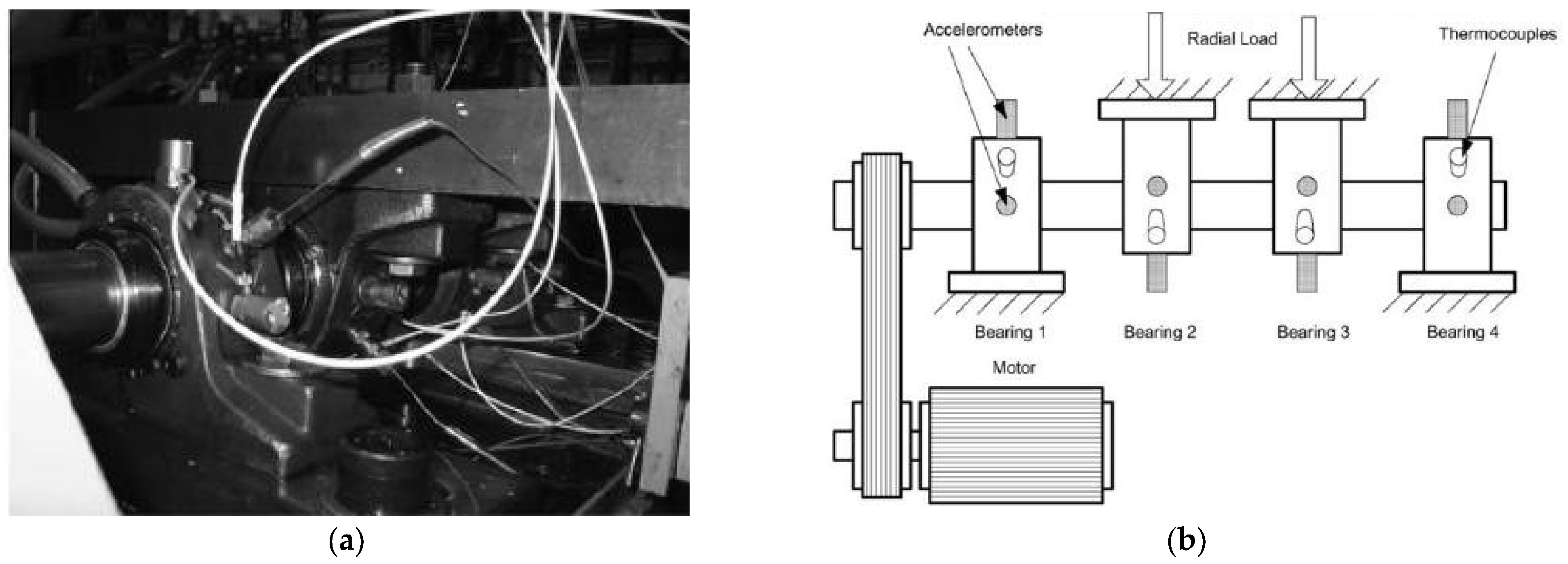
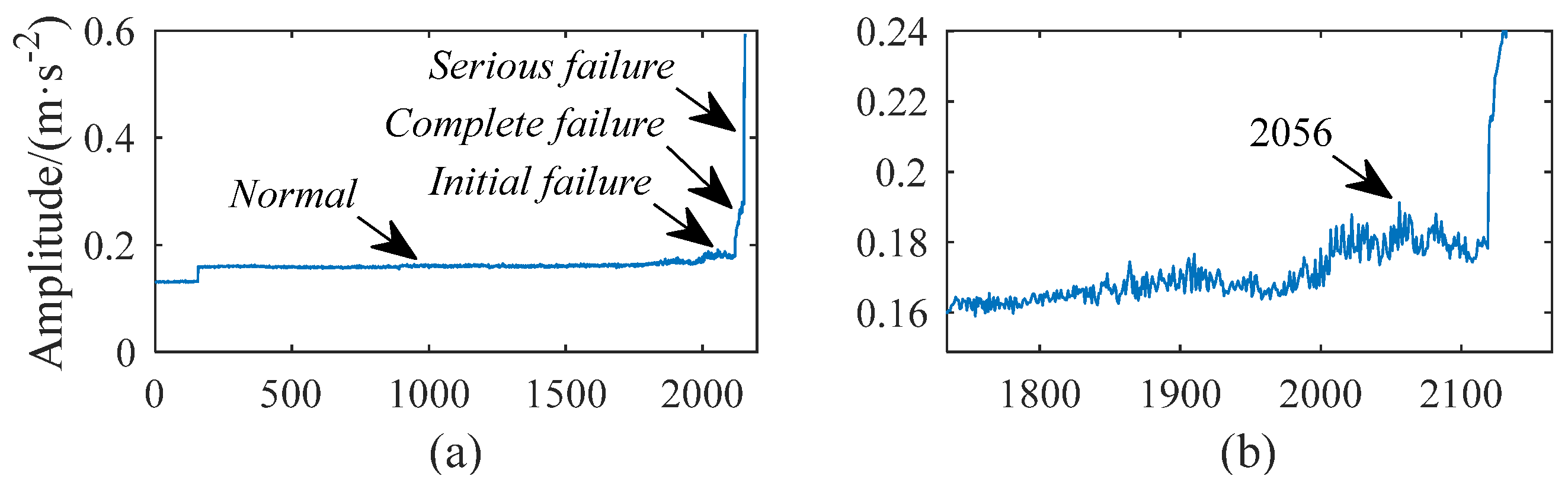
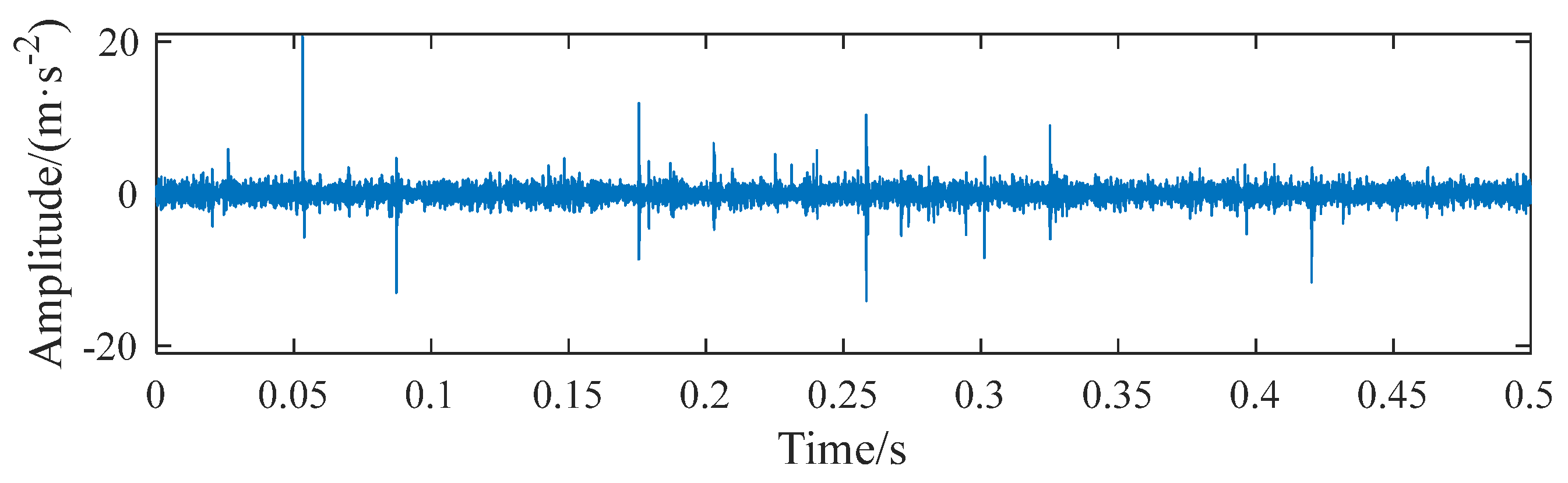
5.2. Experimental Verification

The experimental data are from the NASA diagnostic database and the rolling bearing life test data provided by the IMS center of the University of Cincinnati [25]. The test bench device is shown in Figure 10, and related parameters are shown in

Table 1. Relevant parameters of the test bearing.

Number of Rollers	Diameter of Roller	Pitch Diameter	Contact Angle	Sampling Frequency
16	8.407 mm	71.501 mm	15.17°	20 KZ

.

The sensor used in the test is a PCB353b33 piezoelectric acceleration sensor, and there are 20,480 data points in each run. Three groups of tests were carried out, and the whole life data of bearing three in data set 1 was selected as the experimental data. In the experiment, an inner ring-pitting fault occurred in the bearing. Similarly, the theoretical characteristic fault frequency f_i = 296.63 Hz is calculated according to relevant parameters.

The data collected in the horizontal direction of bearing 3, that is, the data collected in channel 5, were selected for analysis. There are 2156 groups of data, and the trend chart of root mean square (RMS) value in bearing 3 life cycle is drawn, as shown in Figure 11a. RMS is a common monitoring index in engineering and represents the energy of the vibration signal. By observing the change trend of the RMS value, it can be seen that the life cycle of the bearing inner ring consisted of four stages (trouble-free stage, initial failure stage, complete failure stage and catastrophic damage). When the bearing is in the initial fault stage, its amplitude does not change much; but over time, the vibration signal power spectrum will reflect a large increase in the amplitude of some frequency bands, which can be considered as the frequency band of the resonance frequency excited by the impact of the pitting fault. When the bearing is in the stage of complete failure, the impact may excite more high-frequency resonances unrelated to the impact until catastrophic bearing damage occurs. Therefore, for the whole life of bearing fault signals, we study the signal within the scope of the initial failure stage through KSES and CN to select the components, including periodic impact, then determine the value of the parameter f of the Laplace dictionary related to the resonance frequency generated by the shock. We then select the 2056th group of data belonging to the initial failure stage to verify the algorithm, as shown in Figure 11b.

The waveform of the 2056th set of data is shown in Figure 12, and the diagram of the corresponding envelope spectrum is shown in Figure 13. FFT is performed to obtain the spectrum, and then EWT is performed based on the scale space method to obtain the spectrum segmentation diagram, as shown in Figure 14. Eighteen components are obtained by EWT decomposition, whose KSES value and CN value are then calculated, as shown in Figure 15.

From the KSES and CN values, we can conclude that the 10th component is the one we need. Looking at the spectrum division (Figure 14), we can see that the component lies in the frequency band of about 5100 Hz. In addition, the resonant frequency band is not divided, so it is not necessary to combine the adjacent components. As can be seen from Figure 16, the kurtosis of the whole frequency band is the highest, and the best frequency band cannot be selected. The parameters of the correlation filtering method are resonance frequency $F=\left\{3500:20:7500\right\}$, damping ratio $Z=\left\{0.01:0.005:0.2\right\}$, $T=\left\{0:1/f_s:0.2\right\}$, and support interval $w_s=68$. The result is shown in Figure 17. Taking some peak points for analysis, it is similar to the simulated result before the application of the algorithm, and, thus, it is still not easy to get the correct values of the atomic morphological parameters.

The waveform of the 10th component is shown in Figure 18. It can be seen that the SNR is still not high enough. The peak frequency 5134 Hz of the component frequency band is taken as the value of parameter f, the damping ratio $\epsilon =0.07$, the support interval M = 68, and the time shift $\nu =1/f_s$. However, once the LWDFSS-AEWT algorithm is used to solve the coefficient and reconstruct the signal of the 10th component signal, as Figure 19a,b show, the noise is largely removed. The fault characteristic frequency extracted, 294 Hz, is close to the theoretical fault characteristic frequency of the inner ring, which is 296.63 Hz, so it can be judged that the bearing inner ring is faulty.

As a comparison, results obtained with this set of data using the SISC algorithm based on a learning dictionary, the BPDN algorithm based on the Symlet8 wavelet packet, and the WPT Kurtogram algorithm [26] are also presented, as shown in Figure 20, Figure 21 and Figure 22, respectively. Although the SISC algorithm based on a learning dictionary can get the base atom, the result is not ideal, as the matching degree between the base atom and the signal is not high. Although BPDN can extract the fault characteristic frequency and frequency doubling, the SNR is not high enough, and the reconstructed signal has poor results. The WPT Kurtogram can hardly distinguish the fault characteristic frequency. However, the LWDFSS-AEWT algorithm can obtain the ideal reconstructed signal and feature extraction results and is less affected by noise. Thus, the results show the advantages of frequency band division and the accuracy of frequency band selection by the AEWT method.

6. Conclusions

This paper proposes a fault detection method for rolling bearing weak faults based on an optimized LWD and the FSS algorithm. This method uses the Laplace wavelet to construct a sparse dictionary, and obtains the resonance frequency from the signal by AEWT based on the scale space method and combined component screening, then determines the morphological parameters of the Laplace wavelet. The signal-to-noise ratio is then improved, and the sparse signal is reconstructed. Simulation and experiment show that the envelope analysis of the reconstructed sparse signals obtained by this method can successfully extract and highlight the weak fault characteristic frequencies of bearings under strong background noise interference to allow the diagnosis of rolling bearing faults. At the same time, the proposed LWDFSS-AEWT algorithm is compared with the SISC algorithm based on a learning dictionary, the BPDN algorithm based on the Symlet8 wavelet packet and the WPT Kurtogram algorithm. The results of the comparison show the superiority of the LWDFSS-AEWT algorithm. As the algorithm utilizes the characteristics of the signal for feature extraction, it can be predicted that the method can be extended to the fault diagnosis of other rotating machinery, such as gears.

References

1. Chen, J.; Pan, J.; Li, Z.; Zi, Y.; Chen, X. Generator bearing fault diagnosis for wind turbine via empirical wavelet transform using measured vibration signals. Renew. Energy 2016, 89, 80–92. [Google Scholar] [CrossRef]
2. Olshausen, B.A.; Field, D.J. Emergence of simple-cell receptive field properties by learning a sparse code for natural images. Nature 1996, 381, 607–609. [Google Scholar] [CrossRef] [PubMed]
3. Abrol, V.; Sharma, P.; Sao, A.K. Greedy double sparse dictionary learning for sparse representation of speech signals. Speech Commun. 2016, 85, 71–82. [Google Scholar] [CrossRef]
4. Lin, N.; Sun, H.; Zhang, X.P. Overlapping Animal Sound Classification Using Sparse Representation. In Proceedings of the ICASSP 2018—2018 IEEE International Conference on Acoustics, Speech and Signal Processing (ICASSP), Calgary, AB, Canada, 15–20 April 2018. [Google Scholar]
5. Mairal, J.; Elad, M.; Sapiro, G. Sparse Representation for Color Image Restoration. IEEE Trans. Image Process. 2007, 17, 53–69. [Google Scholar] [CrossRef] [PubMed] [Green Version]
6. Zhu, Z.; Yin, H.; Chai, Y.; Li, Y.; Qi, G. A novel multi-modality image fusion method based on image decomposition and sparse representation. Inf. Sci. 2018, 432, 516–529. [Google Scholar] [CrossRef]
7. Feng, Z.; Zhou, Y.; Zuo, M.J.; Chu, F.; Chen, X. Atomic decomposition and sparse representation for complex signal analysis in machinery fault diagnosis: A review with examples. Measurement 2017, 103, 106–132. [Google Scholar] [CrossRef]
8. Zhang, Y.; Xu, B.; Zhou, N. A novel image compression–encryption hybrid algorithm based on the analysis sparse representation. Optics Commun. 2017, 392, 223–233. [Google Scholar] [CrossRef]
9. Du, Z.; Chen, X.; Zhang, H.; Yan, R. Sparse Feature Identification Based on Union of Redundant Dictionary for Wind Turbine Gearbox Fault Diagnosis. IEEE Trans. Ind. Electron. 2015, 62, 6594–6605. [Google Scholar] [CrossRef]
10. Wang, H.; Du, W. Fast Spectral Correlation Based on Sparse Representation Self-Learning Dictionary and Its Application in Fault Diagnosis of Rotating Machinery. Complexity 2020, 2020, 9857839. [Google Scholar] [CrossRef]
11. Kong, Y.; Wang, T.Y.; Feng, Z.P.; Chu, F.L. Discriminative dictionary learning based sparse representation classification for intelligent fault identification of planet bearings in wind turbine. Renew. Energy 2020, 152, 754–769. [Google Scholar] [CrossRef]
12. Li, J.M.; Wang, H.; Wang, X.D.; Zhang, Y.G. Rolling bearing fault diagnosis based on improved adaptive parameterless empirical wavelet transform and sparse denoising. Measurement 2020, 152, 14. [Google Scholar] [CrossRef]
13. He, G.; Ding, K.; Lin, H. Fault feature extraction of rolling element bearings using sparse representation. J. Sound Vib. 2016, 366, 514–527. [Google Scholar] [CrossRef]
14. Tang, H.; Chen, J.; Dong, G. Sparse representation based latent components analysis for machinery weak fault detection. Mech. Syst. Signal Process. 2014, 46, 373–388. [Google Scholar] [CrossRef]
15. Zhou, H.X.; Li, H.; Liu, T.; Chen, Q. A weak fault feature extraction of rolling element bearing based on attenuated cosine dictionaries and sparse feature sign search. ISA Trans. 2020, 97, 143–154. [Google Scholar] [CrossRef]
16. Gilles, J. Empirical Wavelet Transform. Signal Process. IEEE Trans. 2013, 61, 3999–4010. [Google Scholar] [CrossRef]
17. Chegini, S.N.; Bagheri, A.; Najafi, F. Application of a new EWT-based denoising technique in bearing fault diagnosis. Measurement 2019, 144, 275–297. [Google Scholar] [CrossRef]
18. Song, Y.; Zeng, S.; Ma, J.; Guo, J. A Fault Diagnosis Method for Roller Bearing Based on Empirical Wavelet Transform Decomposition with Adaptive Empirical Mode Segmentation. Measurement 2017, 117, 266–276. [Google Scholar] [CrossRef]
19. Cao, H.; Fan, F.; Zhou, K.; He, Z. Wheel-bearing fault diagnosis of trains using empirical wavelet transform. Measurement 2016, 82, 439–449. [Google Scholar] [CrossRef]
20. Jiang, Y.; Zhu, H.; Li, Z. A new compound faults detection method for rolling bearings based on empirical wavelet transform and chaotic oscillator. Chaos Solitons Fractals 2016, 89, 8–19. [Google Scholar] [CrossRef]
21. Wang, S.; Huang, W.; Zhu, Z.K. Transient modeling and parameter identification based on wavelet and correlation filtering for rotating machine fault diagnosis. Mech. Syst. Signal Process. 2011, 25, 1299–1320. [Google Scholar] [CrossRef]
22. Gilles, J.M.; Heal, K. A parameterless scale-space approach to find meaningful modes in histograms—Application to image and spectrum segmentation. Int. J. Wavelets Multiresolut. Inf. Process. 2014, 12, 1450044. [Google Scholar] [CrossRef]
23. Mcfadden, P.D.; Smith, J.D. Model for the vibration produced by a single point defect in a rolling element bearing. J. Sound Vib. 1984, 96, 69–82. [Google Scholar] [CrossRef]
24. Mcfadden, P.D.; Smith, J.D. The vibration produced by multiple point defects in a rolling element bearing. J. Sound Vib. 1985, 98, 263–273. [Google Scholar] [CrossRef]
25. Qiu, H.; Lee, J.; Lin, J.; Yu, G. Robust performance degradation assessment methods for enhanced rolling element bearing prognostics. Adv. Eng. Inform. 2003, 17, 127–140. [Google Scholar] [CrossRef]
26. Lei, Y.; Jing, L.; He, Z.; Zi, Y. Application of an improved kurtogram method for fault diagnosis of rolling element bearings. Mech. Syst. Signal Process. 2011, 25, 1738–1749. [Google Scholar] [CrossRef]
Figure 1. Fourier spectrum segmentation.
Applsci 12 10807 g001
Figure 2. Flowchart of Algorithm for Feature Extraction of Weak Faults of Rolling Bearings.
Applsci 12 10807 g002
Figure 3. Simulated fault signal with noise.
Applsci 12 10807 g003
Figure 4. Envelope spectrum of the simulated outer ring fault signal with SNR = −17 dB.
Applsci 12 10807 g004
Figure 5. Adaptive spectrum segmentation.
Applsci 12 10807 g005
Figure 6. CN and KSES values of each component.
Applsci 12 10807 g006
Figure 7. Correlation filtering result of original signal: (a) The correlation coefficient κ r between the base atom and the original signal; (b) Resonance frequency of each point in κ r ; and (c) Damping ratio of each point in κ r .
Applsci 12 10807 g007
Figure 8. Time domain waveform of the fifth component.
Applsci 12 10807 g008
Figure 9. The result of SNR = −17 dB simulation signal processing based on the LWFSS-AEWT algorithm: (a) Time domain waveform of reconstructed signal; and (b) Envelope spectrum of the reconstructed signal.
Applsci 12 10807 g009
Figure 10. Illustration of the test device: (a) Testbed of rolling element bearings; and (b) Schematic diagram of the bearing test bench.
Applsci 12 10807 g010
Figure 11. RMS value trend graph and partially enlarged graph of bearing 3 full life data: (a) RMS value trend graph; and (b) Partially enlarged graph.
Applsci 12 10807 g011
Figure 12. The waveform of the 2056th set of data.
Applsci 12 10807 g012
Figure 13. Envelope spectrum of the 2056th set of data.
Applsci 12 10807 g013
Figure 14. Schematic diagram of spectrum division of the envelope spectrum of the 2056th set of data.
Applsci 12 10807 g014
Figure 15. CN and KSES values of each component of the envelope spectrum of the 2056th set of data.
Applsci 12 10807 g015
Figure 16. Fast spectral kurtosis figure of the 2056th set of data.
Applsci 12 10807 g016
Figure 17. Correlation filtering result of the 2056th set of data: (a) The correlation coefficient κ r between the base atom and the original signal; (b) Resonance frequency of each point in κ r ; and (c) Damping ratio of each point in κ r .
Applsci 12 10807 g017
Figure 18. The waveform of the 10th component.
Applsci 12 10807 g018
Figure 19. The result of the 2056th set of data processing based on LWDFSS-AEWT algorithm: (a) Waveform of reconstructed signal; (b) Envelope spectrum of the reconstructed signal.
Applsci 12 10807 g019
Figure 20. Results obtained with SISC based on a learning dictionary: (a) is the base atom obtained by learning; and (b) is the envelope spectrum of the reconstructed signal corresponding to the atom.
Applsci 12 10807 g020
Figure 21. Reconstructed signal and its envelope spectrum obtained by BPDN algorithm based on the Symlet8 wavelet packet.
Applsci 12 10807 g021
Figure 22. The reconstructed signal and its envelope spectrum obtained based on the WPT Kurtogram algorithm.
Applsci 12 10807 g022