1. Introduction
Machine condition monitoring currently arouses great interest among researchers and a widely defined industry. In modern industrial applications, the aim is to ensure the highest possible level of safety. Control structures are equipped with automatic diagnostics systems. The elements whose failure can lead to a catastrophe include electric motors. Currently, the most popular in this group are permanent magnet synchronous motors (PMSM). The control system, in the case of PMSM, requires stator currents and rotor speed sensors. Those sensors allow for the stable operation of the drive system in a wide range of speed changes. Particularly important is the position/speed sensor. Determining the position of the shaft is necessary to control the PMSM. For this reason, the diagnostics of measuring sensors are as important as the diagnostics of other motor components [
1]. In the PMSM drive system for speed measurement resolvers, encoders and tachometric sensors are mostly used. Damage to these types of elements may be divided into four main categories [
2]:
Intermittent or total loss of signal;
Constant fault, where the measured signal takes a constant value, despite the motor rotation (the error may result from malfunctioning electronics or data acquisition system);
Gain fault, where the measured signal is reduced or amplified in relation to the real value (error due to inappropriate scaling);
Signal interference (in the case of the resolver and tachometer sensor, these are measurement noises appearing in analog signals, while in the encoder, such disturbances may arise during the cyclic loss of pulses).
In the subject of damage to the speed sensor in the drive system with an electric motor, mainly one approach is described. State variable observers and comparative diagnostics are used. The estimated signal is compared with the measured value. When the difference between the estimated and measured value exceeds a certain constant, the detector indicates a failure, and the system is switched to a sensorless operation based on the estimated value [
3,
4,
5,
6,
7,
8,
9,
10,
11,
12].
Most of the works describe only simulation results. This is due to the fact that even a short loss of the correct measurement of the shaft position can lead the system out of stability. An example of such work is [
2]. The authors proposed the detection of speed sensor damage using the high-order sliding mode observer. Simulation results are shown for several speed values, with the system under load, for two types of failures—constant fault and measurement noise. In the case of constant fault, detection with a significant increase in speed is shown; the reaction of the detection system to small changes in speed is unknown. During measurement noise, the detector pulses, which can be difficult to interpret in a practical application. Paper [
3] also presents the simulation results for a detection mechanism of the same type, but only the constant fault failure was considered, and the Unknown input observer was used to estimate the speed. A slight modification of this approach is presented in [
4]. Comparing the measured and estimated values was also applied for damage detection. In this case, the extended Kalman filter (KF) was used. The modification is switching the controller after a failure occurrence to a fuzzy logic controller. The simulation results show that during a small discrepancy between the measured and estimated speeds caused by a failure, the system can operate with a robust controller and does not require switching to sensorless mode. In the literature, it is also possible to find works using other types of estimators, such as model reference adaptive system (MRAS) [
12] and the Luenberger observer (LO) [
9]. The main disadvantage of the described solutions is the lack of experimental research.
The use of other types of methods is shown in single articles. In [
13], detection is based on the park current vector (PCV). This solution allows to detect the loss of the measurement signal. This is one of the few papers where both simulation and experimental results are included. The concept of a neural detector is shown in [
14]. The detection is based on measured and estimated signals. However, this solution is presented for an induction motor, with only simulation results. The obtained results show that the detection of damage to the speed sensor using a neural network allows for high efficiency.
In the literature, many examples where neural detectors are used in drive systems for faults of elements other than the speed sensor can be found. These works show mainly applications for detecting electrical [
15,
16] and mechanical [
17,
18] damage to the motor itself. In the case of sensors, several works describe the detection of damage to current sensors using neural networks [
19,
20,
21]. These works confirm the effectiveness of such solutions, which is why it is the next step to use neural detection to damage the speed sensor.
The paper presents a proposal to extend diagnostic systems based on estimators of state variables with damage classification of any speed sensor type. For this purpose, a shallow neural network was used. Such an approach has not been previously described in the literature. The work is focused on the possibilities of using neural networks in the classification of faults of current sensors. The speed estimators used in the work are described as indirect tools. The influence of estimator parameters on estimation accuracy has already been discussed many times in the literature [
22,
23,
24].
The use of NN not only allows for classifying the type of damage but also increases the effectiveness of the 0–1 fault detection. Additional diagnostic functionality allows for obtaining additional information about the failure. Which in practice means a faster repair of the damaged element. Three types of failures are considered in the system, which can most often occur in the speed sensor—loss of signal, scaling error, and signal interference. These failures usually have repeatable causes. Such initial diagnostics can significantly speed up the repair process of an element or determine whether it needs to be replaced. The paper shows experimental results that distinguish the proposed work from other works describing the detection of speed sensor faults. The results are presented for different speed and load values. In addition, the article presents an analysis of the damage classifier based on the SMO and MRAS estimators to compare both systems. For both systems, the MLP was used for damage classification.
The article is organized as follows. The first part presents the importance of the research problem and describes it against the background of works available in the literature. The next part describes the theoretical background of state variable observers used for fault detection. The third chapter presents the process of designing a neural speed sensor fault classifier using state variable observers described in chapter two. The following parts present the results obtained from experimental tests. Finally, the last chapter contains a brief summary of the obtained results.
2. Control Structure and State Variable Observers Used in the Research
In this work, two types of speed estimators were used to conduct a comparative analysis. The control system is equipped with a simple fault detector that compares the measured and estimated speed values. The detection is also based on comparing the measured and estimated values of the current in the q axis in the rotor frame. The use of observers allows for sensorless operation after a failure and fast fault detection.
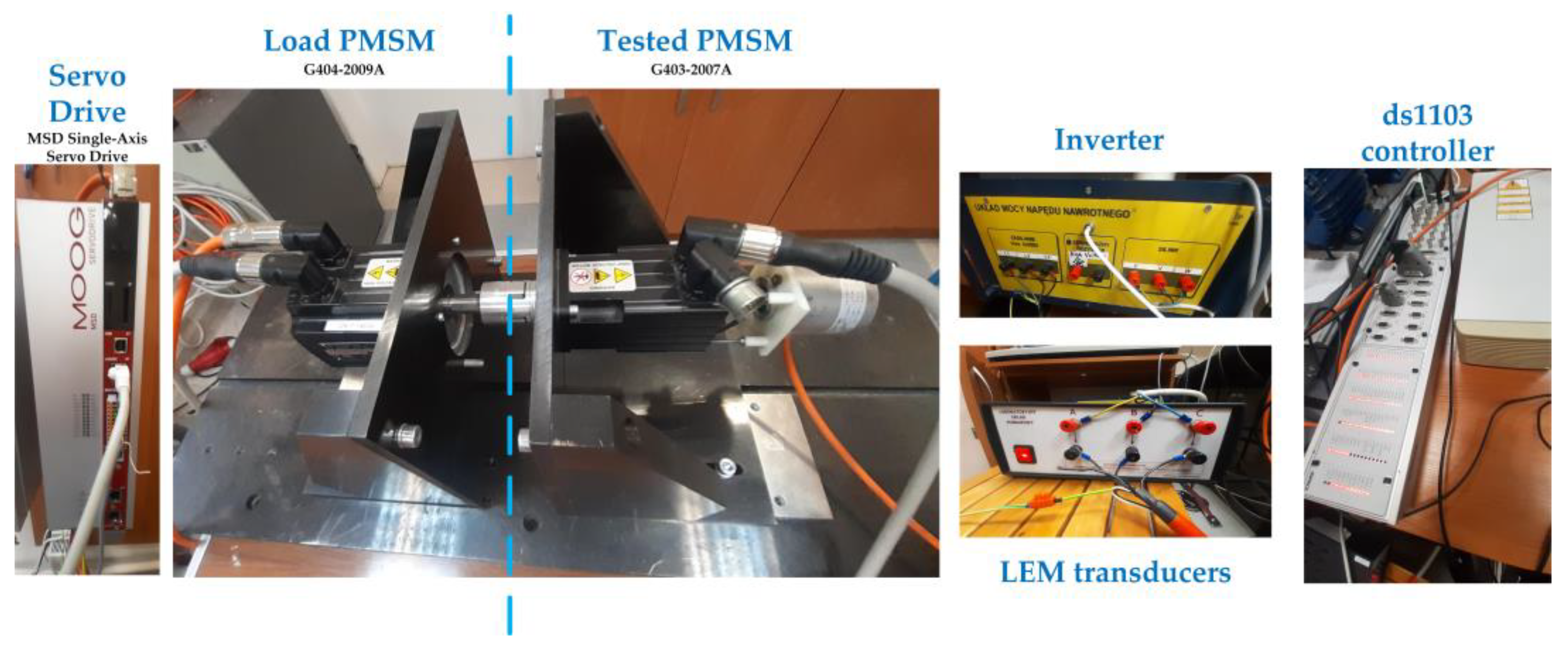
Experimental tests were carried out on a 0.894 kW PMSM motor from Moog (G403-2007A). The dSpace DS1103 rapid prototyping system with Control Desk and Matlab/Simulink software was used in the tests, the position of the shaft was measured with an incremental encoder (36,000 imp./rev), and the current measurement was carried out using LEM-type current transducers. Another Moog PMSM motor (G404-2009A—0.89 kW) controlled by a Moog servo drive was used as the load. The parameters of the motor are presented in
Table 1.
Photos of the essential elements of the laboratory set-up are shown in
Figure 1.
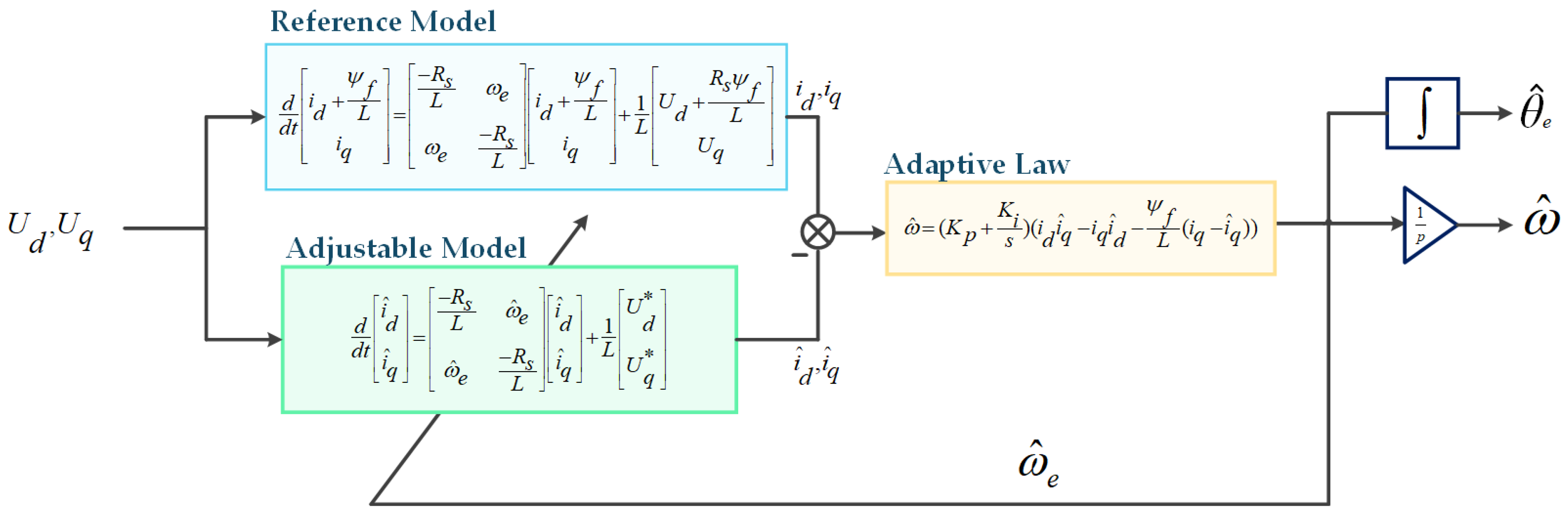
2.1. Model Reference Adaptive System
The first system used for speed estimation is the model reference adaptive system (MRAS). This type of estimator consists of three basic elements: reference model, adjustable model, and adaptive law. The difference between the value obtained from the reference model and the adjustable model is processed by the adaption law. Subsequently obtained signal can adjust the adjustable model parameters and strive to obtain the same value as the value from the reference model. MRAS used in the article is based on the PMSM model in the
d-q coordinate system, assuming that the motor is equipped in surface mounted magnets and inductances
[
22]:
where
, —currents in d-q coordinate;
—magnetic flux;
—stator inductance;
—stator resistance;
, —voltages in d-q coordinate;
—electrical speed.
In the following, for the sake of simplifying the notation, the following relationship was assumed:
The adjustable model is based on Equations (1) and (2), where the adaptive parameter is electrical speed
. The actual measurement of the
,
currents is selected as the reference model. The excitatory signals for both models are the
,
voltages. The final equation is presented below as follows:
where
, —estimated currents in d-q coordinate;
—estimated electrical speed.
The last element of the MRAS is adaptive law. In the study, adaptive law based on the following equation was used:
In the research, adaptive law parameters
= 0.6 and
= 200 were adopted.
Figure 2 shows the complete estimation scheme based on MRAS.
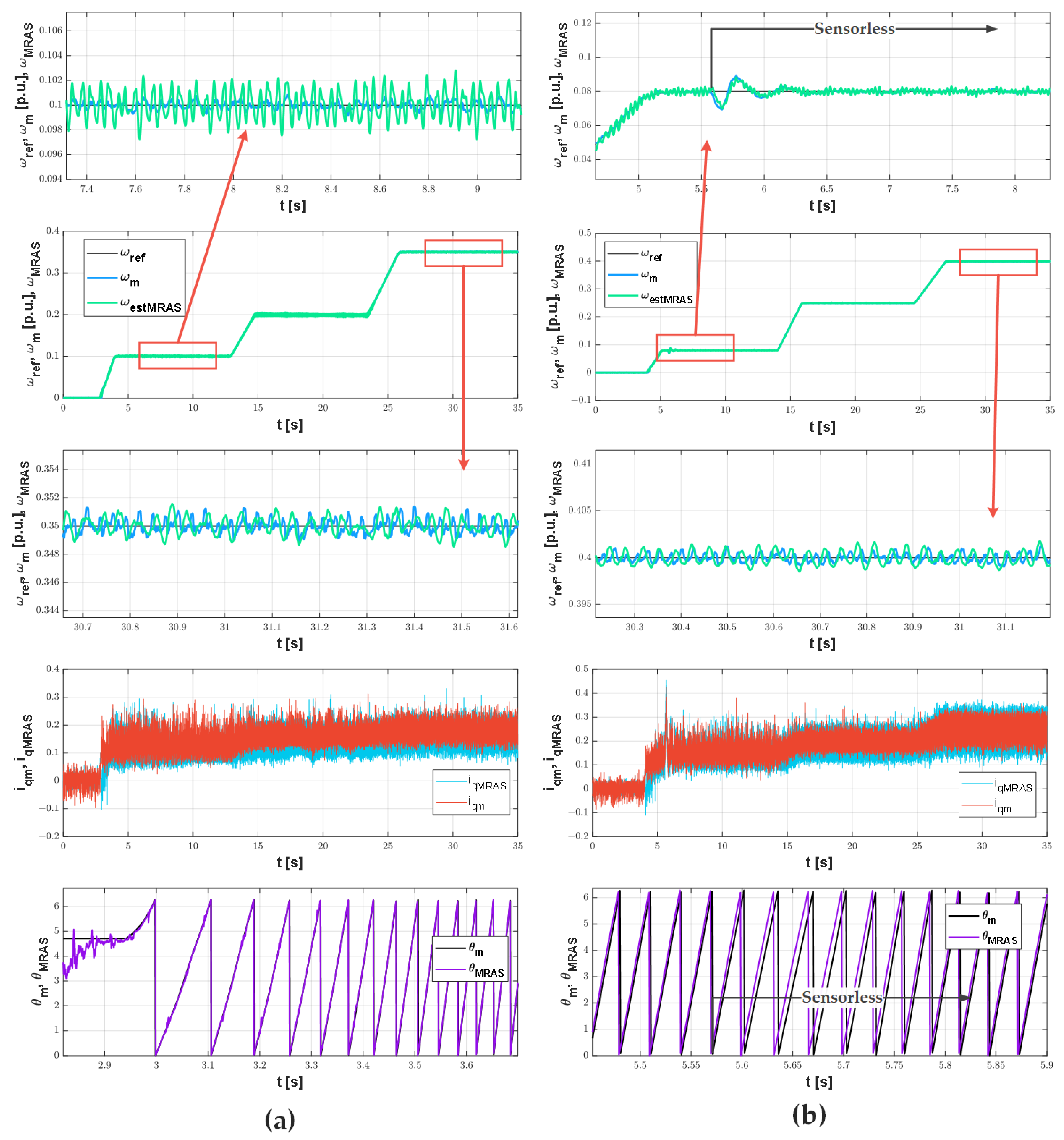
Example transients obtained from the experimental set-up of the estimated and measured speed in the sensor and sensorless mode operation are shown in
Figure 3. Speed is estimated with high accuracy. The system works stably in sensorless mode.
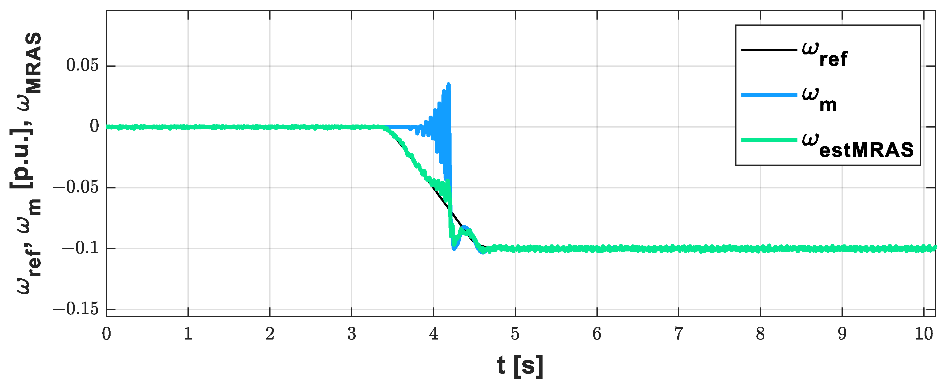
The MRAS system also enables sensorless startup. The course of such a start is shown in
Figure 4.
2.2. Sliding Mode Observer
Sliding mode observer (SMO)used in article is based on PMSM model in
α-β coordinate system, defined below:
where
, —currents in α-β coordinate;
,—voltages in d-q coordinate.
In the case of SMO, the basis for the speed estimation is the estimation of the back-EMF expressed as follows:
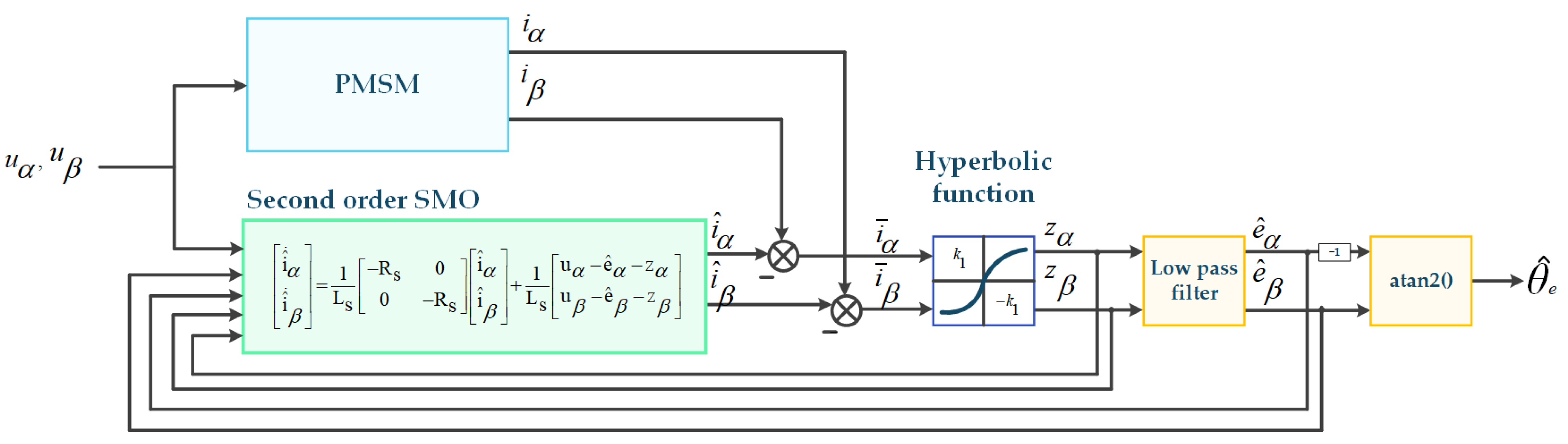
From these equations, it can be concluded that the electrical speed value can be determined if the values of the back-EMF voltage are available. Since these components cannot be directly measured during motor control, an observer is required. For this purpose, the reduced order back-EMF SMO will be used, which is defined as follows:
where superscript (ˆ) indicates that the value is observed, and
zα and
zβ are the SMO feedback signals. In the case of this observer, it also attempted to equalize the estimated and measured currents:
and
. The observation errors are defined as follows:
where
are the errors between the measured and the observed stator currents.
The sliding surface defined for the SMO is given by (10). It means that the phase plane is divided into two sections in which the observation errors defined in (9) have different signs. The switching action occurs as follows:
The current observation errors are used as the input for the switching function. In the early stages of the SMO, the discontinuous sign function was commonly used [
25]. However, the sign function introduces a lot of noise and chattering. Modern solutions use continuous functions as the limit, sigmoid or hyperbolic functions [
26]. In this article, a hyperbolic function will be used, and it is defined as follows:
where
—the feedback gain;
is—the shaping parameter.
The short time interval average values of the feedback signal components in (11) represent the back-EMF components. To obtain these values, a low-pass filter (LPF) can be used, which is defined as follows [
26]:
where
is the cutoff frequency of the LPF. Rearranging Equation (8), the estimated electrical rotor position can be calculated as follows:
The estimated mechanical speed can be calculated by deriving the observed rotor position:
The block diagram of the reduced-order SMO is presented in
Figure 5.
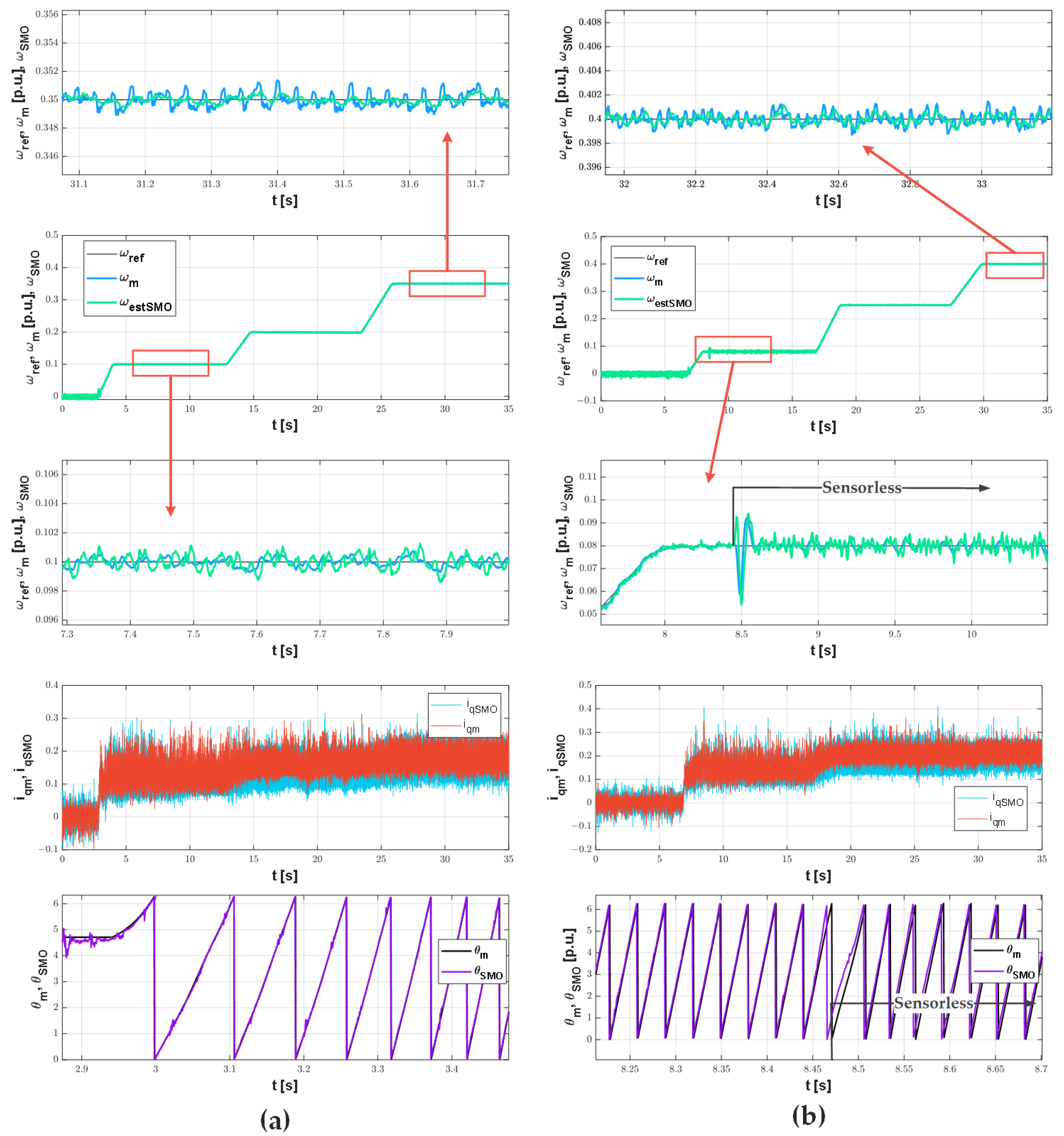
Example transients of estimated and measured speed in sensor and sensorless mode are presented in
Figure 6. The results confirm stable operations in a sensorless system.
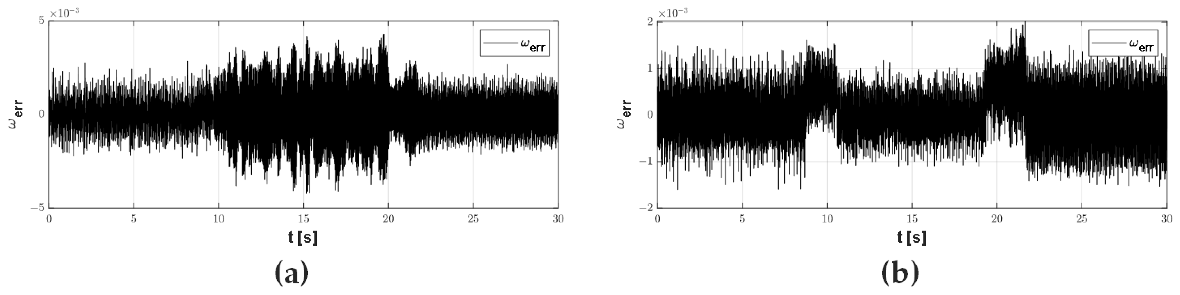
In order to compare the estimation accuracy of both systems,
Figure 7 shows the estimation error transients (difference between measured and estimated speed) for both systems under the same operating conditions. Based on the presented results, it can be concluded that the SMO system achieves greater accuracy.
3. Speed Sensor Faults Classifier Based on Neural Networks
The damage classification mechanism is based on the classic multilayer perceptron. The perceptron is a feedforward neural network consisting of an input layer, n- hidden layers, and an output layer. Each neuron in each layer is connected to a neuron in the next layer; there are no connections between the neurons of the same layer. The operation of such a neural network can be written in a simple way by the equation [
17]:
where
yk—k-th output of the network;
xj—j-th input of the network;
—weights of the first and second hidden layers, respectively;
—biases in the first and second hidden layers, and output layer, respectively;
—activation functions of first hidden layer, second hidden layer, and output layer, respectively.
The paper presents two types of speed sensor fault neural classifiers based on two different speed observers. Classifiers are presented as two separate neural structures. Apart from the use of two different types of observers, the classification schemes are the same. In both cases, the Levenberg–Marquardt method was used to train the network.
Moreover, 23-15-1 was chosen as the network structure according to the theory with the highest efficiency with the number of neurons in the first hidden layer 2N + 1.
The basic element while designing this type of damage classifier is the selection of appropriate diagnostic signals. The input vector of the neural network is based on the measured and estimated speed value, as well as the measured and estimated q-axis current value.
The difference between the current and previous samples is given to the input of the neural network. A simple comparative detector is primarily responsible for damage detection. The value of the measured and estimated speed and the value of the current in the
q axis are compared. The output value of this detector activates the sensorless mode. This signal is also fed to the input of the neural network. The full input vector is presented below:
The description of individual input signals is presented in
Table 2.
The classifier consists of one output, which indicates faults and is defined as follows:
0—no fault;
1—signal interference;
2—scaling error;
3—signal loss.
In addition to the listed failures, the system can also detect the disappearance of individual pulses of the detector. Training the network for a signal loss is sufficient for the detector to consider this type of failure as well.
4. Experimental Results
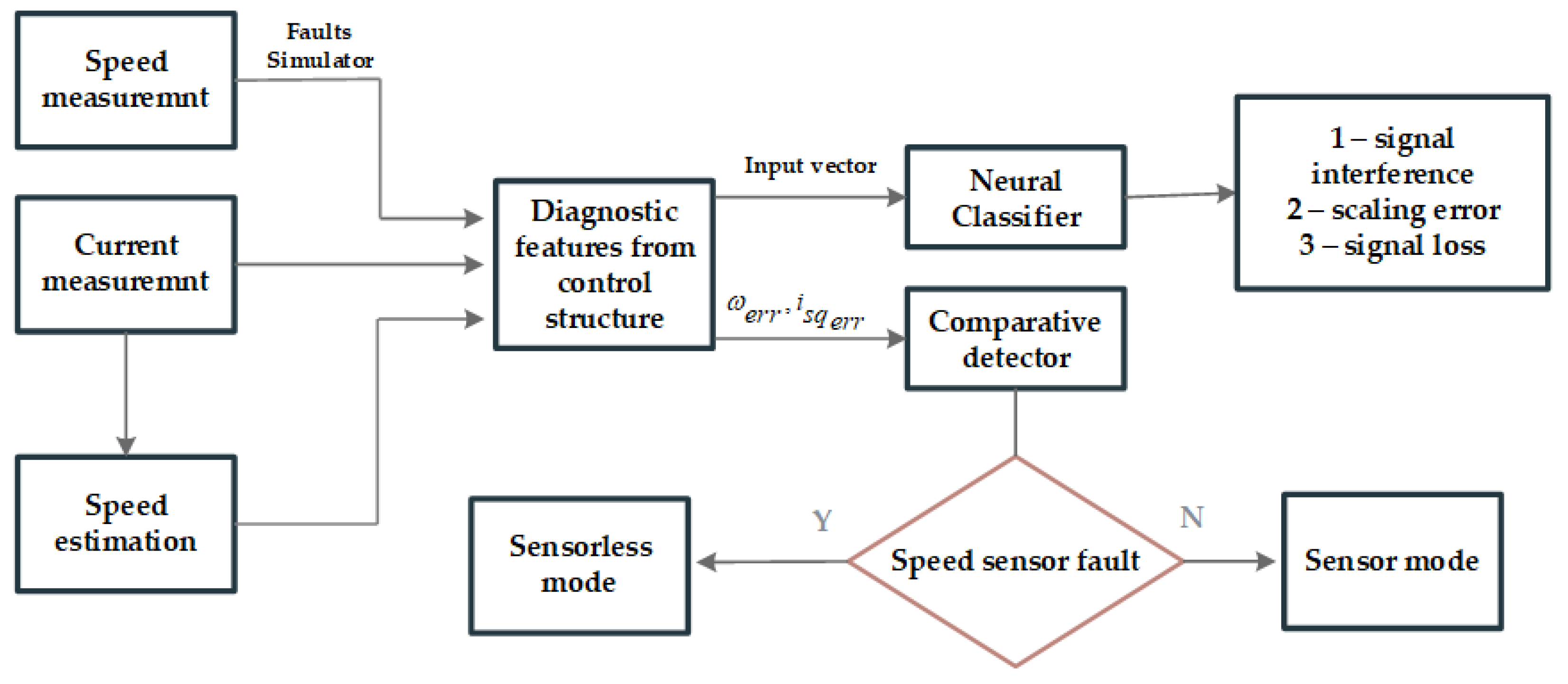
This chapter presents experimental results obtained from offline and online detection. The first stage of developing the classifier was to perform measurements and prepare the network input vector (training and testing data). In the next step, an appropriate structure was selected 23-10-1, and training of neural networks and an analysis of effectiveness in offline classification were carried out. In the last stage, the trained network was implemented on a laboratory set-up, and online classification was carried out. In the proposed solution, the system is switched to sensorless mode based on the response of the comparative detector. The neural classifier, on the other hand, is only an indicator of the failure type. A flowchart of the described solution is presented in
Figure 8.
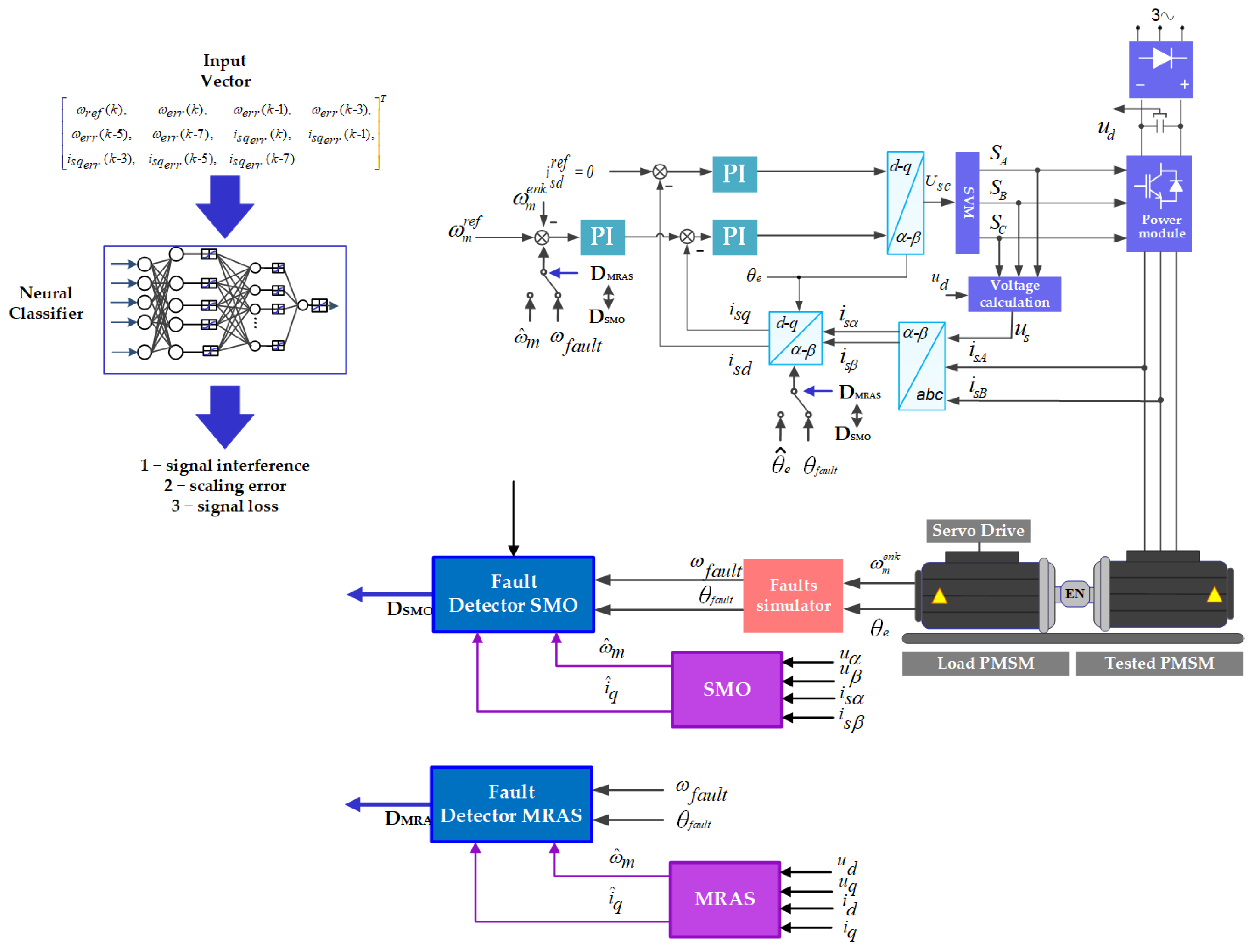
The complete control structure of the drive system with the detector and neural classifier is shown in
Figure 9. Faults during the research were simulated in a software manner. The results are presented per unit.
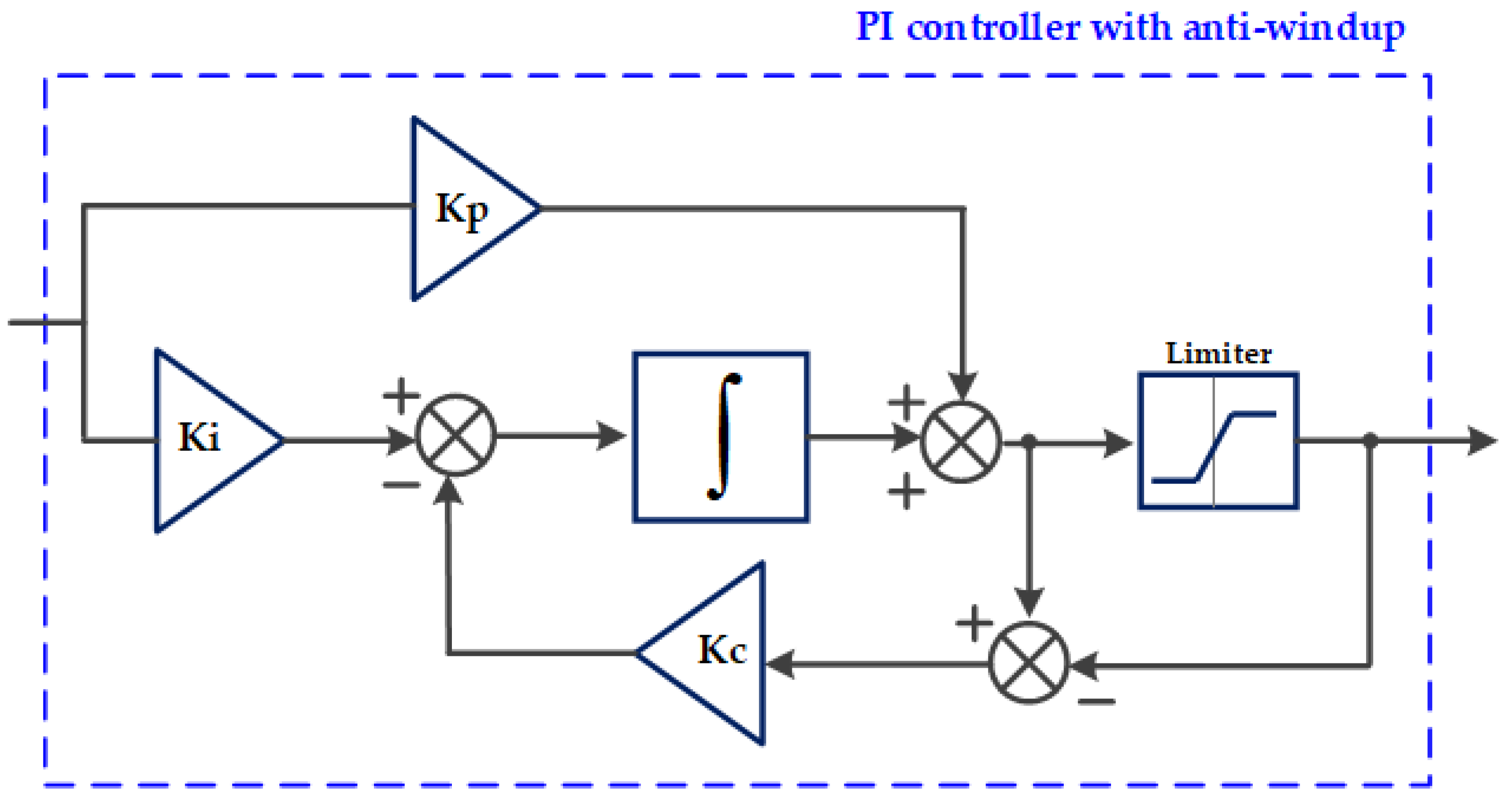
In the research, the same type of PI regulator with anti-windup with a correction parameter was used to control the speed and currents in the d and q axes in the rotor frame. The block diagram of the applied system is shown in
Figure 10.
The classifier effectiveness has been shown using confusion matrixes (
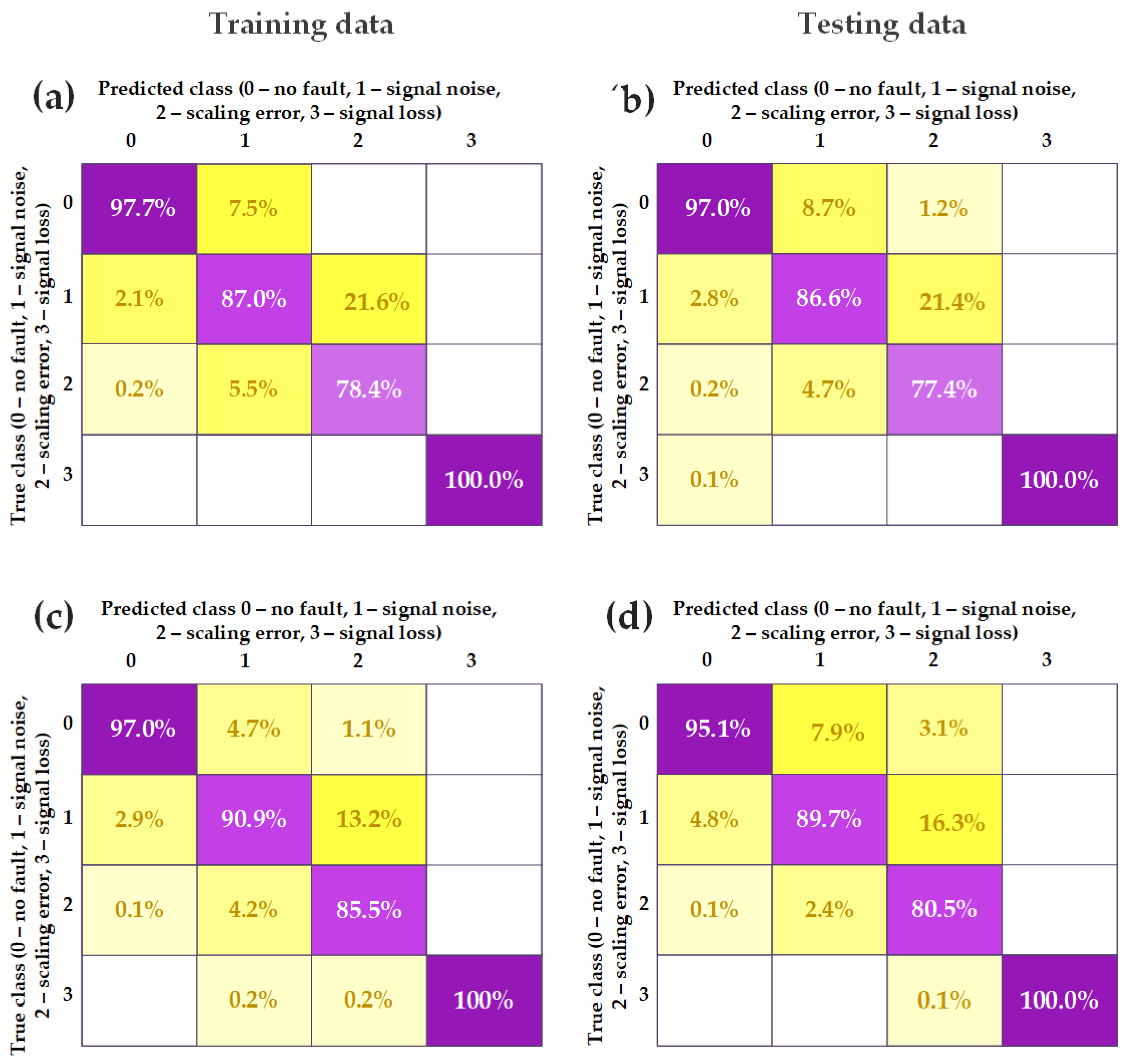
Figure 11). Confusion matrixes are presented for neural classifier performance analysis obtained by offline classification. The exact parameters of the training and testing vectors are presented in
Table 3. Based on the values presented in the table, it can be concluded that the network was tested for both interpolation and extrapolation.
Based on
Figure 11, it can be concluded that the SMO-based approach allows for higher efficiency. In the case of both classifiers, both for training and test data, 100% classification of signal loss was obtained. Most errors occur with scaling errors. This is largely because, for low speeds, the difference between the estimated and the measured speed is small. The detectability of this error increases with increasing speed. An important conclusion that can be drawn from the presented results is that the scaling error and signal interference are detected with high efficiency, but the network makes mistakes in distinguishing them. This is also confirmed by the high efficiency of indicating the operation without damage. The analysis of the influence of the input vector signals on the classifier output is presented using correlations in
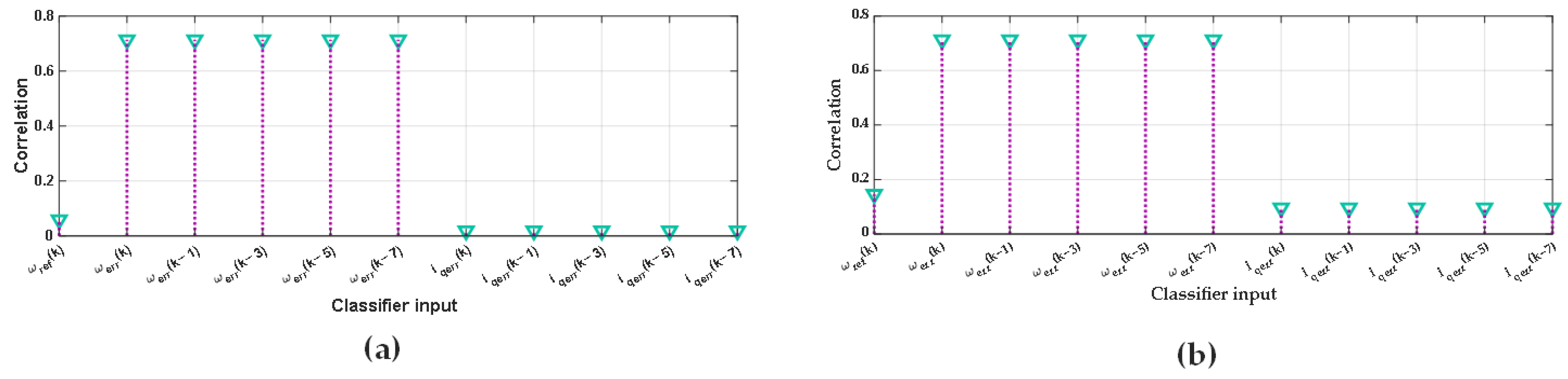
Figure 12. In the case of both classifiers, the inputs related to the speed are definitely more important. The q-axis current in rotor frame inputs is an auxiliary symptom. The same applies to the reference speed.
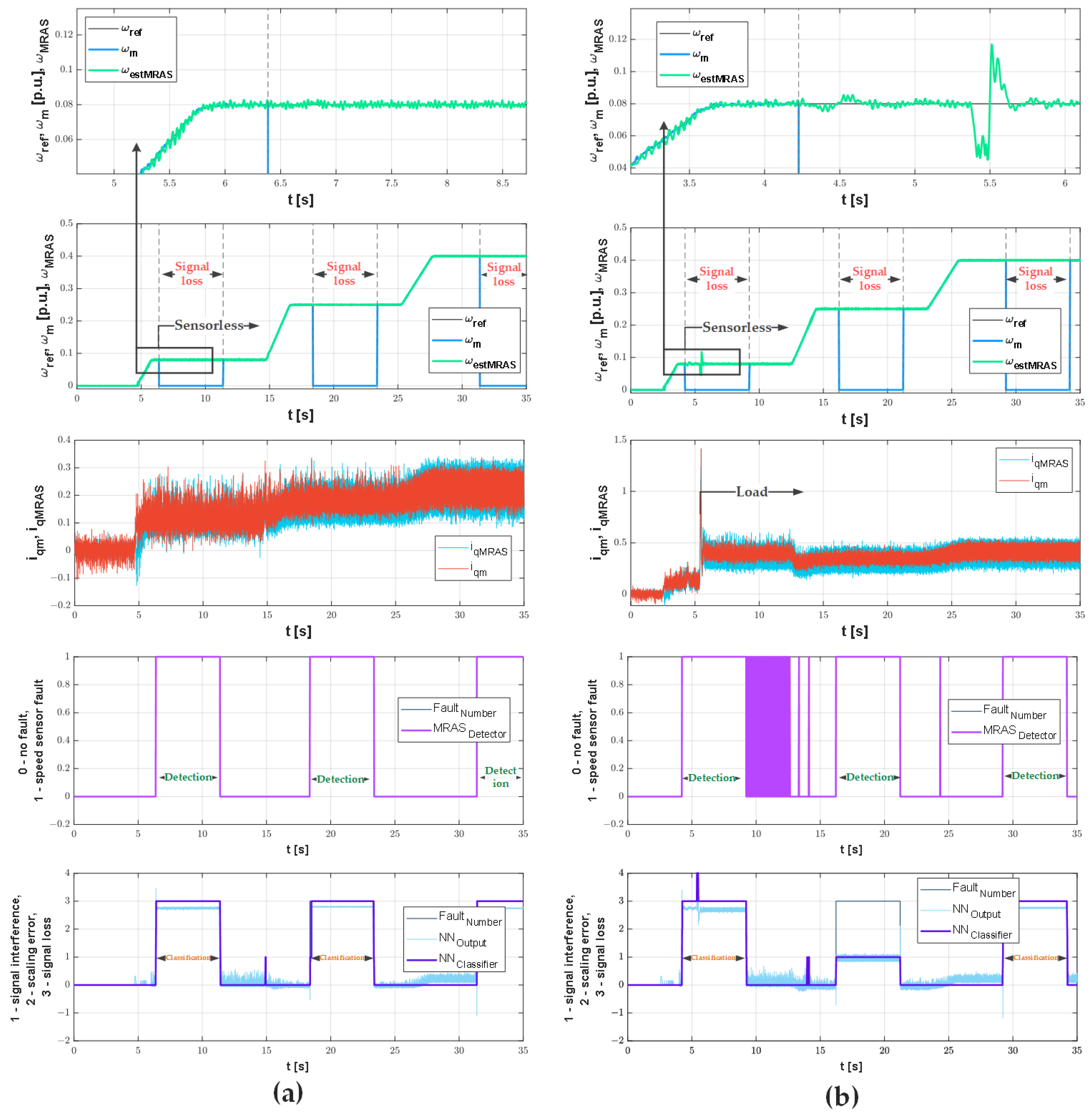
The following results show sample transients for online detection and classification. First, the signal loss with and without load for different speeds for the classifier based on MRAS (
Figure 13) is presented. In the neural classifier transients, the raw output of the neural network is shown
NNOutput—and the output of the classifier, which is the rounded value of five samples of the network output—
NNClassifier.
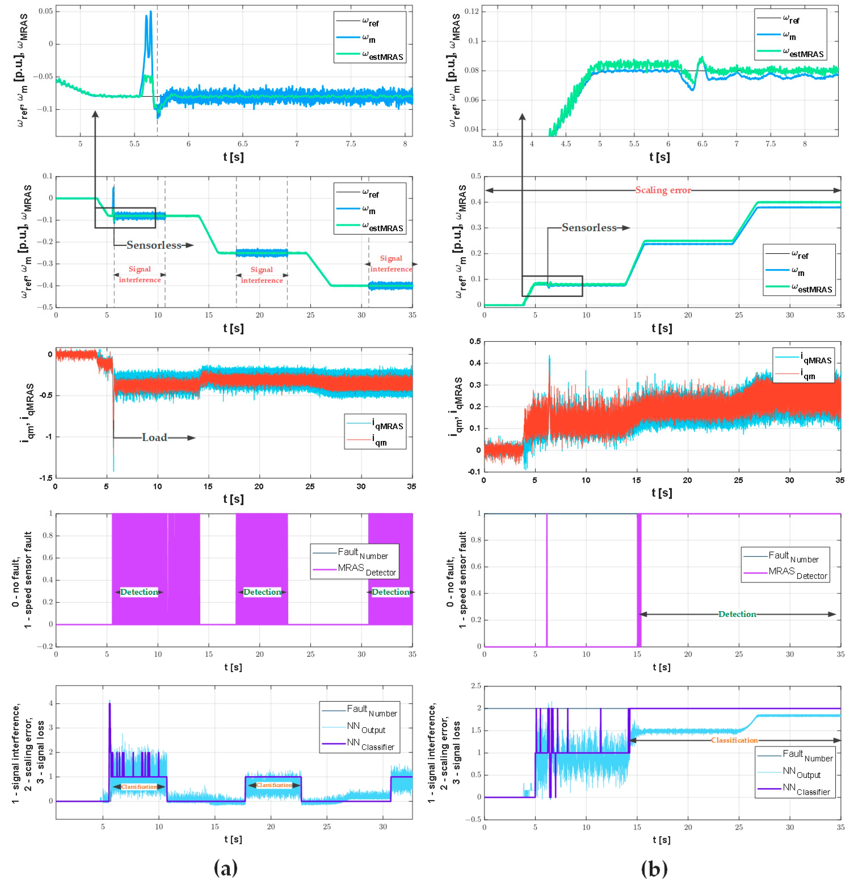
Switching on the load degrades the properties of both the detector and the classifier. There are false positives and misclassification. The moment of switching on the load causes additional noise that has been misclassified. As the operating speed increases, the detection and classification systems improve, and the influence of motor load decreases. Motor load also reduces the accuracy of the current estimation in the iq axis. The results obtained for less significant damages, scaling error, and signal interference are shown in
Figure 14. In this case, a significant advantage of the neural classifier over the comparative detector can be noticed. Signal interferences are classified using a constant signal, not pulses. On the other hand, the scaling error, which is switched on from the start of the system operation, is detected only after reaching the speed about
.
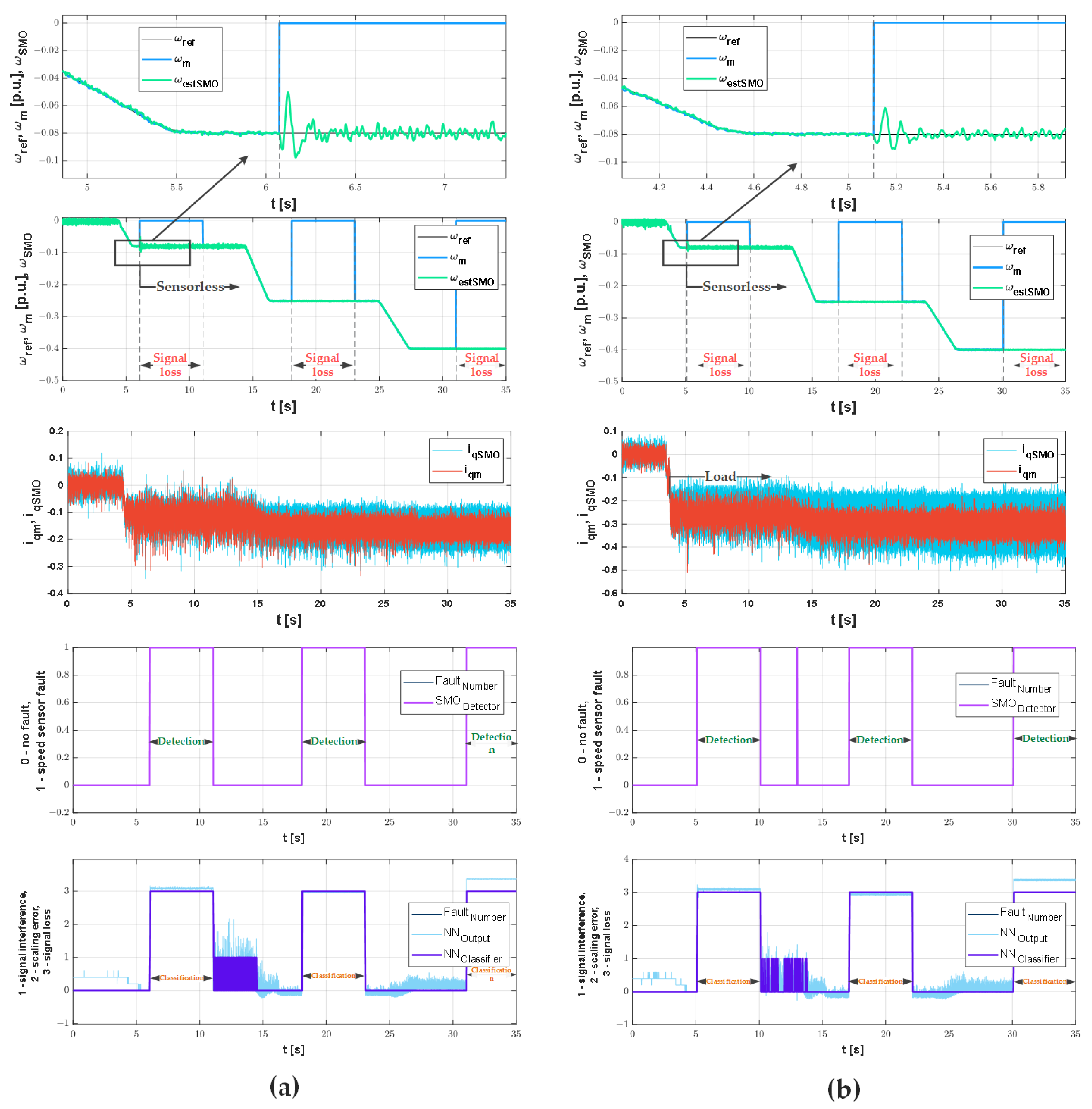
The next two figures show the online classification based on the SMO. They confirm the higher efficiency obtained for this classifier. During signal loss (
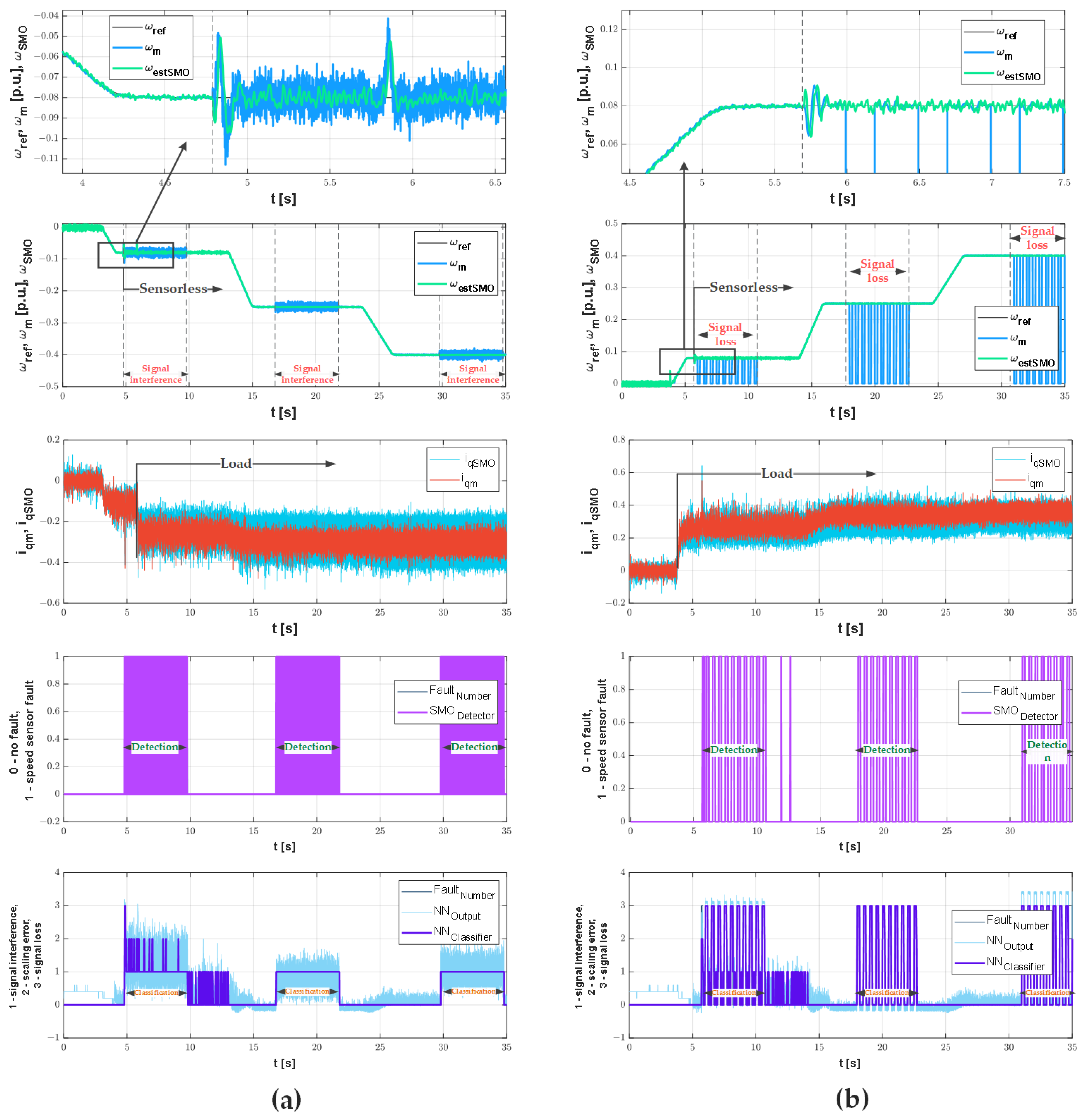
Figure 15), both the detector and the classifier almost do not make errors. The load also slightly affects the efficiency of the system. In this case, too, the increase in speed improves the performance of the system. This is especially important for the SMO-based classifier because the version used in the article does not work correctly for the lowest speeds. Motor start in sensorless mode, unlike MRAS, is impossible as it requires additional systems. Signal interferences are detected with high efficiency, while the quick detection of cyclic signal losses shows the dynamics of the detector’s operation (
Figure 16). In addition, the advantage of the SMO-based system is a much smaller impact of the motor load on the correct classification.
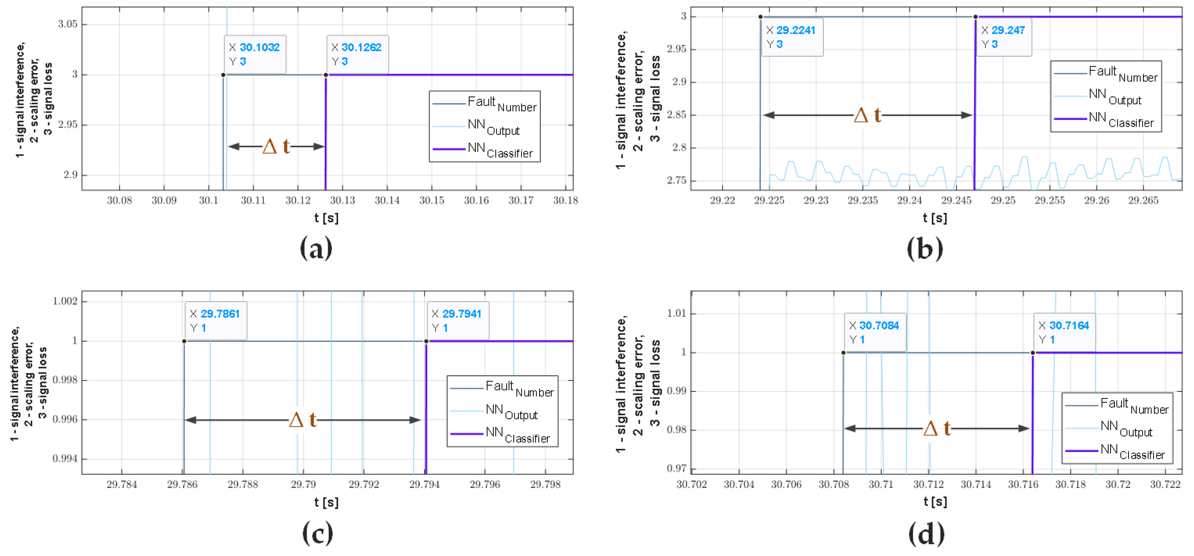
An important element of FTC systems is also the failure detection and classification time. Failure detection with a comparison detector in both cases—SMO and MRAS—is less than 0.0005 s. This time is not observable on the transients because every fifth sample was collected, and the sampling time was 0.0001. Whereas the classification times obtained for the testing vector under motor load conditions are presented in
Table 4. Due to the method of data acquisition, the times presented in the table are approximate values.
Classification times for both types of classifiers are at a similar level. Classification times are, in most cases, less than 30 ms. It can also be inferred from the table that the detection time decreases with increasing speed. Example Transients showing the time of occurrence and classification of failures are shown in
Figure 17.
5. Conclusions
The paper describes the possibilities of detection and classification of speed sensor faults in the PMSM control system based on MRAS, SMO, and neural networks. One of the estimators is responsible for the detection, while the neural structure is responsible for the classification. Detection is fast enough for the system to switch to sensorless mode even when the signal is lost. This made it possible to conduct experimental research. This is considered to be a significant advantage of the work, as most of the articles in the literature show only simulation results. Damage classification is an additional element of the monitoring system. It allows for obtaining practical information about the damage: the need to replace and change the scaling or calibration parameters. It can also indicate that the measured signal is disturbed. In advanced machine condition monitoring systems, such solutions are sought. Research shows a clear advantage of the SMO-based system. The estimation of the speed using the SMO system is more accurate. The obtained results also show the importance of conducting further research in the field of speed sensor faults classification with the use of neural networks. The next step in the authors’ research will be the use of deep learning methods.
Author Contributions
Conceptualization, M.D. and K.J.; methodology, M.D. and K.J.; software, K.J. and V.P.; validation, M.D. and K.J.; formal analysis, M.D., K.J., V.P. and K.K.; investigation, M.D. and K.J.; resources, M.D. and K.J.; data curation, K.J.; writing—original draft preparation, K.J.; writing—review and editing, M.D., V.P. and K.K.; visualization, K.J.; supervision, M.D.; project administration, M.D.; funding acquisition, M.D. All authors have read and agreed to the published version of the manuscript.
Funding
This work was supported by the Scientific Grant Agency of the Ministry of Education of the Slovak Republic under the project VEGA 1/0363/23 and from the statutory funds of the Department of Electrical Machines, Drives and Measurements, Wroclaw University of Science and Technology.
Institutional Review Board Statement
Not applicable.
Informed Consent Statement
Not applicable.
Data Availability Statement
Not applicable.
Conflicts of Interest
The authors declare no conflict of interest.
References
- Li, L.; Ding, S.X.; Luo, H.; Peng, K.; Yang, Y. Performance-Based Fault-Tolerant Control Approaches for Industrial Processes with Multiplicative Faults. IEEE Trans. Ind. Inform. 2020, 16, 4759–4768. [Google Scholar] [CrossRef]
- Bouakoura, M.; Naăźt-Saăźd, N.; Naăźt-Saăźd, M.-S. Speed Sensor Faults Diagnosis in an Induction Motor Vector Controlled Drive. Acta Electrotech. Inform. 2017, 17, 49–51. [Google Scholar] [CrossRef]
- Bensalem, Y.; Kouzou, A.; Abbassi, R.; Jerbi, H.; Kennel, R.; Abdelrahem, M. Sliding-Mode-Based Current and Speed Sensors Fault Diagnosis for Five-Phase PMSM. Energies 2022, 15, 71. [Google Scholar] [CrossRef]
- Hezzi, A.; Abdelkrim, M.N.; Ben Elghali, S. Robust Active Fault Tolerant Control for Five-Phase PMSM against Speed Sensor Failures. In Proceedings of the 2021 18th International Multi-Conference on Systems, Signals & Devices (SSD), Monastir, Tunisia, 22–25 March 2021; pp. 575–579. [Google Scholar] [CrossRef]
- Jlassi, I.; Cardoso, A.J.M. A single fault diagnostics approach for power switches, speed sensors and current sensors in regenerative PMSM drives. In Proceedings of the 2017 IEEE 11th International Symposium on Diagnostics for Electrical Machines, Power Electronics and Drives (SDEMPED), Tinos, Greece, 29 August–1 September 2017; pp. 366–372. [Google Scholar] [CrossRef]
- Xia, J.; Guo, Y.; Dai, B.; Zhang, X. Sensor fault tolerant control method for electric traction PWM rectifier using sliding mode observer. In Proceedings of the 2016 19th International Conference on Electrical Machines and Systems (ICEMS), Chiba, Japan, 13–16 November 2016; pp. 1–6. [Google Scholar]
- Kommuri, S.K.; Defoort, M.; Karimi, H.R.; Veluvolu, K.C. A Robust Observer-Based Sensor Fault-Tolerant Control for PMSM in Electric Vehicles. IEEE Trans. Ind. Electron. 2016, 63, 7671–7681. [Google Scholar] [CrossRef]
- Nicola, M.; Nicola, C.-I. Sensorless Control of PMSM using SMC and Sensor Fault Detection Observer. In Proceedings of the 2021 18th International Multi-Conference on Systems, Signals & Devices (SSD), Monastir, Tunisia, 22–25 March 2021; pp. 518–525. [Google Scholar] [CrossRef]
- Bourogaoui, M.; Jlassi, I.; El Khil, S.K.; Sethom, H.B.A. An effective encoder fault detection in PMSM drives at different speed ranges. In Proceedings of the 2015 IEEE 10th International Symposium on Diagnostics for Electrical Machines, Power Electronics and Drives (SDEMPED), Guarda, Portugal, 1–4 September 2015; pp. 90–96. [Google Scholar] [CrossRef]
- Odgaard, P.F.; Stoustrup, J. Unknown input observer based detection of sensor faults in a wind turbine. In Proceedings of the 2010 IEEE International Conference on Control Applications, Yokohama, Japan, 8–10 September 2010; pp. 310–315. [Google Scholar] [CrossRef]
- Salem, M.H.; Bensalem, Y.; Abdelkrim, M.N. A Speed Sensor Fault Tolerant Control for a Permanent Magnet Synchronous Motor. In Proceedings of the 2020 17th International Multi-Conference on Systems, Signals & Devices (SSD), Monastir, Tunisia, 20–23 July 2020; pp. 290–295. [Google Scholar] [CrossRef]
- Zhao, H.; Luo, P.; Wang, N.; Zheng, Z.; Wang, Y. Fuzzy logic control of the fault-tolerant PMSM servo system based on MRAS observer. In Proceedings of the 2018 Chinese Control and Decision Conference (CCDC), Shenyang, China, 9–11 June 2018; pp. 1812–1817. [Google Scholar] [CrossRef]
- Ben Slimen, S.; Bourogaoui, M.; Sethom, H.B.A. A New Approach for Effective Position/Speed Sensor Fault Detection in PMSM Drives. In Electrimacs Lecture Notes in Electrical Engineering; Zamboni, W., Petrone, G., Eds.; Springer: Cham, Switzerland, 2019; Volume 615. [Google Scholar] [CrossRef]
- Dybkowski, M. Wybrane detektory uszkodzeń czujnika prędkości obrotowej dla napędu wektorowego z silnikiem indukcyjnym. Przegląd Elektrotechniczny 2016, 1, 87–93. [Google Scholar] [CrossRef]
- Pietrzak, P.; Wolkiewicz, M.; Orlowska-Kowalska, T. PMSM Stator Winding Fault Detection and Classification Based on Bispectrum Analysis and Convolutional Neural Network. IEEE Trans. Ind. Electron. 2022, 70, 5192–5202. [Google Scholar] [CrossRef]
- Skowron, M.; Orlowska-Kowalska, T.; Kowalski, C.T. Diagnosis of Stator Winding and Permanent Magnet Faults of PMSM Drive Using Shallow Neural Networks. Electronics 2023, 12, 1068. [Google Scholar] [CrossRef]
- Ewert, P.; Orlowska-Kowalska, T.; Jankowska, K. Effectiveness Analysis of PMSM Motor Rolling Bearing Fault Detectors Based on Vibration Analysis and Shallow Neural Networks. Energies 2021, 14, 712. [Google Scholar] [CrossRef]
- Guedidi, A.; Guettaf, A.; Cardoso, A.J.M.; Laala, W.; Arif, A. Bearing Faults Classification Based on Variational Mode Decomposition and Artificial Neural Network. In Proceedings of the 2019 IEEE 12th International Symposium on Diagnostics for Electrical Machines, Power Electronics and Drives (SDEMPED), Toulouse, France, 27–30 August 2019; pp. 391–397. [Google Scholar] [CrossRef]
- Dybkowski, M.; Klimkowski, K. Artificial Neural Network Application for Current Sensors Fault Detection in the Vector Controlled Induction Motor Drive. Sensors 2019, 19, 571. [Google Scholar] [CrossRef] [PubMed] [Green Version]
- Skowron, M.; Teler, K.; Adamczyk, M.; Orlowska-Kowalska, T. Classification of Single Current Sensor Failures in Fault-Tolerant Induction Motor Drive Using Neural Network Approach. Energies 2022, 15, 6646. [Google Scholar] [CrossRef]
- Jankowska, K.; Dybkowski, M. Experimental Analysis of the Current Sensor Fault Detection Mechanism Based on Neural Networks in the PMSM Drive System. Electronics 2023, 12, 1170. [Google Scholar] [CrossRef]
- Qin, J.; Du, J. Minimum-learning-parameter-based adaptive finite-time trajectory tracking event-triggered control for underactuated surface vessels with parametric uncertainties. Ocean. Eng. 2023, 271, 113634. [Google Scholar] [CrossRef]
- Bai, H.; Yu, B.; Gu, W. Research on Position Sensorless Control of RDT Motor Based on Improved SMO with Continuous Hyperbolic Tangent Function and Improved Feedforward PLL. J. Mar. Sci. Eng. 2023, 11, 642. [Google Scholar] [CrossRef]
- Qin, J.; Du, J.; Li, J. Adaptive Finite-Time Trajectory Tracking Event-Triggered Control Scheme for Underactuated Surface Vessels Subject to Input Saturation. In IEEE Transactions on Intelligent Transportation Systems; IEEE: Piscataway, NJ, USA, 2023. [Google Scholar] [CrossRef]
- Utkin, V.; Guldner, J.; Shi, J. Sliding Mode Control in Electromechanical Systems, 1st ed.; Taylor & Francis: London, UK, 1999. [Google Scholar]
- Kyslan, K.; Petro, V.; Bober, P.; Šlapák, V.; Ďurovský, F.; Dybkowski, M.; Hric, M. A Comparative Study and Optimization of Switching Functions for Sliding-Mode Observer in Sensorless Control of PMSM. Energies 2022, 15, 2689. [Google Scholar] [CrossRef]
Figure 1.
Photos of the experimental set-up.
Figure 1.
Photos of the experimental set-up.
Figure 2.
Model reference adaptive system used in research structure, where estimated is electrical motor position.
Figure 2.
Model reference adaptive system used in research structure, where estimated is electrical motor position.
Figure 3.
Transients of speed, current in q axis, and rotor position measured and estimated by MRAS in sensor (a) and sensorless (b) mode.
Figure 3.
Transients of speed, current in q axis, and rotor position measured and estimated by MRAS in sensor (a) and sensorless (b) mode.
Figure 4.
Sensorless startup with model reference adaptive system.
Figure 4.
Sensorless startup with model reference adaptive system.
Figure 5.
Block diagram of the reduced SMO used in the research.
Figure 5.
Block diagram of the reduced SMO used in the research.
Figure 6.
Transients of speed, current in q axis, and rotor position measured and estimated by SMO in sensor (a) and sensorless (b) mode.
Figure 6.
Transients of speed, current in q axis, and rotor position measured and estimated by SMO in sensor (a) and sensorless (b) mode.
Figure 7.
Transients of measured and estimated speed error with the use of MRAS (a) and SMO (b) in no load conditions.
Figure 7.
Transients of measured and estimated speed error with the use of MRAS (a) and SMO (b) in no load conditions.
Figure 8.
Flowchart of detection, classification, and compensation system presented in the article.
Figure 8.
Flowchart of detection, classification, and compensation system presented in the article.
Figure 9.
Control structure, including observer-based detectors and a neural classifier.
Figure 9.
Control structure, including observer-based detectors and a neural classifier.
Figure 10.
Control structure, including observer-based detectors and a neural classifier.
Figure 10.
Control structure, including observer-based detectors and a neural classifier.
Figure 11.
Confusion matrixes with effectiveness obtained by MRAS-based classifier for training (a) and testing data (b) and SMO-based classifier for training (c) and testing data (d).
Figure 11.
Confusion matrixes with effectiveness obtained by MRAS-based classifier for training (a) and testing data (b) and SMO-based classifier for training (c) and testing data (d).
Figure 12.
Correlation values between input vector elements and output vector in classifier based on MRAS (a) and SMO (b).
Figure 12.
Correlation values between input vector elements and output vector in classifier based on MRAS (a) and SMO (b).
Figure 13.
Speed, MRAS detector, and neural classifier transients during signal loss without motor load (a) and with motor load 0.15TN (b).
Figure 13.
Speed, MRAS detector, and neural classifier transients during signal loss without motor load (a) and with motor load 0.15TN (b).
Figure 14.
Speed, MRAS detector, and neural classifier transients during signal interference with motor load 0.15TN (a) and scaling error without motor load (b).
Figure 14.
Speed, MRAS detector, and neural classifier transients during signal interference with motor load 0.15TN (a) and scaling error without motor load (b).
Figure 15.
Speed, SMO detector, and neural classifier transients during signal loss without motor load (a) and with motor load 0.15TN (b).
Figure 15.
Speed, SMO detector, and neural classifier transients during signal loss without motor load (a) and with motor load 0.15TN (b).
Figure 16.
Speed, SMO detector, and neural classifier transients with motor load 0.15TN during signal interference (a) and cyclic signal loss (b).
Figure 16.
Speed, SMO detector, and neural classifier transients with motor load 0.15TN during signal interference (a) and cyclic signal loss (b).
Figure 17.
Failure classification times for signal loss based on SMO (a) and MRAS (b) and signal interference based on SMO (c) and MRAS (d).
Figure 17.
Failure classification times for signal loss based on SMO (a) and MRAS (b) and signal interference based on SMO (c) and MRAS (d).
Table 1.
Parameters of tested motor.
Table 1.
Parameters of tested motor.
| PN [kW] | Pp [-] | nN [rpm] | TN [Nm] | IN [A] | J [kg·m2] | RS [Ω] |
|---|
| 0.894 | 4 | 6200 | 1.4 | 1.9 | 0.000039 | 4.6615 |
Table 2.
Description of individual NN classifier inputs.
Table 2.
Description of individual NN classifier inputs.
| Input | Value MRAS | Value SMO | Description |
|---|
| | | Reference speed value. |
| | | Error between measured and estimated speed value in actual sample. |
| , , , | ,
,
,
| ,
,
,
| Error between measured and estimated speed value in previous samples. |
| | | Error between measured and estimated q-axis current value in actual sample. |
| , , , | ,
,
,
| ,
,
,
| Error between measured and estimated q-axis current value in previous samples. |
Table 3.
Parameters of training and testing vectors in experimental studies.
Table 3.
Parameters of training and testing vectors in experimental studies.
| Feature | Training Data | Testing Data |
|---|
| Number of samples | 1,260,162 | 840,096 |
| Speed values | +/−0.1ωref, +/−0.2ωref, +/−0.35ωref | +/−0.08ωref, +/−0.25ωref, +/−0.4ωref |
| Load Values | 0.1TN, 0.2TN | 0.15TN |
Table 4.
Classification times obtained in motor load conditions.
Table 4.
Classification times obtained in motor load conditions.
| | MRAS | SMO |
|---|
| Speed | 0.08ωref | 0.25ωref | 0.4ωref | 0.08ωref | 0.25ωref | 0.4ωref |
| Signal loss | 21 ms | 11 ms | 23 ms | 28 ms | 34 ms | 23 ms |
Signal
interference | 29 ms | 13 ms | 8 ms | 23 ms | 13 ms | 8 ms |
| Disclaimer/Publisher’s Note: The statements, opinions and data contained in all publications are solely those of the individual author(s) and contributor(s) and not of MDPI and/or the editor(s). MDPI and/or the editor(s) disclaim responsibility for any injury to people or property resulting from any ideas, methods, instructions or products referred to in the content. |
© 2023 by the authors. Licensee MDPI, Basel, Switzerland. This article is an open access article distributed under the terms and conditions of the Creative Commons Attribution (CC BY) license (https://creativecommons.org/licenses/by/4.0/).


