Soil-Surface-Image-Feature-Based Rapid Prediction of Soil Water Content and Bulk Density Using a Deep Neural Network

Abstract

This study aimed to develop a deep neural network model for predicting the soil water content and bulk density of soil based on features extracted from in situ soil surface images. Soil surface images were acquired using a Canon EOS 100d camera. The camera was installed in the vertical direction above the soil surface layer. To maintain uniform illumination conditions, a dark room and LED lighting were utilized. Following the acquisition of soil surface images, soil samples were collected using a metal cylinder to obtain measurements of soil water content and bulk density. Various features were extracted from the images, including color, texture, and shape features, and used as inputs for both a multiple regression analysis and a deep neural network model. The results show that the deep neural network regression model can predict soil water content and bulk density with root mean squared error of 1.52% and 0.78 kN/m³. The deep neural network model outperformed the multiple regression analysis, achieving a high accuracy for predicting both soil water content and bulk density. These findings suggest that in situ soil surface images, combined with deep learning techniques, can provide a fast and reliable method for predicting important soil properties.

1. Introduction

Climate change is having a significant impact on water resources worldwide, which in turn is affecting the agricultural environment. In this context, identifying the characteristics of soil in the field has become increasingly important to predict changes in global water resources. The infiltration rate and evapotranspiration of the surface layer can vary depending on the change in soil water content and bulk density. Since topsoil properties tend to change greatly over time, it is important to rapidly identify topsoil properties in terms of the global hydrologic cycle [1].

The need for soil characterization is further increasing due to the expansion of smart farms, which require an autonomous management system for large-scale agricultural land [2]. Nowadays, various soil property prediction systems have been established, ranging from wide-scale global monitoring using remote sensing to the precise monitoring of points using IoT sensors [3,4]. Additionally, precision agriculture, driven by smart farms, requires the development of various sensors for more precise soil management [5]. Therefore, it is crucial to develop the rapid and precise identification of soil characteristics for both large-scale factory farming and small-scale precision agriculture.

Soil property prediction methods can be broadly categorized into experiments, sensors, and feeling tests. Experiments are the most reliable method, but are time consuming and costly [6]. Sensors collectively refer to devices that can collect information, and there are various sensors on the market, such as permittivity sensors for predicting soil moisture, pressure gauges, and electrical resistivity tomography for ground investigations [7,8,9]. Optical equipment, such as satellites and digital cameras, can also be classified as sensors because they collect information about an object’s wavelength or color. Sensory tests may appear somewhat irrational and unscientific, but they have been used for a long time and are still valuable in predicting soil properties. In feeling tests, the texture, color, and scent are used to identify soil properties. The Munsell chart is widely used for classifying forest soil and can be regarded as an example of a color-based feeling test [10]. In particular, soil texture can be predicted with a high level of accuracy through feeling tests [11,12,13]. Soil water content and bulk density can also be roughly estimated through feeling tests, but quantitative values can be difficult to obtain [14,15].

Digital image processing (DIP) is a technique used to extract useful information from digital images. This can be regarded as an extension of the feeling test using vision, in that information is obtained based on the distribution of color information present in a digital image [16]. Unlike qualitative and empirical feeling tests, DIP can provide quantitative and repeatable information [17,18]. From digital images of soil, various information such as color, texture, and the distribution of soil particles and voids can be obtained [19,20].

Deep neural network (DNN) models are useful tools for analyzing complex relationships between input and output variables. These models can extract important features from large and complicated datasets, enabling them to understand the data on a higher level [21,22]. DNN models are especially effective for analyzing datasets with nonlinear relationships between input and output variables. Furthermore, DNN models can be generalized to new data well, making them suitable for accurate predictions on previously unseen samples. There have been various attempts at using various deep learning models including DNN to predict soil properties. For instance, Islam et al. [23] employed a total of 46 parameters in their model to predict crop selection and yield. Other studies have shown that it is possible to predict soil texture from images by extracting relevant features, as exemplified by Kumar et al. [24] and Zhao et al. [20]. Similarly, Wu et al. [25] used a convolutional neural network to predict permeability based on images. These examples illustrate the potential of DNN models in analyzing complex relationships between input and output variables for a wide range of applications. Therefore, using a DNN regression model is appropriate for predicting soil water content and bulk density based on the extracted various features from soil surface images.

The objectives of this study were to investigate the potential of a DNN regression model using in situ soil surface images for predicting soil water content and bulk density. A digital image acquisition device was fabricated to acquire in situ soil surface images under various soil water content and bulk density conditions. Through digital image processing, features that can express color, texture, and shape were extracted from soil surface images and used as input parameters for DNN regression models. Multiple regression analysis was performed to compare the performance with the DNN regression models.

2. Materials and Methods

2.1. Soil Sampling and Measurement of Water Content and Bulk Density

Table 1. Soil water content and bulk density of in situ soil samples.

Sampling Point	Texture	Location	Number of Images	Water Content (%)				Bulk Density (kN/m3)
				Max	Mean	Min	Range	Max	Mean	Min	Range
A	SiL	37°16′09.7″ N 126°59′18.9″ E	128	17.8	9.2	1.2	16.6	12.7	10.9	7.8	4.9
B	SL	37°16′15.6″ N 126°59′15.9″ E	144	22.3	12.7	4.6	17.8	14.7	11.2	8.3	6.4
C	LS	37°27′28.5″ N 126°56′52.6″ E	96	21.6	14.7	9.6	12.0	16.2	12.4	9.1	7.1

presents a summary of the properties of in situ soil samples used in this study, along with the measurement results of two target variables: water content and bulk density. This study selected three different locations, denoted as A, B, and C, each with soils of different textures: silt loam (SiL), sandy loam (SL), and loamy sand (LS), respectively.

To obtain data on the soil surface, 128, 144, and 96 images were taken at points A, B, and C, respectively. Following the image capture, soil sampling was conducted using a metal cylinder with a diameter of 50 mm and a height of 51 mm. To ensure comprehensive coverage of the area of the soil surface image, four samples were collected at each location in a 2 × 2 arrangement using four metal cylinders. Therefore, 512, 576, and 384 soil samples were collected at points A, B, and C, respectively. The WC and BD for each location were computed by taking the average of four samples. Accordingly, there existed 128, 144, and 96 data for WC and BD at points A, B, and C, correspondingly, matching the number of digital images. WC and BD were determined by Equations (1) and (2), respectively.

$$\mathrm{WC}\left(\%\right)=\frac{W_w}{W_s}\times 100=\frac{W_2-W_3}{W_3-W_1}\times 100$$

(1)

$$\mathrm{BD}\left(\mathrm{kN}/{\mathrm{m}}^3\right)=\frac{W_s}{V_s}$$

(2)

where $W_w$ is the weight of water, $W_s$ is the weight of dry soil, $W_1$ is the weight of the container (metal cylinder), $W_2$ is the weight of the container with wet soil, $W_3$ is the weight of the container with dry soil and $V_s$ is the volume of soil (same as the volume of the container). To measure the weight of dry soil, the soil samples were completely dried at 110 ± 5 °C for 24 h using a drying oven (Changshin Science C-DOD3, Seoul, Republic of Korea). WC ranged from a low of 1.2% to a high of 22.3%, ranging from very dry soil to moist soil. BD also includes loose to dense soils, from a minimum of 7.8 kN/m³ to a maximum of 16.2 kN/m³.

2.2. Acquisition of Soil Surface Images

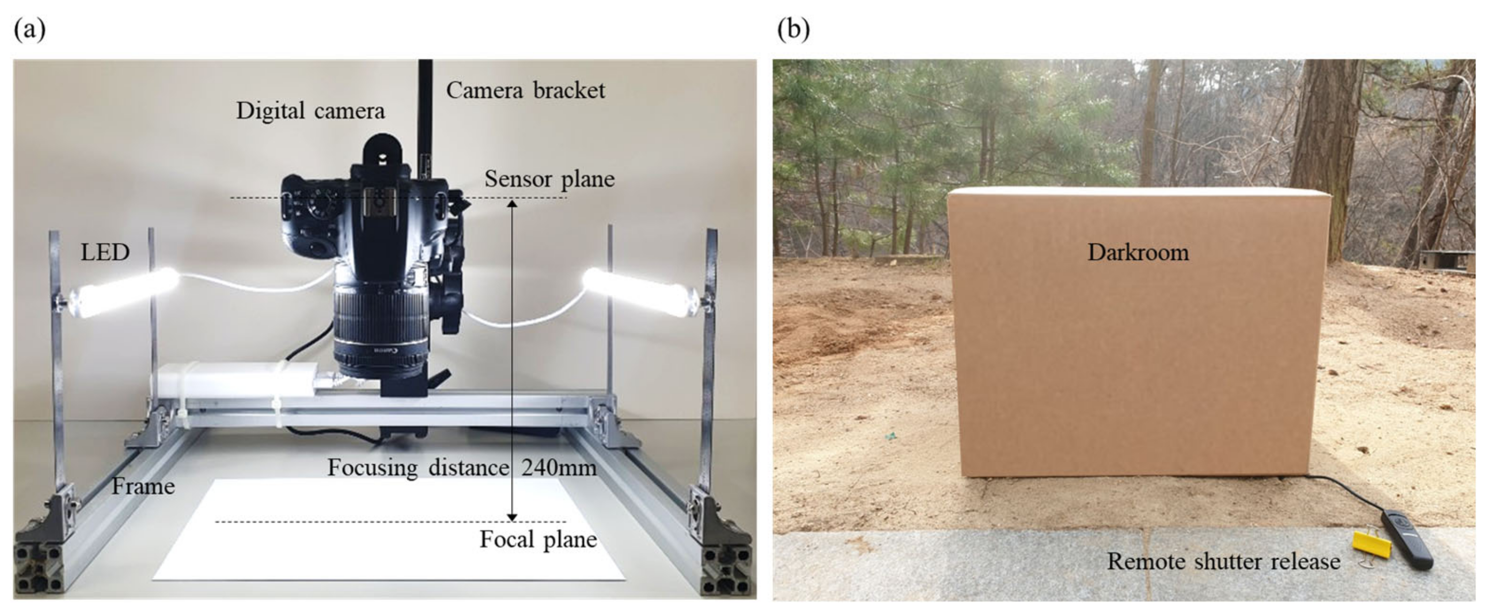
Figure 1 shows a camera setup used for acquiring soil surface images in the field. The Canon EOS 100d camera model was used with specific settings, including a 35 mm focal length, 1/4 sec exposure time, 9.0 aperture, and ISO sensitivity 100. The camera was mounted vertically using a frame and camera bracket, with a focusing distance of 240 mm. The size of the digital image was 5184 × 3456 pixels, representing an area of 93.3 mm × 62.2 mm. Proper lighting conditions are crucial when capturing in situ images. Changes in lighting conditions can alter the color distribution of the soil surface images, which was a critical aspect of this study. Therefore, the lighting was carefully selected after evaluating natural light, camera lighting, and LED lighting, ultimately choosing LED lights that provide even illumination. To ensure consistent lighting conditions, a box-shaped darkroom was constructed to prevent external light interference. In addition, a remote shutter release was used to prevent shaking of the camera during shooting.

2.3. Features in Soil Surface Image

In this study, we extracted various features from soil surface images for use in a DNN model and multiple regression analysis. Soil color is an effective factor in predicting soil characteristics [26]. Digital images are composed of pixels, each representing a point with color information. The most commonly used color system is RGB, which stands for red, green, and blue, and represents the amount of each color in each pixel. However, since each component of RGB is highly correlated with each other, it is difficult to intuitively infer the color of an image by looking at RGB values only. Therefore, color systems composed of features representing different characteristics have been proposed. One such system is HSV, which stands for hue, saturation, and value. Hue refers to the dominant color, with red at 0 degrees, green at 120 degrees, and blue at 240 degrees. Saturation means the purity of color and value refers to the brightness of color. These three features, hue, saturation and value, were extracted from color images.

Grayscale images represent the overall lightness and darkness in the images. To represent the brightness of the grayscale image, the average value of the gray values of all pixels was obtained and set as one of the features. Skewness and kurtosis were calculated by means of a histogram of the grayscale image to reflect the distribution of gray values. Skewness represents the direction and degree of skew in the gray value histogram, while kurtosis represents the tailedness of the histogram.

The gray level co-occurrence matrix (GLCM) was used to extract texture features to reflect the texture characteristics of soil surface images. The GLCM is a matrix that describes the distribution of gray levels between neighboring pixels in an image. Five texture features were extracted from the GLCM: contrast, dissimilarity, homogeneity, energy, correlation [27]. The Scikit image library in Python was used for the calculation of GMCM texture features.

Hu moments were extracted to reflect the shape of the soil surface. Hu moments are a set of mathematical features used to describe the shape of an object [28]. Hu moments have been widely used in image processing and computer vision applications, such as object recognition, face recognition, fingerprint recognition, and medical image analysis. The Open CV library for Python was used for the extraction of Hu moments with a log scale. Seven Hu moments were extracted and denoted as H0 to H6.

2.4. Multiple Regression Analysis

Regression models are widely used to analyze the relationship between dependent and independent variables. In order to compare the performance of a DNN model with a traditional statistical model, multiple regression analysis was performed as a control group. This analysis involved using a number of features extracted from soil surface images as independent variables to estimate the WC and BD.

However, due to the high degree of correlation between features, multicollinearity can become a problem. To address this, a correlation matrix between variables was initially reviewed to identify factors with high correlation. The Pandas library in Python was used to calculate the pairwise correlation coefficient of features. Additionally, the correlation matrix was visualized via the Seaborn library in Python using the result of pairwise correlation coefficient of features. Furthermore, the variance inflation factor (VIF) of the independent variables was computed to check the multicollinearity problem [29].

$${\mathrm{VIF}}_i=1/\left(1-R_i{}^2\right)$$

(3)

where i is the i-th independent variable on the remaining ones. The VIF is a measure of the amount of multicollinearity in a set of predictors, and values greater than 10 indicate significant multicollinearity [30]. The independent variable with the highest VIF was sequentially eliminated from the analysis until the VIF of all variables was below 10. This process helped to ensure that the final model was free from multicollinearity and that each predictor made a unique contribution to the analysis.

Following the selection of the features, multiple regression analysis was conducted using them as independent variables to estimate the WC and BD. For multiple regression analysis and the calculation of VIF, Python’s Statmodels library was used. The resulting model was compared with the DNN model using evaluation metrics.

2.5. Deep Neural Network Regression Model

In order to develop a robust DNN regression model for predicting soil properties, the study utilized Python programming language and the MLPRegressor library. The dataset was split into training and test sets at a ratio of 80% and 20%, respectively. Furthermore, the training set was divided into 5 for the k-fold cross validation. The performance of the model is then averaged over the k iterations to provide a more robust estimate of model’s accuracy [31,32]. The k-fold cross validation process can provide a more generalized model.

Table 2. Hyperparameters of the deep neural network regression model.

Parameter	Value
Number of hidden layers	3
Number of neurons	5, 4, 3
Activation function	Tanh
Optimizer	Adam
Initial learning rate	0.001
Batch size	200
Epochs	10,000

summarizes the values of the hyperparameters of the DNN regression model used in this study. The input variables used in the model consisted of 18 features extracted from the soil surface image. To optimize the neural network architecture, the number of hidden layers was determined to be 3, with 5, 4, and 3 nodes, respectively. This was achieved through a trial-and-error process [33,34,35].

To ensure the model’s accuracy, all variables were normalized using data scaling [36,37]. This involved transforming each variable to have a mean of 0 and a standard deviation of 1. Overall, these steps were taken to improve the model’s performance and increase its ability to accurately predict soil properties. When training the DNN regression model, MSE was selected as the loss function. MSE is sensitive to large errors, enabling the model to learn in a way that prioritizes reducing these errors [38]. By penalizing larger errors more heavily, MSE encourages the model to minimize its overall error and make more accurate predictions.

2.6. Evaluation Metrics

The evaluation of the regression model is essential to determine how well the model fits the data. There are several metrics that are used to evaluate the regression model. In this study, we used the following evaluation metrics:

Mean absolute error (MAE)

$$\mathrm{MAE}=\frac{1}{n}{{\displaystyle \sum }}_{i=1}^n|X_i-Y_i|$$

(4)

Mean absolute percentage error (MAPE)

$$\mathrm{MAPE}=\frac{1}{n}{{\displaystyle \sum }}_{i=1}^n\left|\frac{Y_i-X_i}{Y_i}\right|$$

(5)

Correlation coefficient (R) and coefficient of determination (R²)

$$R^2=1-{{\displaystyle \sum }}_{i=1}^n{(X_i-Y_i)}^2/{{\displaystyle \sum }}_{i=1}^n{(\overline{Y}-Y_i)}^2$$

(6)

Mean squared error (MSE) and root mean squared error (RMSE)

$$\mathrm{MSE}=\frac{1}{n}{{\displaystyle \sum }}_{i=1}^n{(X_i-Y_i)}^2$$

(7)

$$\mathrm{RMSE}=\sqrt{\mathrm{MSE}}$$

(8)

where $X_i$ is the predicted i-th value and $Y_i$ is the observed i-th value. n is the number of observations. MAE is a measure used to determine the average absolute difference between predicted and actual values. MAE is most effective when there are outliers in the data that can significantly impact the overall performance. On the other hand, MAPE is a metric that measures the percentage difference between predicted and actual values. This is particularly useful when it is important to consider the magnitude of the errors. Another useful metric is R, which quantifies the strength and direction of the linear relationship between two variables. R² is a metric that measures the proportion of the variance in the dependent variable that can be explained by the independent variables. RMSE is a metric that measures the average difference between predicted and actual values, and it places greater emphasis on larger errors than smaller ones when evaluating model performance. MAE and RMSE have the same unit of data. The unit of MAPE is percent. The best value for MAE, MAPE, MSE and RMSE is zero. For R², 1 means a perfect linear relationship.

3. Results

3.1. Features in Soil Images

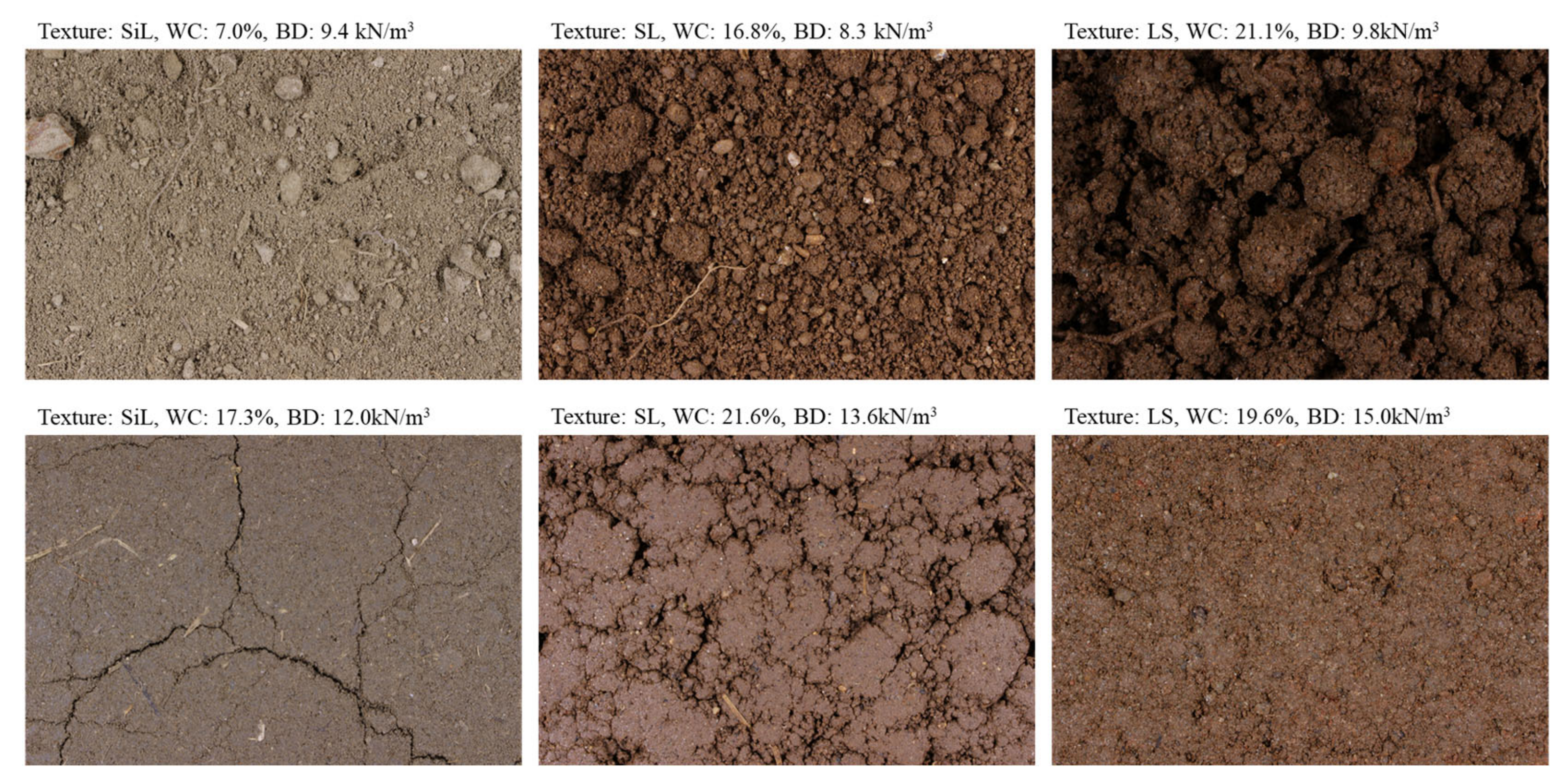
Figure 2 shows samples of soil surface images acquired at sampling points A, B, and C, along with texture, WC, and BD. Since the in situ soil surface image was taken, obstacles such as roots were also photographed on the surface layer. Depending on the texture of the soil, the color appears differently, and the color of the soil of the same texture appears differently depending on the conditions of WC and BD. At low BD, a distribution of agglomerated soil particles on the soil surface was observed. In soils with high BD, compacted soil solids were distributed on the surface and some cracks were observed. Roots that are naturally mixed with soil or cracks caused by compaction can be regarded as obstacles in soil surface images. However, as they are common elements in actual natural environments, we treated them as observation noise and included soil surface images containing them.

Table 3. Extracted features from soil surface images for deep neural network and multiple regression analysis.

	Source	Feature	Min	Mean	Max	Range
Color features	Color image	Hue	12	14.6	24.6	12.6
		Sat	37.6	108.3	168.9	131.3
		Value	57.1	126.9	183.7	126.7
	Grayscale image	Gray	41.5	105.4	172	130.5
		Skewness	−1.19	−0.27	0.82	2.01
		Kurtosis	−0.64	0.7	5.89	6.53
Texture features	Gray level co-occurrence matrix	Contrast	201.4	1185.2	2666.2	2464.8
		Dissimilarity	9.9	24.6	39.3	29.4
		Homogeneity	0.028	0.059	0.158	0.13
		Energy	0.007	0.012	0.027	0.019
		Correlation	0.1	0.47	0.8	0.7
Shape features	Hu moment	H0	0.4	0.54	0.65	0.26
		H1	1.63	1.91	2.2	0.57
		H2	3.33	4.97	8.36	5.03
		H3	3.42	5.18	7.81	4.38
		H4	−15	4.4	15.2	30.2
		H5	−10.8	3.6	8.8	19.6
		H6	−14.6	0.6	15.9	30.6

summarizes the features extracted from soil surface images in this study. A total of 18 features were extracted and used as input data for the regression model. These features were used as independent variables for multiple regression analysis and input variables for DNN regression models.

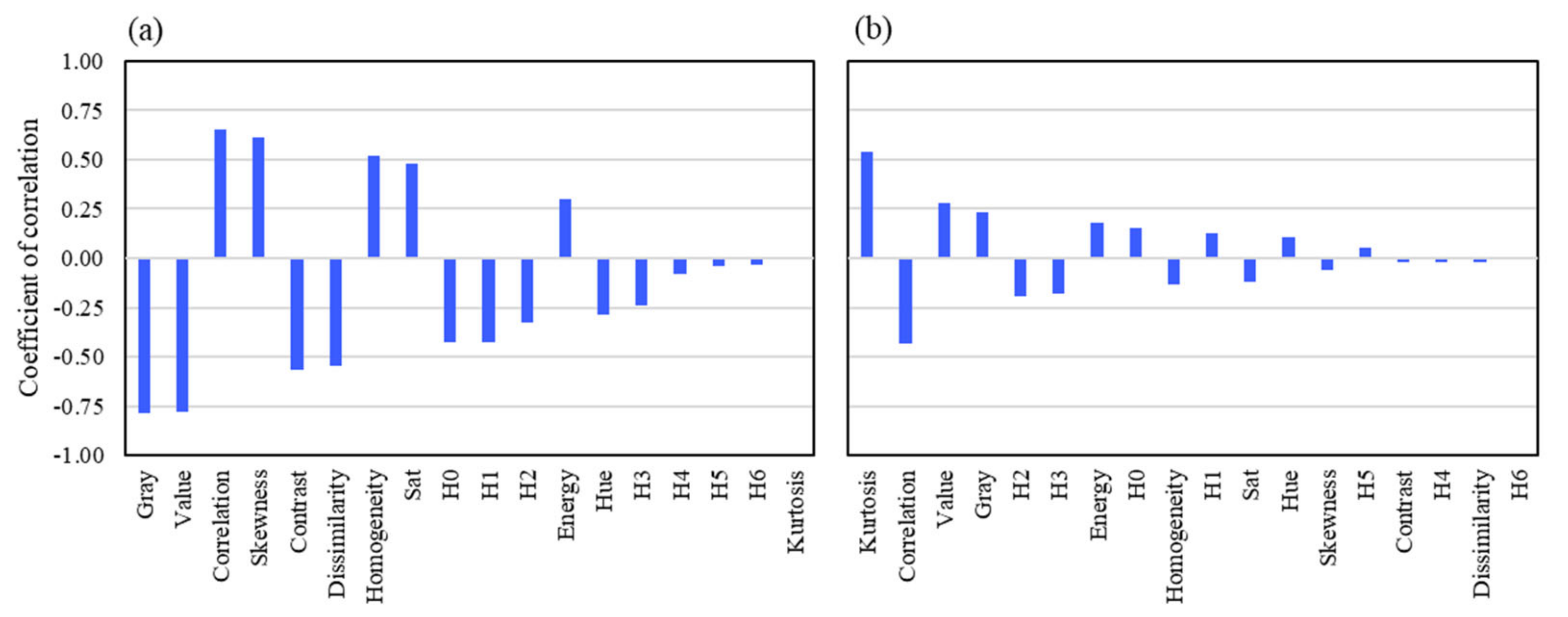
Figure 3 shows coefficient of correlation (R) between soil properties (WC, BD) and image-based features. WC and BD exhibit different correlation patterns with the various features. WC has a strong relationship ($\left|R\right|>0.75$) with Value and Gray. Additionally, WC has a moderate relationship ($0.5<\left|R\right|<0.75$) with Skewness, Contrast, Dissimilarity, Homogeneity and Correlation. BD has a moderate relationship with Kurtosis. In terms of comparing WC and BD, it can be seen that WC has a stronger relationship with image-based features than BD.

3.2. Prediction by Multiple Regression Analysis

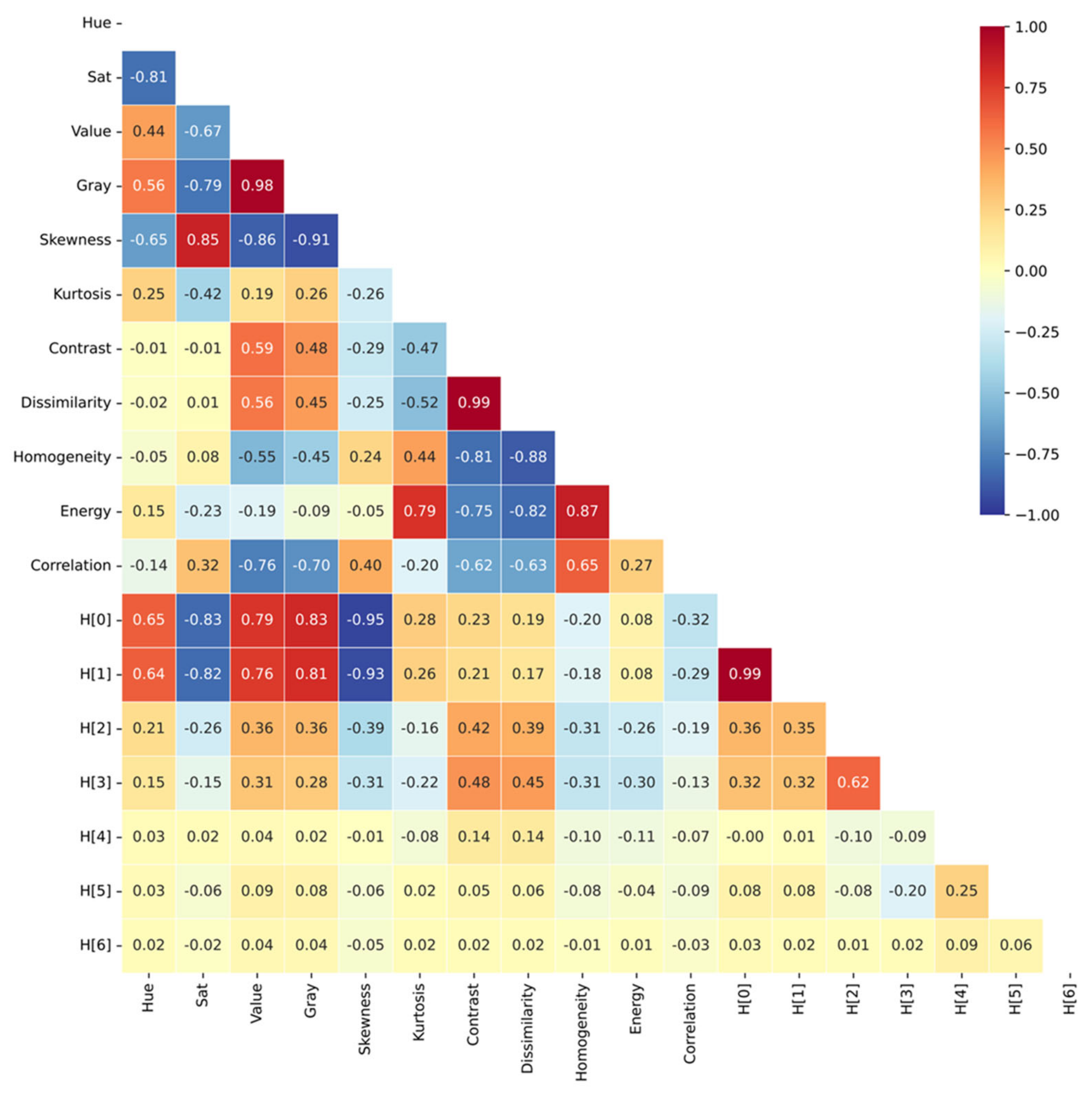
Figure 4 shows the correlation matrix of 18 soil surface image features. A number of features showed a very strong relationship, such as Value and Gray, Dissimilarity and Contrast, and H0 and H1. Hue, Sat, Value, Gray, and Skewness, which are color features, showed high correlation with H0 and H1 among shape features. Texture features showed low correlation with other features and relatively high correlation between texture features.

Table 4. Variance inflation factor of color, texture, and shape features extracted from soil surface images.

Color features	Hue	Sat	Value	Gray	Skewness	Kurtosis
VIF	194.4	529.1	8052.3	6644.8	35.2	15.9
Texture features	Contrast	Dissimilarity	Homogeneity	Energy	Correlation
VIF	875.6	3551.4	649.3	747.1	109.8
Shape features	H0	H1	H2	H3	H4	H5	H6
VIF	4926.6	7755.0	85.2	97.6	1.4	1.7	1.0

summarizes the results of calculating the VIFs of 18 soil surface image features. Since the VIF of 15 features exceeded 10, it was judged that multicollinearity would appear if these features were used in multiple regression analysis. The process of removing the feature with the highest VIF and calculating the VIF again was repeated until the VIF of all features was less than 10.

Table 5. Variance inflation factor of features for multiple regression analysis.

Features	Skewness	Kurtosis	Contrast	Correlation	H4	H5	H6
VIF	1.7	1.5	3.2	2.6	1.3	1.6	1.0

summarizes the VIF calculation results of the selected features after removing features that may affect multicollinearity. A total of seven features were selected, and all VIFs were below 10. Multiple regression analysis was performed with these as independent variables.

Table 6. Result of multiple regression analysis using features from soil surface images.

Independent Variables	Dependent Variable	Dataset	Metrics
			MAE	MAPE	R	R2	MSE	RMSE
Skewness Kurtosis Contrast Correlation H4 H5 H6	Water content (%)	A	1.39	33.1	0.96	0.92	2.92	1.71
		B	1.82	17.9	0.94	0.89	4.85	2.20
		C	1.42	9.9	0.88	0.77	3.34	1.83
		A, B, C	3.08	48.9	0.79	0.62	14.11	3.76
	Bulk density (kN/m3)	A	0.45	4.4	0.91	0.83	0.32	0.56
		B	0.54	4.9	0.91	0.83	0.47	0.68
		C	0.55	4.7	0.95	0.91	0.46	0.68
		A, B, C	1.09	9.6	0.67	0.45	1.84	1.36

summarizes the results of multiple regression analysis. For WC prediction, A showed a best performance, with an RMSE of 1.71%. B and C showed slightly lower performance than A. The model’s accuracy decreases when using the combined dataset (A, B, C). The performance of the multiple regression analysis according to the sampling point was the same in the predictions of the BD. According to the value of the MAPE, the result of the WC prediction is ‘good forecasting’ in C, and A, B and the combined dataset (A, B, C) are regarded as ‘reasonable forecasting’ [39]. The results of the BD prediction are all evaluated as ‘highly accurate forecasting’ according to MAPE [39].

3.3. Prediction by Deep Neural Network Regression Model

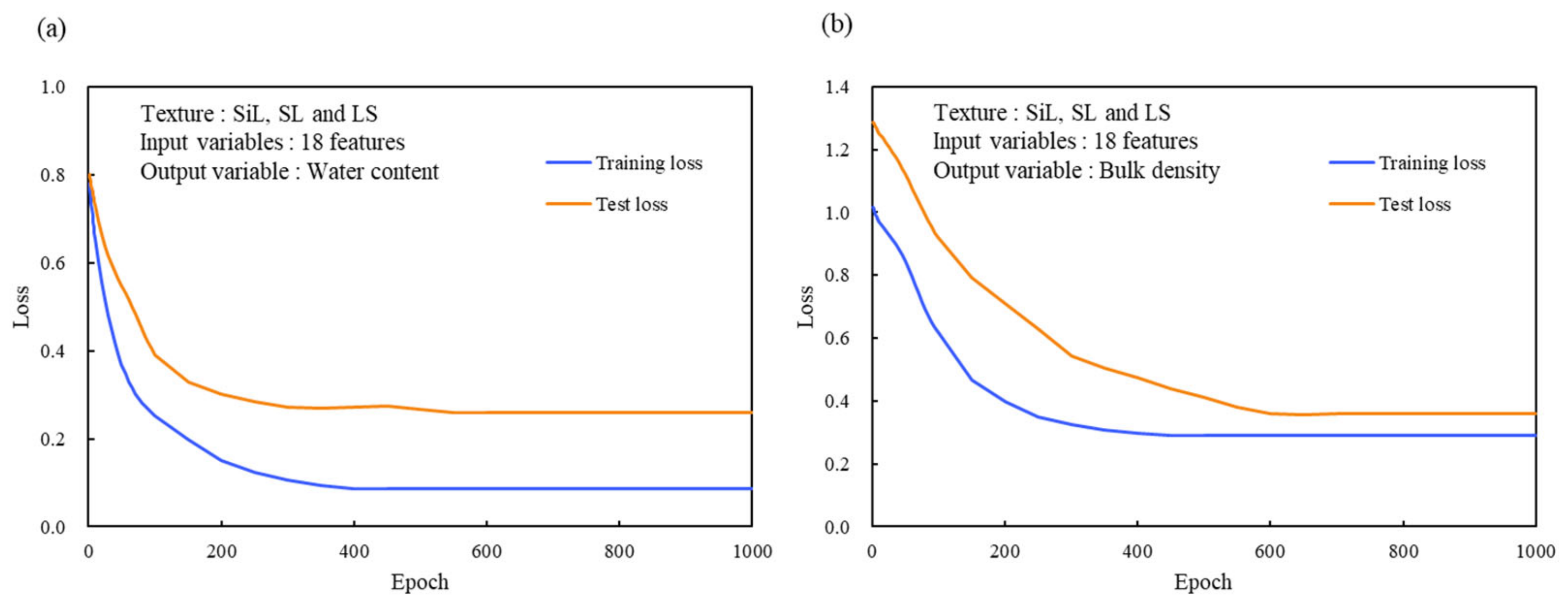
Figure 5 shows the loss curve of the DNN model. The loss is calculated using MSE, but the unit differs from the actual value due to variable normalization during the training process. Since the dataset was divided into a training set and a test set at a ratio of 8:2, and cross validation was performed by dividing the training set into five. The training loss is the average value of five validation losses. The test loss is observed to be higher than the training loss, and this shows that overfitting is not present [38].

Table 7. Result of deep neural network regression models using features from soil surface images.

Input Variables	Output Variable	Dataset	Metrics
			MAE	MAPE	R	R2	MSE	RMSE
Hue Sat Value Gray Skewness Kurtosis Contrast Dissimilarity Homogeneity Energy Correlation H0, H1, H2, H3 H4, H5, H6	Water content (%)	A	1.01	27.2	0.98	0.95	1.84	1.36
		B	1.13	11.4	0.97	0.94	2.43	1.56
		C	0.92	6.5	0.97	0.93	1.29	1.14
		A, B, C	1.23	16.9	0.97	0.94	2.32	1.52
	Bulk density (kN/m3)	A	0.36	3.6	0.95	0.91	0.20	0.45
		B	0.43	4.1	0.95	0.90	0.26	0.51
		C	0.53	4.3	0.96	0.93	0.43	0.66
		A, B, C	0.63	5.7	0.91	0.83	0.61	0.78

summarizes the performance of the DNN regression model. The results show that DNN models outperformed the multiple regression analysis models for both WC and BD prediction. Among the three sampling points, point C had the best performance for WC prediction, with an RMSE of 1.14%. For BD prediction, point A had the best performance, with an RMSE of 0.45 kN/m³. When using the combined dataset (A, B, C), the DNN models still performed better than the multiple regression analysis models, with an MAPE of 16.9% for WC prediction and 5.7% for BD prediction. However, the accuracy of the DNN models decreased slightly when using the combined dataset compared to using individual datasets, indicating that the DNN models may perform better with more specific and focused datasets. Overall, the DNN models provided more accurate prediction for both WC and BD than the multiple regression analysis models, demonstrating the potential usefulness of DNN models in soil analysis and prediction.

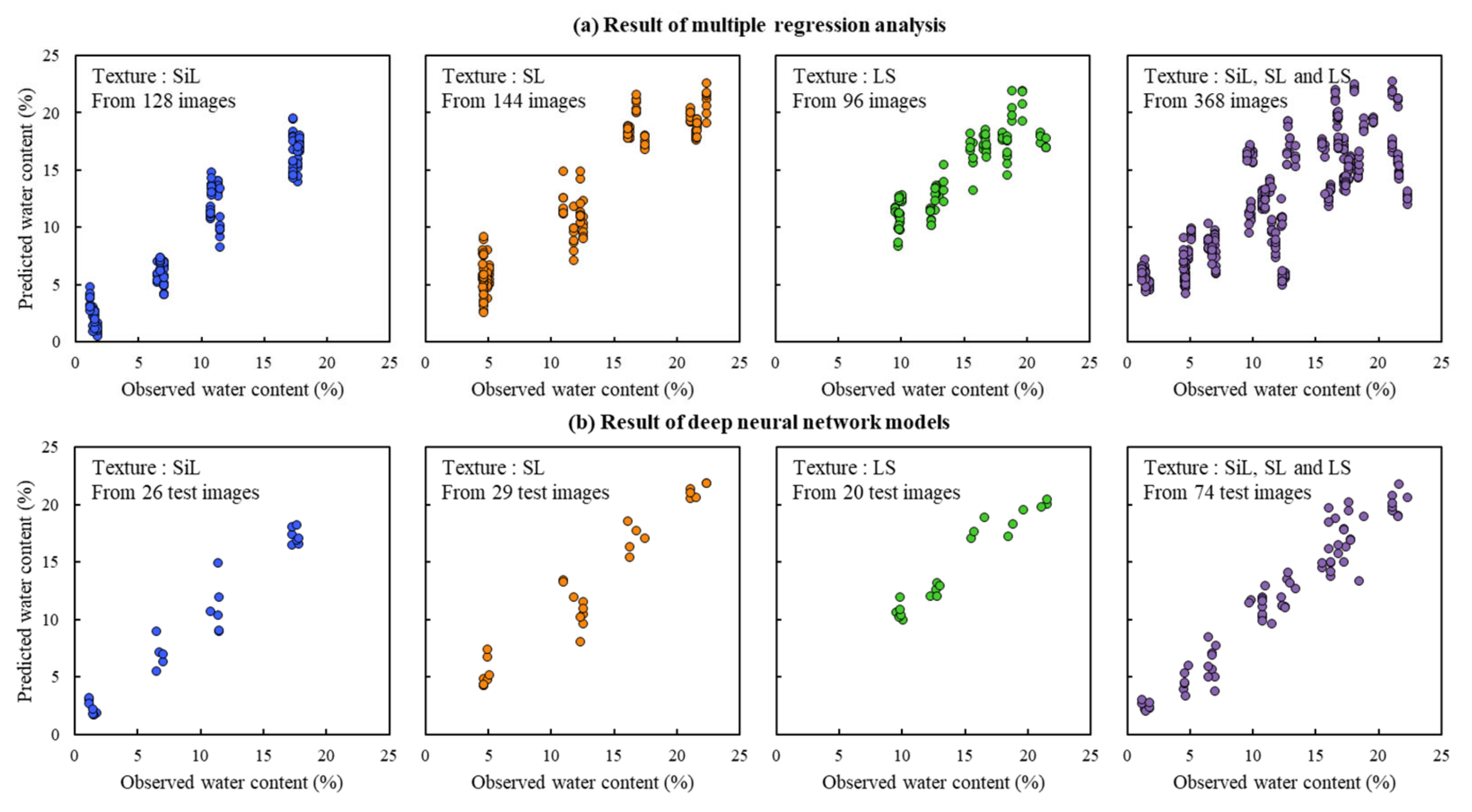
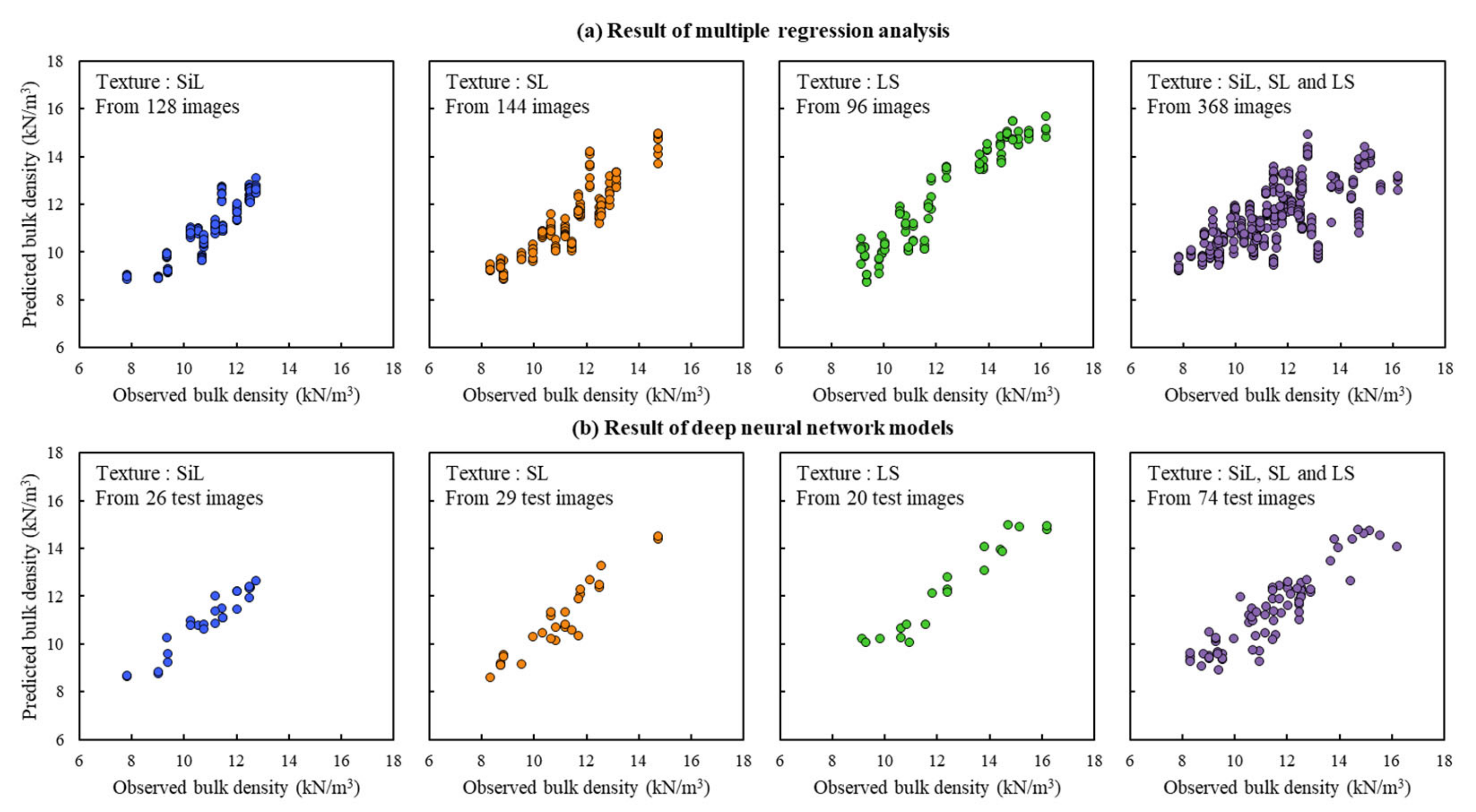
Figure 6 and Figure 7 show the scatter plot of prediction results. During training of the DNN regression model, the entire dataset was divided into a training set and a test set at a ratio of 8:2, so the data from multiple regression analysis were shown about five times larger than those from the DNN. Based on the evaluation metric, the DNN model demonstrated superior performance compared to the results obtained through multiple regression analysis. This is evident even when looking at the scatter plot of the predicted and observed values. In particular, when the entire dataset was used, the multiple regression analysis produced significantly higher variance in the prediction results, leading to lower accuracy. On the other hand, the DNN model displayed a relatively impressive performance. The reason behind this is that the DNN model has the capability to learn intricate non-linear relationships between features, enabling it to recognize differences between the features extracted from different textures of soils during the training process [38].

4. Discussion

This study aimed to predict the WC and BD through a DNN regression model, using features extracted from in situ soil surface images. The DNN regression model outperformed the multiple regression analysis, even when obstacles other than soil were present in the in situ soil surface images. This model predicted the WC and BD with high accuracy and demonstrated remarkable performance, even when learning soils of different textures together.

The significance of this study lies in its applicability in in situ agricultural land, where the prediction of surface WC and BD can help in understanding how soil affects the circulation of water resources. This is particularly important given the recent changes in climate, which necessitate the more detailed management of soil moisture in agricultural fields. Therefore, the findings of this study are expected to be highly relevant in this regard.

This study focused on soils of three textures: SiL, SL, and LS, which are widely distributed in agricultural land [40,41,42,43]. These soils have a high content of sand or silt, with a clay content of less than about 27% [1]. However, clay has a higher cohesive strength and water holding capacity than sand or silt due to their small particle size and high surface area [44]. Therefore, the color, texture, and shape features of clayey soil surface images may differ from those of the soil samples used in this study. Thus, further research is necessary to develop a more general model by adding soil textures with a high clay content.

Furthermore, the camera system used in this study has the potential to be combined with agricultural and construction machinery, enabling the easy observation of a wide area. Currently, construction equipment such as tractors, dozers, and compactors are equipped with various sensors. By combining the findings of this study with such equipment, it is anticipated that they will significantly aid in soil management at large-scale sites. Specifically, by integrating this system with a compactor at a construction site where compaction management is essential, it can play a vital role in managing the optimal moisture content and maximum dry density required for proper compaction.

Since the properties of soil can vary greatly depending on the texture, it is considered necessary to construct new training data when applying the results of this study to soils with different textures. Furthermore, as the behavior of soil may differ even among those of the same texture due to the sand, silt, and clay content, calibration becomes essential when applying the outcome of this research. If comprehensive databases on soil surface images, including those from diverse locations and textures, are secured in the future, the applicability of this study is expected to increase significantly.

In this study, the analysis was performed using color information in the visible light region, which can be obtained from digital images taken with common commercial cameras, to ensure that the study’s results can be widely applicable. The three bands of red, green, and blue were converted to HSV and grayscale color space and used to extract color, texture, and shape features. However, using multispectral or hyperspectral cameras can provide additional information beyond visible light wavelengths. If it becomes possible to acquire this information using standard image sensors in the future, we predict that more features can be extracted to enhance the model’s accuracy.

Overall, the DNN regression model, based on features extracted from in situ soil surface images, has proven to be a powerful tool for predicting WC and BD accurately. The study’s findings have great potential to impact the fields of agriculture and construction, paving the way for more effective soil management practices.

5. Conclusions

In this study, soil surface images were analyzed to predict two soil properties of WC and BD using multiple regression analysis and DNN regression models. In situ images of the soil surface were obtained and various features were extracted from them, including color, texture, and shape features. A total of 18 soil surface image features were extracted, and their relationships with soil properties were investigated. These features were used as input variables for both multiple regression analysis and DNN regression models.

The results show that WC had a stronger relationship with image-based features than BD. After removing the features that could affect multicollinearity, multiple regression analysis was performed with seven selected features as independent variables. The results showed that the multiple regression analysis models provided reasonable performance for WC and BD prediction.

Furthermore, DNN regression models were developed to predict soil properties. The results showed that the DNN models outperformed the multiple regression analysis models in terms of accuracy for both WC and BD predictions. The accuracy of the DNN models slightly decreased when using the combined dataset compared to using individual datasets. However, the DNN models still provided more accurate predictions than the multiple regression analysis models, demonstrating their potential usefulness in soil analysis and prediction.

In conclusion, this study demonstrated that soil surface images can be used to predict WC and BD, and the accuracy of the predictions can be improved by using DNN regression models. The results suggest that soil surface imaging combined with DNN models has great potential in soil analysis and prediction, which can be beneficial for precision agriculture and environmental monitoring. Further studies can be conducted to investigate the application of this method in various soil types and environments.

References

- Legrain, X.; Berding, F.; Dondeyne, S.; Schad, P.; Chapelle, J. World Reference Base for Soil Resources 2014. International Soil Classification System for Naming Soils and Creating Legends for Soil Maps; Update 2015; Food and Agriculture Organization of the United Nations: Rome, Italy, 2018. [Google Scholar]
- O’Grady, M.J.; O’Hare, G.M. Modelling the smart farm. Inf. Process. Agric. 2017, 4, 179–187. [Google Scholar] [CrossRef]
- Mulder, V.; De Bruin, S.; Schaepman, M.E.; Mayr, T. The use of remote sensing in soil and terrain mapping—A review. Geoderma 2011, 162, 1–19. [Google Scholar] [CrossRef]
- Payero, J.O.; Mirzakhani-Nafchi, A.; Khalilian, A.; Qiao, X.; Davis, R. Development of a low-cost Internet-of-Things (IoT) system for monitoring soil water potential using Watermark 200SS sensors. Adv. Internet Things 2017, 7, 71–86. [Google Scholar] [CrossRef] [Green Version]
- Klerkx, L.; Jakku, E.; Labarthe, P. A review of social science on digital agriculture, smart farming and agriculture 4.0: New contributions and a future research agenda. NJAS-Wagening J. Life Sci. 2019, 90, 100315. [Google Scholar] [CrossRef]
- Ge, Y.; Thomasson, J.A.; Sui, R. Remote sensing of soil properties in precision agriculture: A review. Front. Earth Sci. 2011, 5, 229–238. [Google Scholar] [CrossRef]
- Visconti, F.; de Paz, J.M.; Martínez, D.; Molina, M.J. Laboratory and field assessment of the capacitance sensors Decagon 10HS and 5TE for estimating the water content of irrigated soils. Agric. Water Manag. 2014, 132, 111–119. [Google Scholar] [CrossRef]
- Gunasekara Jayalath, C.P.; Gallage, C. A laboratory method for accurate calibration of strain-gauge type soil pressure transducers. In Proceedings of the 10th International Conference-Geomate 2020: Geotechnique, Construction Materials and Environment, Osaka, Japan, 16–18 November 2020; pp. 290–294. [Google Scholar]
- Amini, A.; Ramazi, H. Application of electrical resistivity imaging for engineering site investigation. A case study on prospective hospital site, Varamin, Iran. Acta Geophys. 2016, 64, 2200–2213. [Google Scholar] [CrossRef] [Green Version]
- Book, M.S.C. The Munsell Soil Colour Book; Colour Charts, Munsell Colour Company Inc.: Baltimore, MD, USA, 1992; p. 2128. [Google Scholar]
- Ritchey, E.L.; McGrath, J.M.; Gehring, D. Determining Soil Texture by Feel; Agriculture and Natural Resources Publications: Lexington, KY, USA, 2015. [Google Scholar]
- Vos, C.; Don, A.; Prietz, R.; Heidkamp, A.; Freibauer, A. Field-based soil-texture estimates could replace laboratory analysis. Geoderma 2016, 267, 215–219. [Google Scholar] [CrossRef]
- Salley, S.W.; Herrick, J.E.; Holmes, C.V.; Karl, J.W.; Levi, M.R.; McCord, S.E.; van der Waal, C.; Van Zee, J.W. A Comparison of Soil Texture-by-Feel Estimates: Implications for the Citizen Soil Scientist. Soil Sci. Soc. Am. J. 2018, 82, 1526–1537. [Google Scholar] [CrossRef]
- Morris, M.; Energy, N. Soil Moisture Monitoring: Low-Cost Tools and Methods; National Center for Appropriate Technology (NCAT): Butte, MT, USA, 2006; pp. 1–12. [Google Scholar]
- Maughan, T.; Allen, L.N.; Drost, D. Soil Moisture Measurement and Sensors for Irrigation Management; Utah State university: Logan, UT, USA, 2015. [Google Scholar]
- Aydemir, S.; Keskin, S.; Drees, L. Quantification of soil features using digital image processing (DIP) techniques. Geoderma 2004, 119, 1–8. [Google Scholar] [CrossRef]
- Bruneau, P.M.; Davidson, D.A.; Grieve, I.C. An evaluation of image analysis for measuring changes in void space and excremental features on soil thin sections in an upland grassland soil. Geoderma 2004, 120, 165–175. [Google Scholar] [CrossRef]
- O’Donnell, T.K.; Goyne, K.W.; Miles, R.J.; Baffaut, C.; Anderson, S.H.; Sudduth, K.A. Identification and quantification of soil redoximorphic features by digital image processing. Geoderma 2010, 157, 86–96. [Google Scholar] [CrossRef]
- Baek, S.-H.; Park, K.-H.; Jeon, J.-S.; Kwak, T.-Y. A Novel Method for Calibration of Digital Soil Images Captured under Irregular Lighting Conditions. Sensors 2023, 23, 296. [Google Scholar] [CrossRef] [PubMed]
- Zhao, Z.; Feng, W.; Xiao, J.; Liu, X.; Pan, S.; Liang, Z. Rapid and Accurate Prediction of Soil Texture Using an Image-Based Deep Learning Autoencoder Convolutional Neural Network Random Forest (DLAC-CNN-RF) Algorithm. Agronomy 2022, 12, 3063. [Google Scholar] [CrossRef]
- Zhang, Q.; Yang, L.T.; Chen, Z.; Li, P. A survey on deep learning for big data. Inf. Fusion 2018, 42, 146–157. [Google Scholar] [CrossRef]
- Chen, X.-W.; Lin, X. Big data deep learning: Challenges and perspectives. IEEE Access 2014, 2, 514–525. [Google Scholar] [CrossRef]
- Islam, T.; Chisty, T.A.; Chakrabarty, A. A deep neural network approach for crop selection and yield prediction in Bangladesh. In Proceedings of the 2018 IEEE Region 10 Humanitarian Technology Conference (R10-HTC), Malambe, Sri Lanka, 6–8 December 2018; pp. 1–6. [Google Scholar]
- Kumar, S.; Sharma, B.; Sharma, V.K.; Poonia, R.C. Automated soil prediction using bag-of-features and chaotic spider monkey optimization algorithm. Evol. Intell. 2021, 14, 293–304. [Google Scholar] [CrossRef]
- Wu, J.; Yin, X.; Xiao, H. Seeing permeability from images: Fast prediction with convolutional neural networks. Sci. Bull. 2018, 63, 1215–1222. [Google Scholar] [CrossRef] [Green Version]
- Mouazen, A.; Karoui, R.; Deckers, J.; De Baerdemaeker, J.; Ramon, H. Potential of visible and near-infrared spectroscopy to derive colour groups utilising the Munsell soil colour charts. Biosyst. Eng. 2007, 97, 131–143. [Google Scholar] [CrossRef]
- Haralick, R.M.; Shanmugam, K.; Dinstein, I.H. Textural features for image classification. IEEE Trans. Syst. Man Cybern. 1973, SMC-3, 610–621. [Google Scholar] [CrossRef] [Green Version]
- Hu, M.-K. Visual pattern recognition by moment invariants. IRE Trans. Inf. Theory 1962, 8, 179–187. [Google Scholar]
- Craney, T.A.; Surles, J.G. Model-dependent variance inflation factor cutoff values. Qual. Eng. 2002, 14, 391–403. [Google Scholar] [CrossRef]
- Miles, J. Tolerance and variance inflation factor. In Wiley Statsref: Statistics Reference Online; Wiley: New York, NY, USA, 2014. [Google Scholar]
- Rodriguez, J.D.; Perez, A.; Lozano, J.A. Sensitivity analysis of k-fold cross validation in prediction error estimation. IEEE Trans. Pattern Anal. Mach. Intell. 2009, 32, 569–575. [Google Scholar] [CrossRef]
- Wong, T.-T.; Yeh, P.-Y. Reliable Accuracy Estimates from k-Fold Cross Validation. IEEE Trans. Knowl. Data Eng. 2020, 32, 1586–1594. [Google Scholar] [CrossRef]
- Bergstra, J.; Bengio, Y. Random search for hyper-parameter optimization. J. Mach. Learn. Res. 2012, 13, 281–305. [Google Scholar]
- Smith, L.N. A disciplined approach to neural network hyper-parameters: Part 1--learning rate, batch size, momentum, and weight decay. arXiv 2018, arXiv:1803.09820. [Google Scholar]
- Xiao, X.; Yan, M.; Basodi, S.; Ji, C.; Pan, Y. Efficient hyperparameter optimization in deep learning using a variable length genetic algorithm. arXiv 2020, arXiv:2006.12703. [Google Scholar]
- Bengio, Y.; Courville, A.; Vincent, P. Representation learning: A review and new perspectives. IEEE Trans. Pattern Anal. Mach. Intell. 2013, 35, 1798–1828. [Google Scholar] [CrossRef] [Green Version]
- Géron, A. Hands-on Machine Learning with Scikit-Learn and Tensorflow: Concepts; Tools, and Techniques to Build Intelligent Systems; O’Reilly Media, Inc.: Newton, MA, USA, 2017. [Google Scholar]
- Goodfellow, I.; Bengio, Y.; Courville, A. Deep Learning; MIT Press: Cambridge, MA, USA, 2016. [Google Scholar]
- Lewis, C.D. Industrial and Business Forecasting Methods: A Practical Guide to Exponential Smoothing and Curve Fitting; Butterworth-Heinemann: Woburn, MA, USA, 1982. [Google Scholar]
- Han, K.-H.; Zhang, Y.-S.; Jung, K.-H.; Cho, H.-R.; Seo, M.-J.; Sonn, Y.-K. Statistically estimated storage potential of organic carbon by its association with clay content for Korean upland subsoil. Korean J. Agric. Sci. 2016, 43, 353–359. [Google Scholar] [CrossRef] [Green Version]
- Pásztor, L.; Négyesi, G.; Laborczi, A.; Kovács, T.; László, E.; Bihari, Z. Integrated spatial assessment of wind erosion risk in Hungary. Nat. Hazards Earth Syst. Sci. 2016, 16, 2421–2432. [Google Scholar] [CrossRef] [Green Version]
- Rodrigues, L.; Lombardo, U.; Trauerstein, M.; Huber, P.; Mohr, S.; Veit, H. An insight into pre-Columbian raised fields: The case of San Borja, Bolivian lowlands. Soil 2016, 2, 367–389. [Google Scholar] [CrossRef] [Green Version]
- Ok, J.-h.; Kim, D.-J.; Han, K.-h.; Jung, K.-H.; Lee, K.-D.; Zhang, Y.-s.; Cho, H.-r.; Hwang, S.-a. Relationship between measured and predicted soil water content using soil moisture monitoring network. Korean J. Agric. For. Meteorol. 2019, 21, 297–306. [Google Scholar]
- Brady, N.C.; Weil, R.R.; Weil, R.R. The Nature and Properties of Soils; Prentice Hall: Upper Saddle River, NJ, USA, 2008; Volume 13. [Google Scholar]