
Performance Assessment of Bias Correction Methods for Precipitation and Temperature from CMIP5 Model Simulation


Abstract
:1. Introduction
2. Study Area and Datasets Used
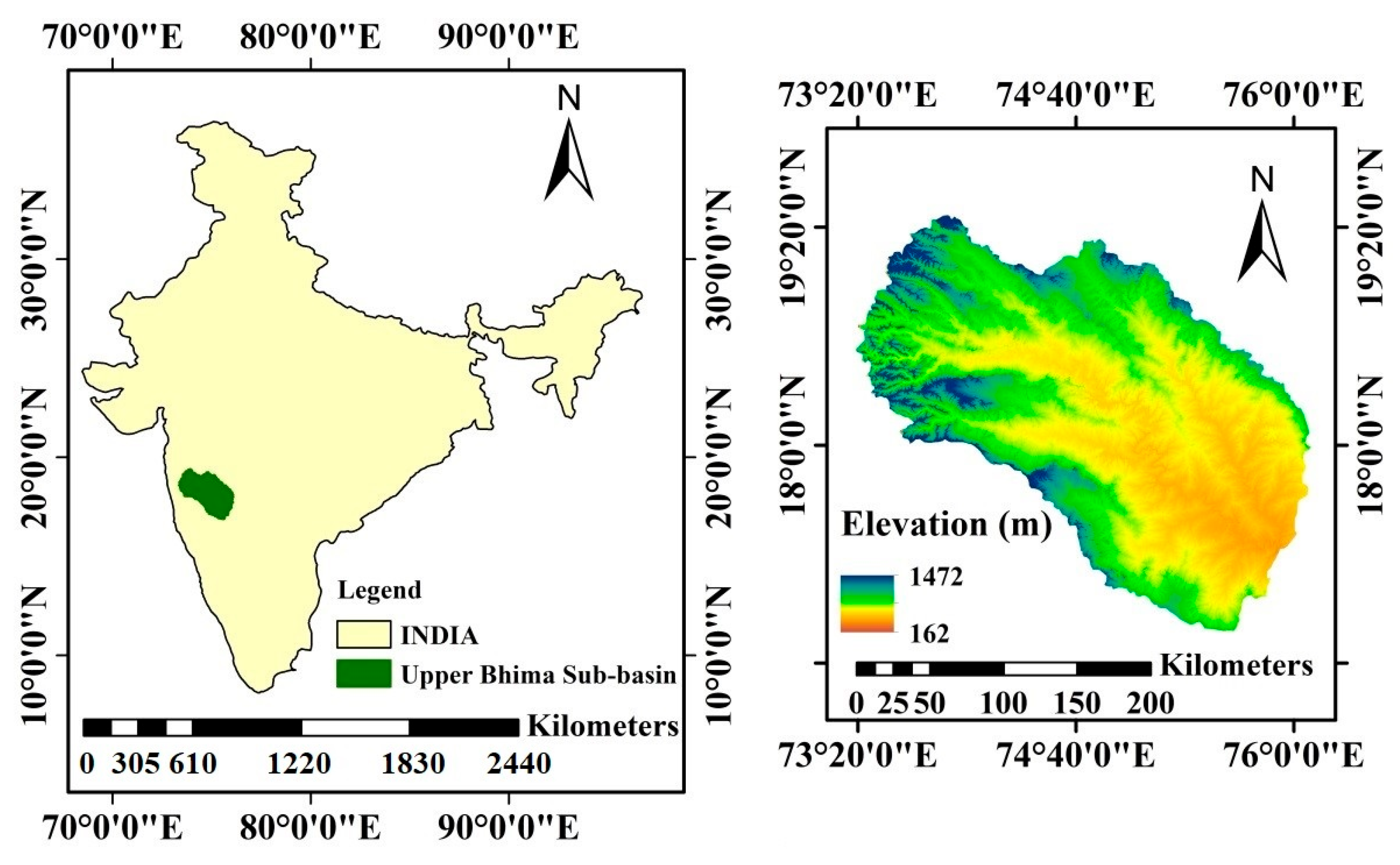
2.1. Study Area
2.2. Datasets
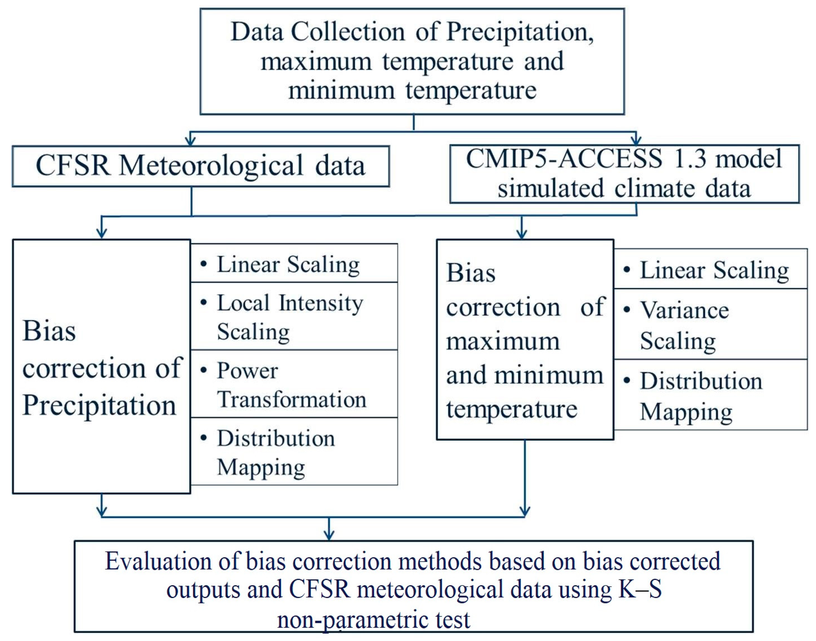
3. Methodology
3.1. Bias Correction Methods
3.1.1. Linear Scaling (LS) of Precipitation and Temperature
3.1.2. Local Intensity Scaling (LOCI) of Precipitation
3.1.3. Power Transformation (PT) of Precipitation
3.1.4. Variance Scaling (VARI) of Temperature
3.1.5. Distribution Mapping (DM) of Precipitation and Temperature
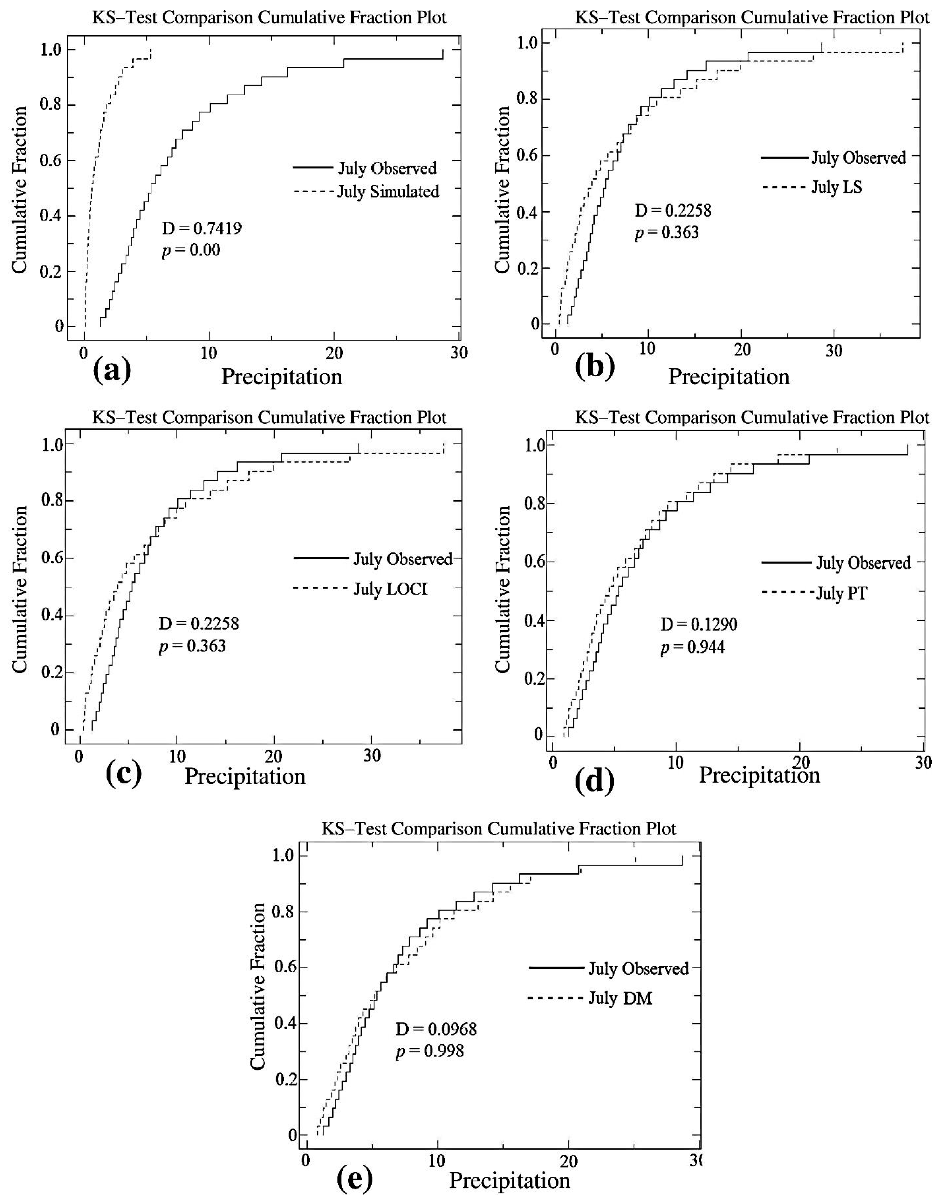
3.2. Kolmogorov–Smirnov Non-Parametric Test
4. Results and Discussion
4.1. Evaluation of CMIP5 Global Climate Models Used in the Analysis
4.1.1. Precipitation
4.1.2. Maximum and Minimum Temperature
Maximum Temperature

| Models | MBE | MAE | RMSE | NSE | Correlation Coefficient |
|---|---|---|---|---|---|
| ACCESS1.3 | 0.959 | 2.358 | 7.806 | 0.224 | 0.486 |
| CMCC-CESM | 1.092 | 2.498 | 7.783 | 0.229 | 0.494 |
| CNRM-CM5 | 1.018 | 2.428 | 7.768 | 0.232 | 0.495 |
| GFDL-CM3 | 0.984 | 2.353 | 7.759 | 0.234 | 0.496 |
| HadCM3 | 1.013 | 2.982 | 7.941 | 0.197 | 0.466 |
| HADGEM2-ES | 1.005 | 2.976 | 8.022 | 0.181 | 0.45 |
| INM-CM4 | 0.993 | 2.308 | 7.659 | 0.253 | 0.515 |
| MIROC5 | 0.926 | 2.425 | 7.772 | 0.231 | 0.492 |
| MPI-ESM-P | 1.029 | 2.277 | 7.715 | 0.242 | 0.506 |
| MRI-CGCM3 | 1.034 | 2.64 | 7.855 | 0.215 | 0.479 |
| MRI-ESM1 | 0.978 | 2.506 | 7.791 | 0.227 | 0.49 |
| NorESM1_M | 0.968 | 2.485 | 7.834 | 0.219 | 0.481 |
Minimum Temperature
| Models | MBE | MAE | RMSE | NSE | Correlation Coefficient |
|---|---|---|---|---|---|
| ACCESS1.3 | 0.87 | 1.693 | 6.862 | 0.208 | 0.472 |
| CMCC-CESM | 0.914 | 1.924 | 6.914 | 0.196 | 0.459 |
| CNRM-CM5 | 0.846 | 1.762 | 6.895 | 0.201 | 0.462 |
| GFDL-CM3 | 0.89 | 1.792 | 6.93 | 0.193 | 0.454 |
| HadCM3 | 0.905 | 2.181 | 7.005 | 0.175 | 0.435 |
| HADGEM2-ES | 0.893 | 2.135 | 7.074 | 0.159 | 0.417 |
| INM-CM4 | 0.893 | 1.757 | 6.9 | 0.2 | 0.462 |
| MIROC5 | 0.773 | 1.895 | 6.908 | 0.198 | 0.456 |
| MPI-ESM-P | 0.847 | 1.818 | 6.819 | 0.218 | 0.482 |
| MRI-CGCM3 | 0.907 | 1.83 | 6.771 | 0.229 | 0.497 |
| MRI-ESM1 | 0.862 | 1.854 | 6.944 | 0.189 | 0.449 |
| NorESM1_M | 0.793 | 1.958 | 6.956 | 0.186 | 0.444 |
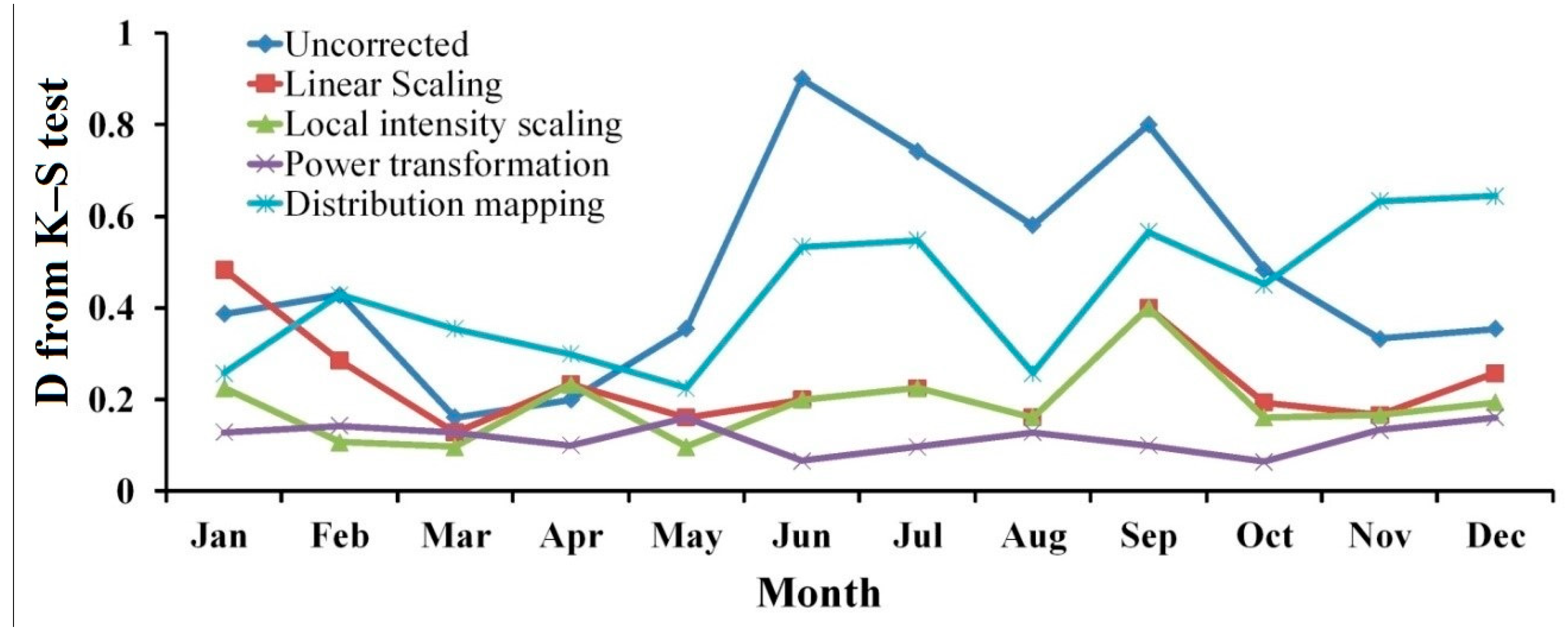
4.2. Statistical Analysis of Kolmogorov–Smirnov Test
4.2.1. Precipitation
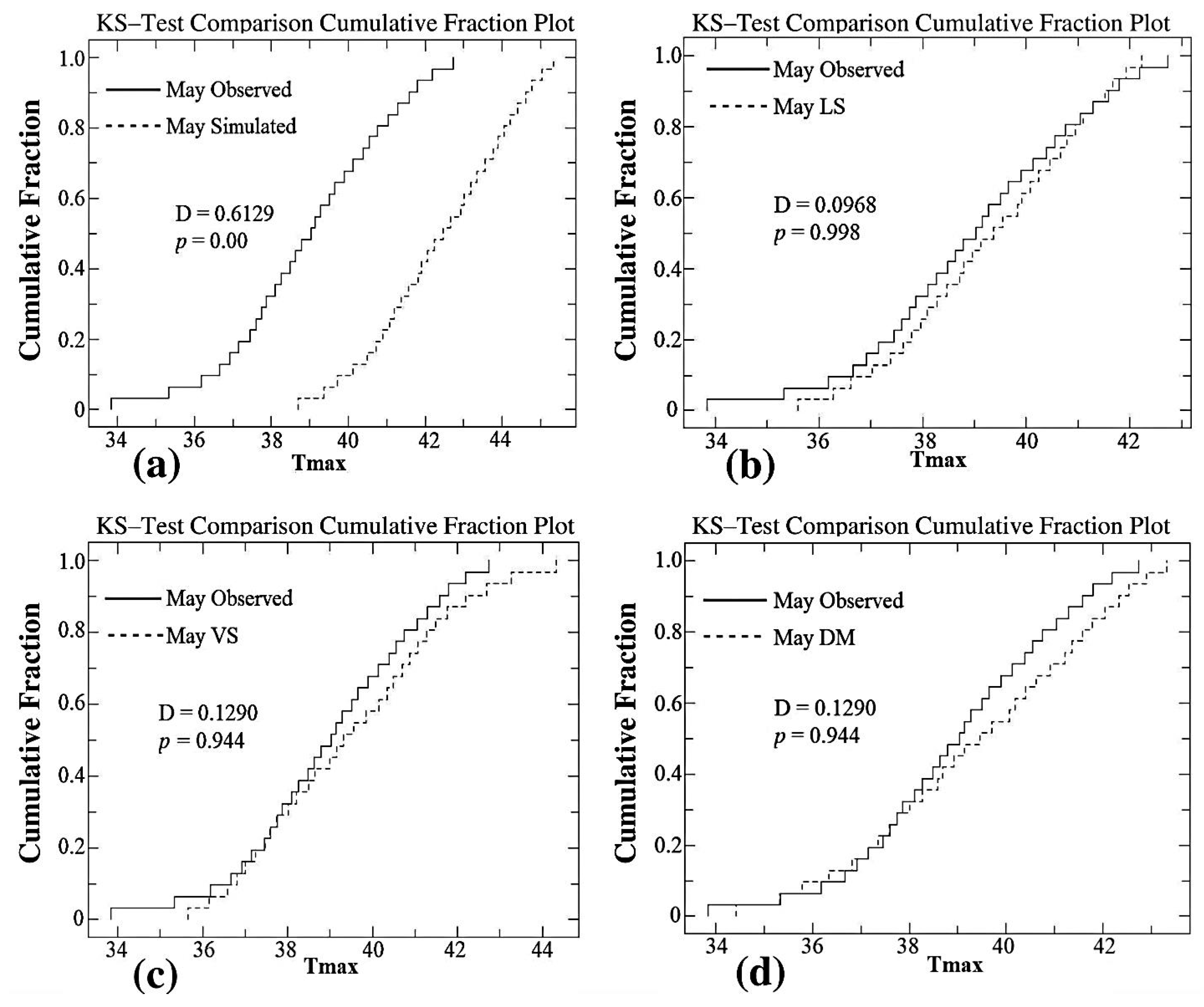
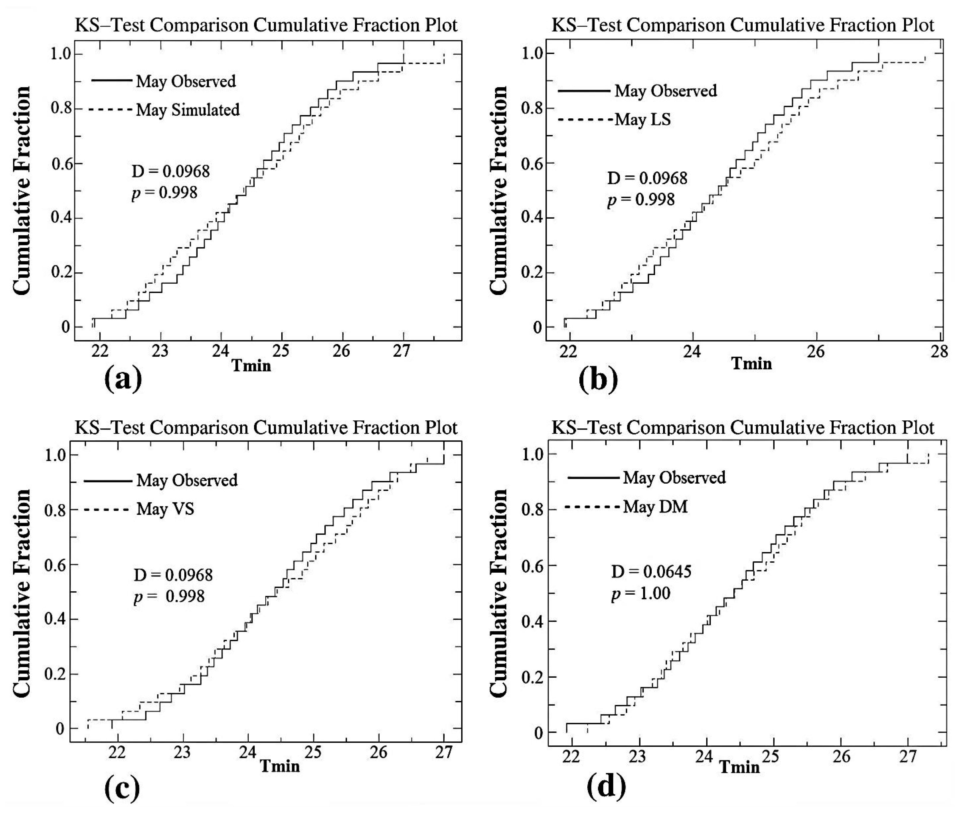
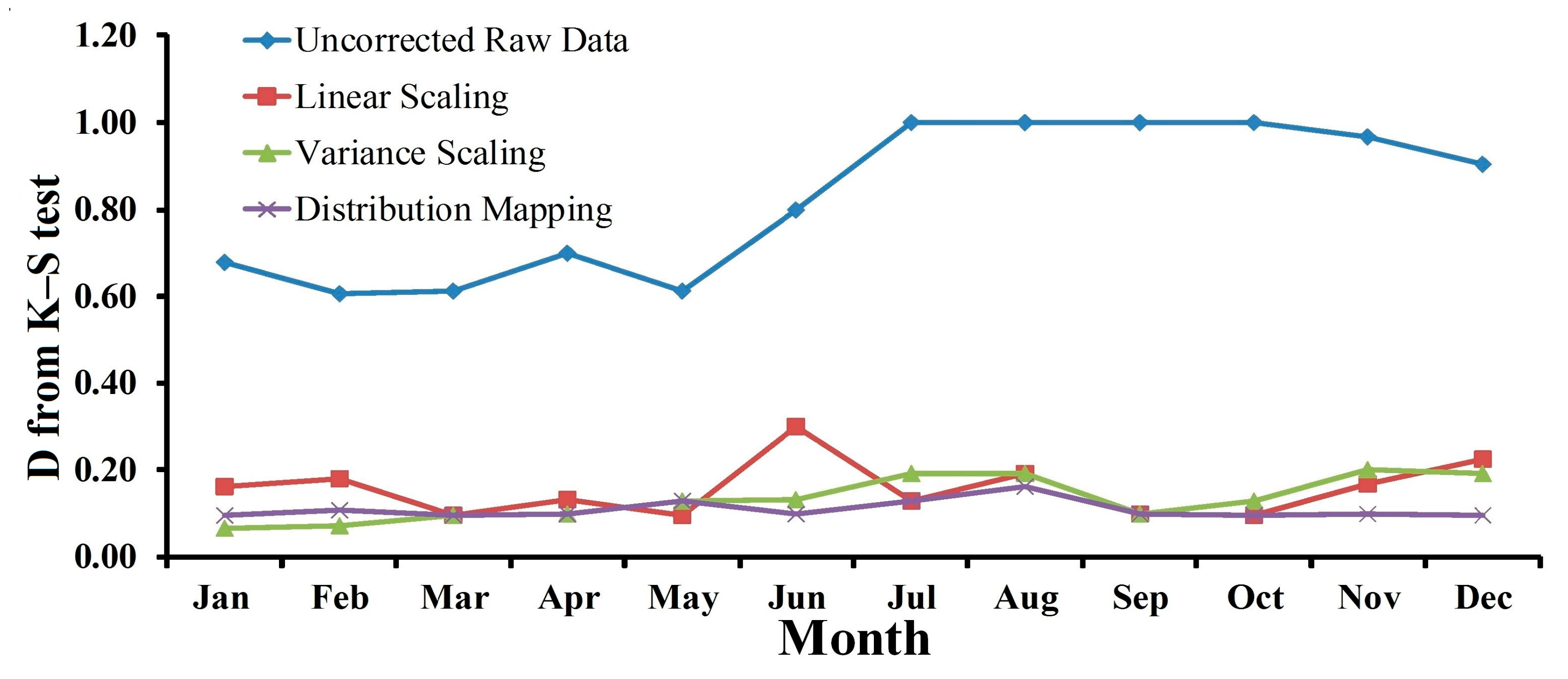
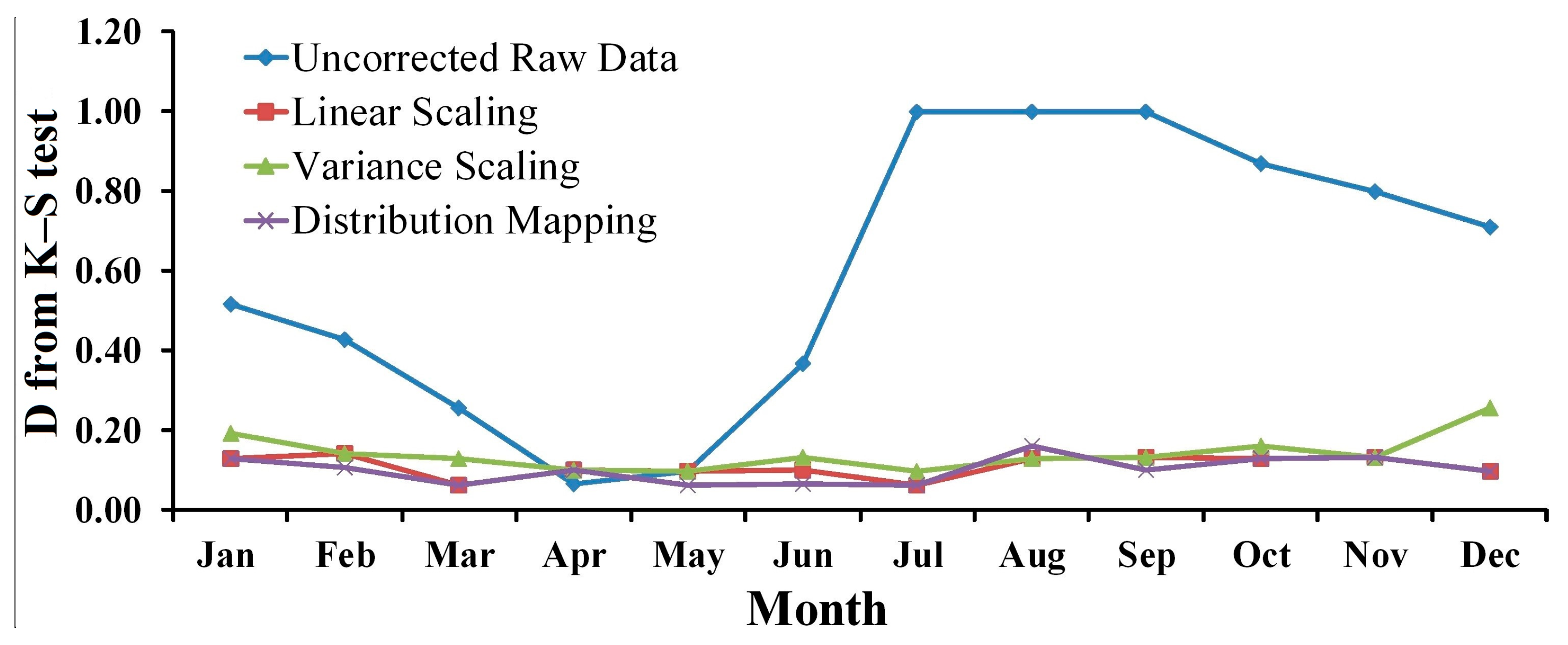
4.2.2. Maximum and Minimum Temperature (Tmax and Tmin)
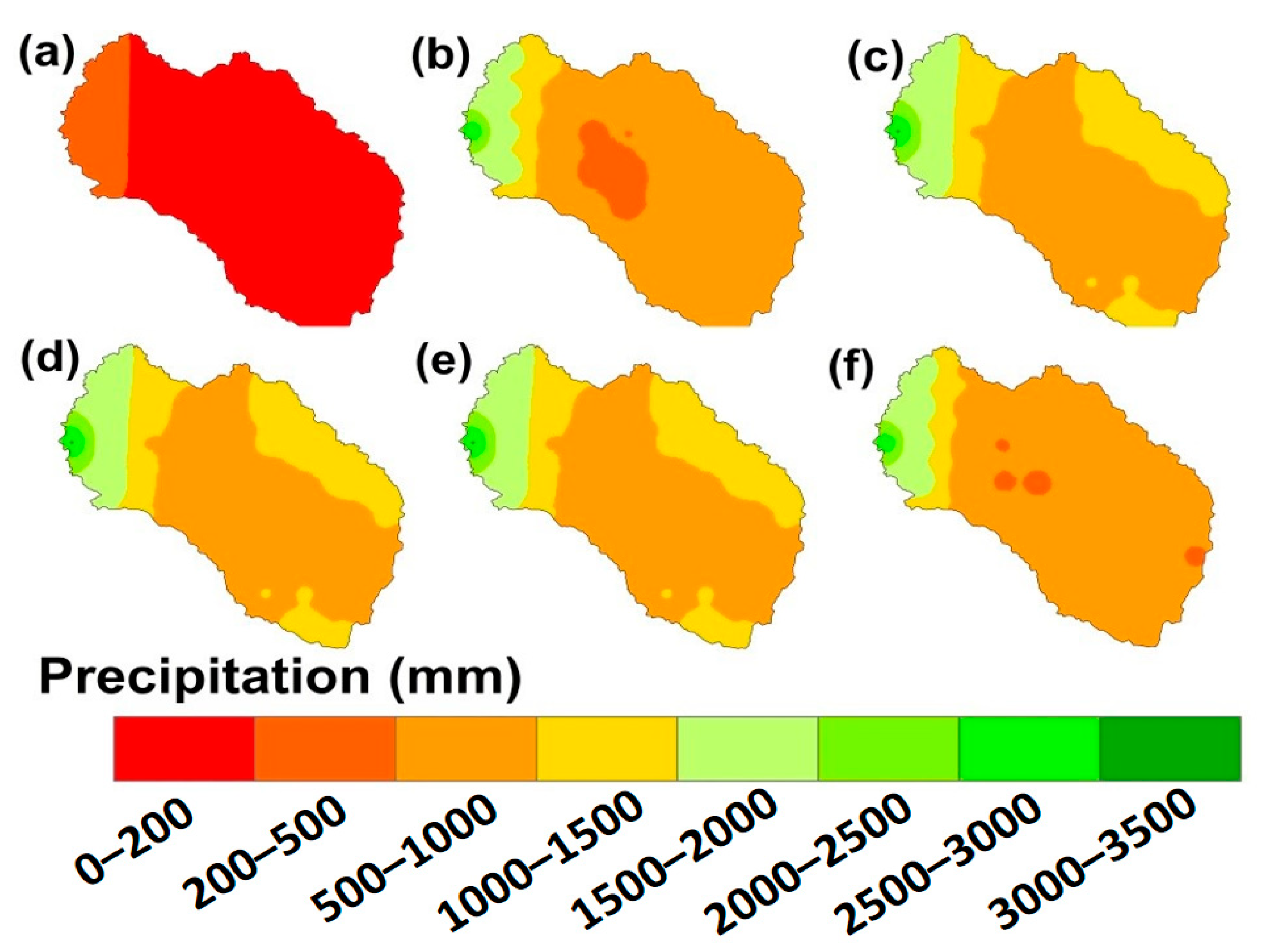
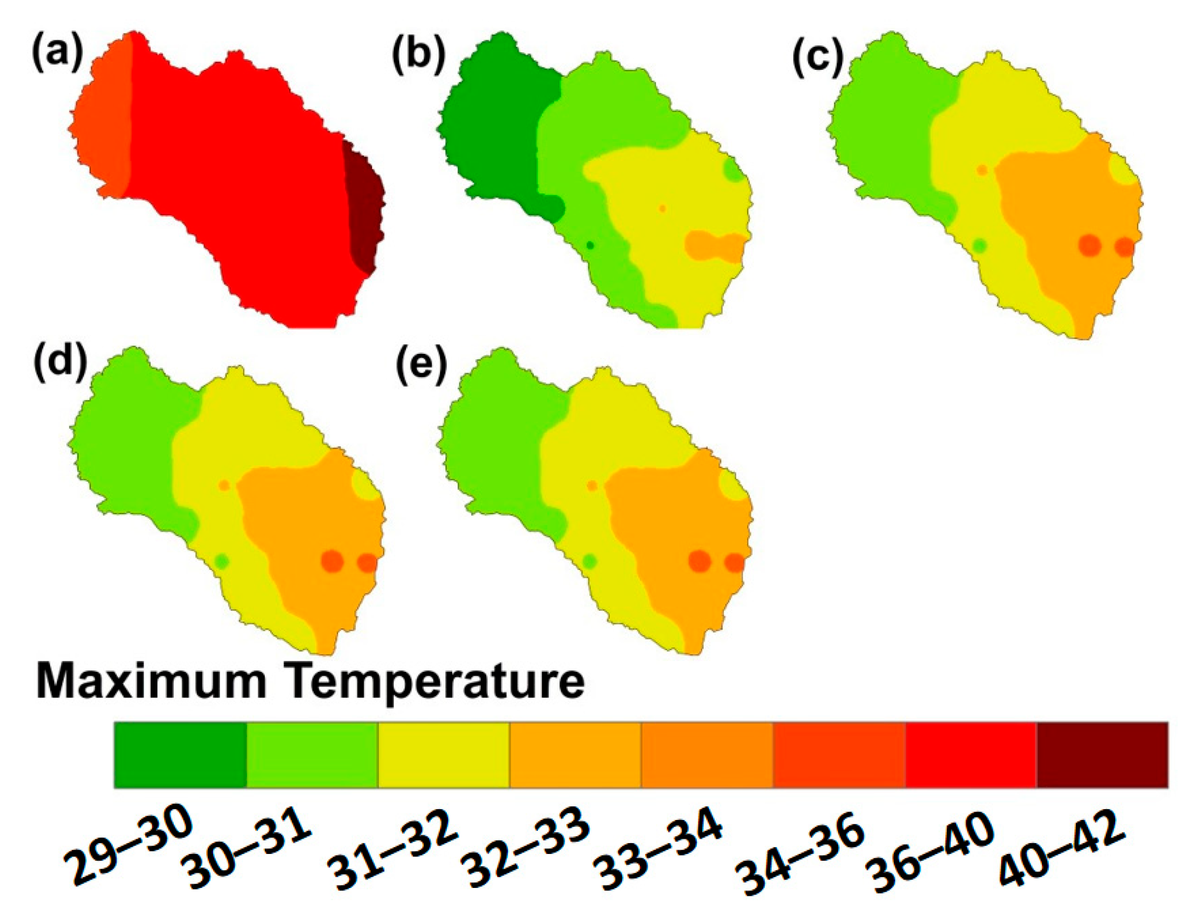
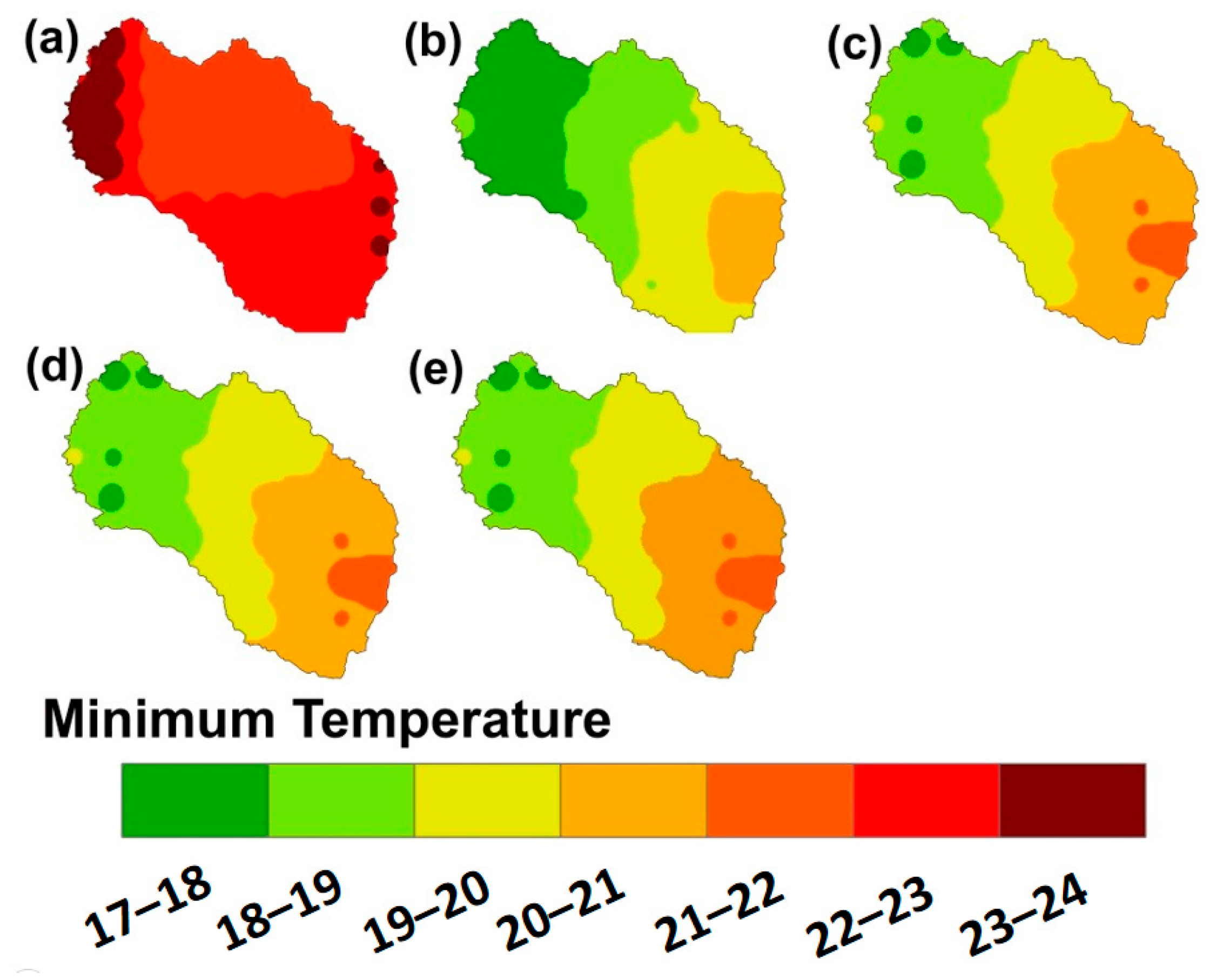
4.3. Spatial Variation of Precipitation, Maximum Temperature, and Minimum Temperature
4.3.1. Precipitation
4.3.2. Maximum Temperature
4.3.3. Minimum Temperature
5. Conclusions
Supplementary Materials
Author Contributions
Funding
Institutional Review Board Statement
Informed Consent Statement
Data Availability Statement
Conflicts of Interest
References
- Revadekar, J.V.; Preethi, B. Statistical analysis of the relationship between summer monsoon precipitation extremes and foodgrain yield over India. Int. J. Climatol. 2012, 32, 419–429. [Google Scholar] [CrossRef]
- Mpelasoka, F.S.; Chiew, F.H. Influence of rainfall scenario construction methods on runoff projections. J. Hydrometeorol. 2009, 10, 1168–1183. [Google Scholar] [CrossRef]
- Kumar, K.R.; Sahai, A.K.; Kumar, K.K.; Patwardhan, S.K.; Mishra, P.K.; Revadekar, J.V.; Kamala, K.; Pant, G.B. High-resolution climate change scenarios for India for the 21st century. Curr. Sci. 2006, 90, 334–345. [Google Scholar]
- Teutschbein, C.; Seibert, J. Regional climate models for hydrological impact studies at the catchment scale: A review of recent modeling strategies. Geogr. Compass 2010, 4, 834–860. [Google Scholar]
- Luo, M.; Liu, T.; Meng, F.; Duan, Y.; Frankl, A.; Bao, A.; De Maeyer, P. Comparing bias correction methods used in downscaling precipitation and temperature from regional climate models: A case study from the Kaidu River Basin in Western China. Water 2018, 10, 1046. [Google Scholar]
- Liu, C.; Allan, R.P. Observed and simulated precipitation responses in wet and dry regions 1850–2100. Environ. Res. Lett. 2013, 8, 034002. [Google Scholar] [CrossRef]
- Chadwick, R.; Good, P.; Martin, G.; Rowell, D.P. Large rainfall changes consistently projected over substantial areas of tropical land. Nat. Clim. Change 2016, 6, 177–181. [Google Scholar] [CrossRef]
- Daksiya, V.; Mandapaka, P.; Lo, E.Y. A comparative frequency analysis of maximum daily rainfall for a SE Asian region under current and future climate conditions. Adv. Meteorol. 2017, 2017, 1–16. [Google Scholar] [CrossRef] [Green Version]
- Valappil, V.K.; Temimi, M.; Weston, M.; Fonseca, R.; Nelli, N.R.; Thota, M.; Kumar, K.N. Assessing Bias correction methods in support of operational weather forecast in arid environment. Asia-Pac. J. Atmos. Sci. 2020, 56, 333–347. [Google Scholar] [CrossRef]
- Shin, S.W.; Kim, T.J.; Kim, J.U.; Goo, T.Y.; Byun, Y.H. Application of bias-and variance-corrected SST on wintertime precipitation simulation of regional climate model over East Asian Region. Asia-Pac. J. Atmos. Sci. 2021, 57, 387–404. [Google Scholar] [CrossRef]
- Teutschbein, C.; Seibert, J. Bias correction of regional climate model simulations for hydrological climate-change impact studies: Review and evaluation of different methods. J. Hydrol. 2012, 456, 12–29. [Google Scholar] [CrossRef]
- Ghimire, U.; Srinivasan, G.; Agarwal, A. Assessment of rainfall bias correction techniques for improved hydrological simulation. Int. J. Climatol. 2019, 39, 2386–2399. [Google Scholar] [CrossRef]
- Wood, A.W.; Leung, L.R.; Sridhar, V.; Lettenmaier, D.P. Hydrologic implications of dynamical and statistical approaches to downscaling climate model outputs. Clim. Change 2004, 62, 189–216. [Google Scholar] [CrossRef]
- Parry, M.L.; Canziani, O.; Palutikof, J.; Van der Linden, P.; Hanson, C. (Eds.) Climate Change 2007—Impacts, Adaptation and Vulnerability: Working Group II Contribution to the Fourth Assessment Report of the IPCC; Cambridge University Press: Cambridge, UK, 2007; Volume 4. [Google Scholar]
- Hawkins, E.; Osborne, T.M.; Ho, C.K.; Challinor, A.J. Calibration and bias correction of climate projections for crop modelling: An idealised case study over Europe. Agric. For. Meteorol. 2013, 170, 19–31. [Google Scholar] [CrossRef]
- Seaby, L.P.; Refsgaard, J.C.; Sonnenborg, T.O.; Højberg, A.L. Spatial uncertainty in bias corrected climate change projections and hydrogeological impacts. Hydrol. Process. 2015, 29, 4514–4532. [Google Scholar] [CrossRef]
- Iizumi, T.; Takikawa, H.; Hirabayashi, Y.; Hanasaki, N.; Nishimori, M. Contributions of different bias-correction methods and reference meteorological forcing data sets to uncertainty in projected temperature and precipitation extremes. J. Geophys. Res. Atmos. 2017, 122, 7800–7819. [Google Scholar] [CrossRef] [Green Version]
- Zollo, A.L.; Rianna, G.; Mercogliano, P.; Tommasi, P.; Comegna, L. Validation of a simulation chain to assess climate change impact on precipitation induced landslides. In Landslide Science for a Safer Geoenvironment: Vol. 1: The International Programme on Landslides (IPL); Springer International Publishing: New York, NY, USA, 2014; pp. 287–292. [Google Scholar]
- Crochemore, L.; Ramos, M.H.; Pappenberger, F. Bias correcting precipitation forecasts to improve the skill of seasonal streamflow forecasts. Hydrol. Earth Syst. Sci. 2016, 20, 3601–3618. [Google Scholar] [CrossRef] [Green Version]
- Schmidli, J.; Frei, C.; Vidale, P.L. Downscaling from GCM precipitation: A benchmark for dynamical and statistical downscaling methods. Int. J. Climatol. J. R. Meteorol. Soc. 2006, 26, 679–689. [Google Scholar] [CrossRef]
- Lenderink, G.; Buishand, A.; Van Deursen, W. Estimates of future discharges of the river Rhine using two scenario methodologies: Direct versus delta approach. Hydrol. Earth Syst. Sci. 2007, 11, 1145–1159. [Google Scholar] [CrossRef]
- Chen, J.; Brissette, F.P.; Chaumont, D.; Braun, M. Performance and uncertainty evaluation of empirical downscaling methods in quantifying the climate change impacts on hydrology over two North American river basins. J. Hydrol. 2013, 479, 200–214. [Google Scholar] [CrossRef]
- White, R.H.; Toumi, R. The limitations of bias correcting regional climate model inputs. Geophys. Res. Lett. 2013, 40, 2907–2912. [Google Scholar] [CrossRef]
- Pavelic, P.; Patankar, U.; Acharya, S.; Jella, K.; Gumma, M.K. Role of groundwater in buffering irrigation production against climate variability at the basin scale in South-West India. Agric. Water Manag. 2012, 103, 78–87. [Google Scholar] [CrossRef]
- Trenberth, K.E.; Jones, P.D.; Ambenje, P.; Bojariu, R.; Easterling, D.; Klein Tank, A.; Rusticucci, M. Climate change 2007: The physical science basis. Clim. Change 2007, 6, 235–336. [Google Scholar]
- Fuka, D.R.; Walter, M.T.; MacAlister, C.; Degaetano, A.T.; Steenhuis, T.S.; Easton, Z.M. Using the Climate Forecast System Reanalysis as weather input data for watershed models. Hydrol. Process. 2014, 28, 5613–5623. [Google Scholar] [CrossRef]
- Piani, C.; Weedon, G.P.; Best, M.; Gomes, S.M.; Viterbo, P.; Hagemann, S.; Haerter, J.O. Statistical bias correction of global simulated daily precipitation and temperature for the application of hydrological models. J. Hydrol. 2010, 395, 199–215. [Google Scholar] [CrossRef]
- Piani, C.; Haerter, J.O.; Coppola, E. Statistical bias correction for daily precipitation in regional climate models over Europe. Theor. Appl. Climatol. 2010, 99, 187–192. [Google Scholar] [CrossRef] [Green Version]
- Maraun, D.; Wetterhall, F.; Ireson, A.M.; Chandler, R.E.; Kendon, E.J.; Widmann, M.; Brienen, S.; Rust, H.W.; Sauter, T.; Themeßl, M.; et al. Precipitation downscaling under climate change: Recent developments to bridge the gap between dynamical models and the end user. Rev. Geophys. 2010, 48. [Google Scholar] [CrossRef] [Green Version]
- Terink, W.; Hurkmans, R.T.W.L.; Torfs, P.J.J.F.; Uijlenhoet, R. Evaluation of a bias correction method applied to downscaled precipitation and temperature reanalysis data for the Rhine basin. Hydrol. Earth Syst. Sci. 2010, 14, 687–703. [Google Scholar] [CrossRef] [Green Version]
- Themeßl, M.J.; Gobiet, A.; Heinrich, G. Empirical-statistical downscaling and error correction of regional climate models and its impact on the climate change signal. Clim. Change 2012, 112, 449–468. [Google Scholar] [CrossRef]
- Thom, H.C. A note on the gamma distribution. Mon. Weather Rev. 1958, 86, 117–122. [Google Scholar] [CrossRef]
- Kim, P.J. On the exact and approximate sampling distribution of the two sample Kolmogorov-Smirnov criterion dmn, m ≤ n. J. Am. Stat. Assoc. 1969, 64, 1625–1637. [Google Scholar] [CrossRef]
- Press, W.H.; Teukolsky, S.A.; Vetterling, W.T.; Flannery, B.P. Numerical recipes in C; Cambridge University: Cambridge, UK, 1992. [Google Scholar]
- Rishma, C.; Katpatal, Y.B. ENSO modulated groundwater variations in a river basin of Central India. Hydrol. Res. 2019, 50, 793–806. [Google Scholar] [CrossRef] [Green Version]
- Tschöke, G.V.; Kruk, N.S.; de Queiroz, P.I.B.; Chou, S.C.; de Sousa Junior, W.C. Comparison of two bias correction methods for precipitation simulated with a regional climate model. Theor. Appl. Climatol. 2017, 127, 841–852. [Google Scholar] [CrossRef]
- Huang, X. A Statistical, Data-Driven Assessment of Climate Extremes and Trends for the Continental US; Louisiana State University and Agricultural & Mechanical College: Baton Rouge, LA, USA, 2016. [Google Scholar]


| Model Name | Country | Modeling Center | Resolution |
|---|---|---|---|
| ACCESS1.3 | Australia | Australian Community Climate and Earth System Simulator Coupled Model | 1.875° × 1.25° |
| CMCC-CESM | Italy | Euro-Mediterranean Center on Climate Change | 1.875° × 2.5° |
| CNRM-CM5 | France | Centre National de Recherches Météorologiques | 1.4° × 1.4° |
| GFDL-CM3 | United States | Geophysical Fluid Dynamics Laboratory | 2.0° × 2.5° |
| HadCM3 | United Kingdom | Met Office Hadley Centre | 3.75° × 2.5° |
| HADGEM2-ES | United Kingdom | Met Office Hadley Centre and the Climatic Research Unit | 1.875° × 1.875° |
| INM-CM4 | Russia | Institute of Numerical Mathematics (INM) of the Russian Academy of Sciences | 2.8° × 2.8° |
| MIROC5 | Japan | Japan Agency for Marine-Earth Science and Technology (JAMSTEC), the National Institute for Environmental Studies (NIES), and the University of Tokyo | 1.4° × 1.4° |
| MPI-ESM-P | Germany | Max Planck Institute for Meteorology (MPI-M), Germany | 1.9° × 1.9° |
| MRI-CGCM3 | Japan | Meteorological Research Institute (MRI) in Japan. The institute under the Japan Meteorological Agency (JMA) | 1.125° × 1.125° |
| MRI-ESM1 | Japan | Meteorological Research Institute (MRI) in Japan. The institute under the Japan Meteorological Agency (JMA) | 1.125° × 1.875° |
| NorESM1_M | Norway | Norwegian Climate Centre, a part of the Norwegian Meteorological Institute, and the Bjerknes Centre for Climate Research, a collaborative research center involving Norwegian institutions. | 1.9° × 2.5° |
| Models | MBE | MAE | RMSE | NSE | Correlation Coefficient |
|---|---|---|---|---|---|
| ACCESS1.3 | 24.894 | 81.325 | 204.212 | 0.078 | 0.372 |
| CMCC-CESM | 19.867 | 82.018 | 207.444 | 0.048 | 0.34 |
| CNRM-CM5 | 21.924 | 75.804 | 203.435 | 0.085 | 0.352 |
| GFDL-CM3 | 24.625 | 74.052 | 196.425 | 0.147 | 0.421 |
| HadCM3 | 23.19 | 117.517 | 247.197 | −0.351 | 0.231 |
| HADGEM2-ES | 23.149 | 105.925 | 235.032 | −0.222 | 0.253 |
| INM-CM4 | 24.282 | 81.326 | 207.357 | 0.049 | 0.36 |
| MIROC5 | 23.725 | 84.115 | 206.778 | 0.105 | 0.345 |
| MPI-ESM-P | 22.116 | 70.709 | 196.853 | 0.143 | 0.408 |
| MRI-CGCM3 | 22.397 | 82.868 | 203.073 | 0.088 | 0.379 |
| MRI-ESM1 | 24.207 | 89.007 | 223.448 | −0.104 | 0.237 |
| NorESM1_M | 22.194 | 78.137 | 201.475 | 0.102 | 0.385 |
| Month | No Correction | Linear Scaling | Local Intensity Scaling | Power Transformation | Distribution Mapping | |||||
|---|---|---|---|---|---|---|---|---|---|---|
| D | p | D | p | D | p | D | p | D | p | |
| January | 0.3871 | 0.013 | 0.4839 | 0.001 | 0.2258 | 0.363 | 0.1613 | 0.778 | 0.1290 | 0.944 |
| February | 0.4286 | 0.008 | 0.2857 | 0.169 | 0.1071 | 0.995 | 0.1429 | 0.917 | 0.1429 | 0.917 |
| March | 0.1613 | 0.778 | 0.1290 | 0.944 | 0.0968 | 0.998 | 0.1290 | 0.944 | 0.1290 | 0.944 |
| April | 0.2 | 0.537 | 0.2333 | 0.342 | 0.2333 | 0.342 | 0.2333 | 0.342 | 0.1000 | 0.997 |
| May | 0.3548 | 0.03 | 0.1613 | 0.778 | 0.1613 | 0.778 | 0.1613 | 0.778 | 0.0968 | 0.998 |
| June | 0.9 | 0 | 0.2000 | 0.537 | 0.2 | 0.537 | 0.3 | 0.109 | 0.0667 | 1 |
| July | 0.7419 | 0 | 0.2258 | 0.363 | 0.2258 | 0.363 | 0.1290 | 0.944 | 0.0968 | 0.998 |
| August | 0.5806 | 0 | 0.1613 | 0.772 | 0.1613 | 0.778 | 0.0968 | 0.998 | 0.1290 | 0.944 |
| September | 0.8 | 0 | 0.4000 | 0.011 | 0.4 | 0.011 | 0.4 | 0.01 | 0.1000 | 0.997 |
| October | 0.4839 | 0.001 | 0.1935 | 0.559 | 0.1613 | 0.778 | 0.1613 | 0.778 | 0.0645 | 1 |
| November | 0.3333 | 0.055 | 0.1667 | 0.760 | 0.1667 | 0.76 | 0.2 | 0.537 | 0.1333 | 0.936 |
| December | 0.3548 | 0.03 | 0.2581 | 0.216 | 0.1935 | 0.559 | 0.0968 | 0.998 | 0.1429 | 0.917 |
| Month | No Correction | Linear Scaling | Variance Scaling | Distribution Mapping | ||||
|---|---|---|---|---|---|---|---|---|
| D | p | D | p | D | p | D | p | |
| January | 0.6774 | 0.0 | 0.1613 | 0.7780 | 0.0645 | 1.0000 | 0.0968 | 0.9980 |
| February | 0.6071 | 0.0 | 0.1786 | 0.7200 | 0.0714 | 1.0000 | 0.1071 | 0.9950 |
| March | 0.6129 | 0.0 | 0.0968 | 0.9980 | 0.0968 | 0.9980 | 0.0968 | 0.9980 |
| April | 0.7000 | 0.0 | 0.1333 | 0.9360 | 0.1000 | 0.9970 | 0.1000 | 0.9970 |
| May | 0.6129 | 0.0 | 0.0968 | 0.9980 | 0.1290 | 0.9440 | 0.1290 | 0.9440 |
| June | 0.8000 | 0.0 | 0.3000 | 0.1090 | 0.1333 | 0.9360 | 0.1000 | 0.9970 |
| July | 1.0000 | 0.0 | 0.1290 | 0.9440 | 0.1935 | 0.5590 | 0.1290 | 0.9440 |
| August | 1.0000 | 0.0 | 0.1935 | 0.5590 | 0.1935 | 0.5590 | 0.1613 | 0.7780 |
| September | 1.0000 | 0.0 | 0.1000 | 0.9970 | 0.1000 | 0.9970 | 0.1000 | 0.9970 |
| October | 1.0000 | 0.0 | 0.0968 | 0.9980 | 0.1290 | 0.9440 | 0.0968 | 0.9980 |
| November | 0.9667 | 0.0 | 0.1667 | 0.7600 | 0.2000 | 0.5370 | 0.1000 | 0.9970 |
| December | 0.9032 | 0.0 | 0.2258 | 0.3630 | 0.1935 | 0.5590 | 0.0968 | 0.9980 |
| Month | No Correction | Linear Scaling | Variance Scaling | Distribution Mapping | ||||
|---|---|---|---|---|---|---|---|---|
| D | p | D | p | D | p | D | p | |
| January | 0.5161 | 0 | 0.1290 | 0.9440 | 0.1935 | 0.5590 | 0.1290 | 0.9440 |
| February | 0.4286 | 0.008 | 0.1429 | 0.9170 | 0.1429 | 0.9170 | 0.1071 | 0.9950 |
| March | 0.2581 | 0.216 | 0.0645 | 1.0000 | 0.1290 | 0.9440 | 0.0645 | 1.0000 |
| April | 0.0667 | 1 | 0.1000 | 0.9970 | 0.1000 | 0.9970 | 0.1000 | 0.9970 |
| May | 0.0968 | 0.998 | 0.0968 | 0.9980 | 0.0968 | 0.9980 | 0.0645 | 1.0000 |
| June | 0.3667 | 0.026 | 0.1000 | 0.9970 | 0.1333 | 0.9360 | 0.0667 | 1.0000 |
| July | 1.0000 | 0 | 0.0645 | 1.0000 | 0.0968 | 0.9980 | 0.0645 | 1.0000 |
| August | 1.0000 | 0 | 0.1290 | 0.9440 | 0.1290 | 0.9440 | 0.1613 | 0.7780 |
| September | 1.0000 | 0 | 0.1333 | 0.9360 | 0.1333 | 0.9360 | 0.1000 | 0.9970 |
| October | 0.8710 | 0 | 0.1290 | 0.9440 | 0.1613 | 0.7780 | 0.1290 | 0.9440 |
| November | 0.8000 | 0 | 0.1333 | 0.9360 | 0.1333 | 0.9360 | 0.1333 | 0.9360 |
| December | 0.7097 | 0 | 0.0968 | 0.9980 | 0.2581 | 0.2160 | 0.0968 | 0.9980 |
Disclaimer/Publisher’s Note: The statements, opinions and data contained in all publications are solely those of the individual author(s) and contributor(s) and not of MDPI and/or the editor(s). MDPI and/or the editor(s) disclaim responsibility for any injury to people or property resulting from any ideas, methods, instructions or products referred to in the content. |
© 2023 by the authors. Licensee MDPI, Basel, Switzerland. This article is an open access article distributed under the terms and conditions of the Creative Commons Attribution (CC BY) license (https://creativecommons.org/licenses/by/4.0/).
Share and Cite
Londhe, D.S.; Katpatal, Y.B.; Bokde, N.D. Performance Assessment of Bias Correction Methods for Precipitation and Temperature from CMIP5 Model Simulation. Appl. Sci. 2023, 13, 9142. https://doi.org/10.3390/app13169142
Londhe DS, Katpatal YB, Bokde ND. Performance Assessment of Bias Correction Methods for Precipitation and Temperature from CMIP5 Model Simulation. Applied Sciences. 2023; 13(16):9142. https://doi.org/10.3390/app13169142
Chicago/Turabian StyleLondhe, Digambar S., Yashwant B. Katpatal, and Neeraj Dhanraj Bokde. 2023. "Performance Assessment of Bias Correction Methods for Precipitation and Temperature from CMIP5 Model Simulation" Applied Sciences 13, no. 16: 9142. https://doi.org/10.3390/app13169142