Convolutional Neural Network-Based Soil Water Content and Density Prediction Model for Agricultural Land Using Soil Surface Images

Abstract

For appropriate managing fields and crops, it is essential to understand soil properties. There are drawbacks to the conventional methods currently used for collecting a large amount of data from agricultural lands. Convolutional neural network is a deep learning algorithm that specializes in image classification, and developing soil property prediction techniques using this algorithm will be extremely beneficial to soil management. We present the convolution neural network models for estimating water content and dry density using soil surface images. Soil surface images were taken with a conventional digital camera. The range of water content and dry density were determined considering general upland soil conditions. Each image was divided into segmented images and used for model training and validation. The developed model confirmed that the model can learn soil features through appropriate image argumentation of few of original soil surface images. Additionally, it was possible to predict the soil water content in a situation where various soil dry density conditions were considered.

1. Introduction

Understanding the current state of soil is critical for appropriate crop management. Climate change has a major impact on the agricultural soil environment [1]. Frequent droughts and floods caused by climate change bring about drastic changes in soil moisture and density. Soil moisture and soil dry density are factors that have a significant impact on crop growth. Because evapotranspiration of crops varies according to soil moisture, it has a great influence on crop growth [2]. Additionally, soil structure and compaction affect crop growth [3].

Soil properties’ measurement methods can be divided into experimental methods and sensors. Soil management using sensors is particularly widely used in the field of precision agriculture [4]. Soil density is measured using an in situ density test. Current soil moisture and density measurement methods are time-consuming and costly, limiting their widespread use [5]. Remote sensing has brought advances in soil management. Remote sensing has a great advantage because it can stably acquire data over a wide area [5]. However, since remote sensing data represent a wide area, it is difficult to use it for detailed field management.

Recently, much research has been conducted on predicting soil properties using digital imagery to rapidly determine the current condition of soils. Detailed digital images acquired through precise instruments such as SEM and X-ray tomography make an extensive analysis of the soil feasible. However, these instruments are time- and cost-consuming for use in agricultural lands where numerous analyses are required. Therefore, there is a need to develop a method for determining the current condition of soil via a commercial-level digital camera.

Deep learning is a machine learning technique that trains computers to learn through multiple examples in the same manner that people do naturally. At this point, the machine mimics humans by discovering a certain pattern in various pieces of information [6]. Deep learning had issues in the past with poor accuracy and a prolonged training period, but more recent technical advancements have addressed these issues by accelerating computation and creating new algorithms, and it is now being used for analysis in several industries. In particular, processing image data sets has traditionally been complex and time-consuming, but as of recently, analysis can be completed quickly due to high-speed computing using a computer’s graphics processing unit (GPU). In the field of image classification, convolutional neural network (CNN), one of the deep learning technologies, has overcome the drawbacks of the pre-existing methodologies [7]. CNN was first introduced by LeCun in 1989 and achieved success in the field of writing recognition [8]. Later, CNNs were widely employed with the publication of LeNet [9]. Krizhevsky et al. [10] developed AlexNet, a fundamental CNN-based image classification system that uses a convolutional layer, pooling layer, and fully connected layer. The accuracy of CNN classification has been improved by the development of representative models, notably GoogleNet [11], ResNet [12], and DenseNet [13], which are widely used to handle various problems.

Since the introduction of deep learning, numerous studies have attempted to evaluate soil properties using digital photographs and observed data. Veres et al. [14] conducted a study using CNN to estimate the amounts of sand, pH, organic matter, calcium carbonate, and phosphorus. Masri et al. [15] carried out a study using an extreme learning machine (ELM) to estimate the soil’s sand content, pH, organic carbon content, phosphorus content, and calcium content. These two investigations used spectral information as input data for the model to predict various soil parameters, but they were unable to predict soil water content or soil dry density. Based on satellite remote-sensing data, You et al. [16] forecasted crop production using a CNN and a deep Gaussian process. Padarian et al. [17] developed a CNN model to estimate soil organic carbon content using data from a digital elevation model, including slope, topographic wetness index, yearly average temperature, and annual rainfall. This study was successful in using images to predict soil characteristics and showed that the argumentation of training data can increase model accuracy while reducing overfitting. However, because the prediction unit is 100 m wide, there is a limit to applying it to precise agricultural land management. Srisutthiyakorn [18] validated the applicability of multiple artificial neural networks and CNNs to predict soil permeability using X-ray CT scan images. The above studies applied various deep learning methods to analyze soils, but the scale of the predicted results is too large for use in detailed management of agricultural lands. In particular, most of these studies do not properly take soil dry density into account.

Conventional experimental methods and existing studies had practical limitations in performing accessible, rapid, and detailed soil water content and soil dry density monitoring of agricultural land. Therefore, this study focuses on developing a digital-image-based soil property prediction model that can be implemented in agricultural land. The study was conducted on high-resolution soil surface images taken with a commercial-level camera for which the results of previous studies were limited. CNN was used as the analysis method for soil surface images. Soil water content (WC) and soil dry density (${\rho }_{dry}$) were determined as the objectives among the soil properties. Four major agricultural land soils were investigated. Image segmentation was performed for the argumentation of the training data in the CNN model. Image segmentation was performed in three cases. The CNN model was constructed for each case, and the accuracy was compared.

2. Materials and Methods

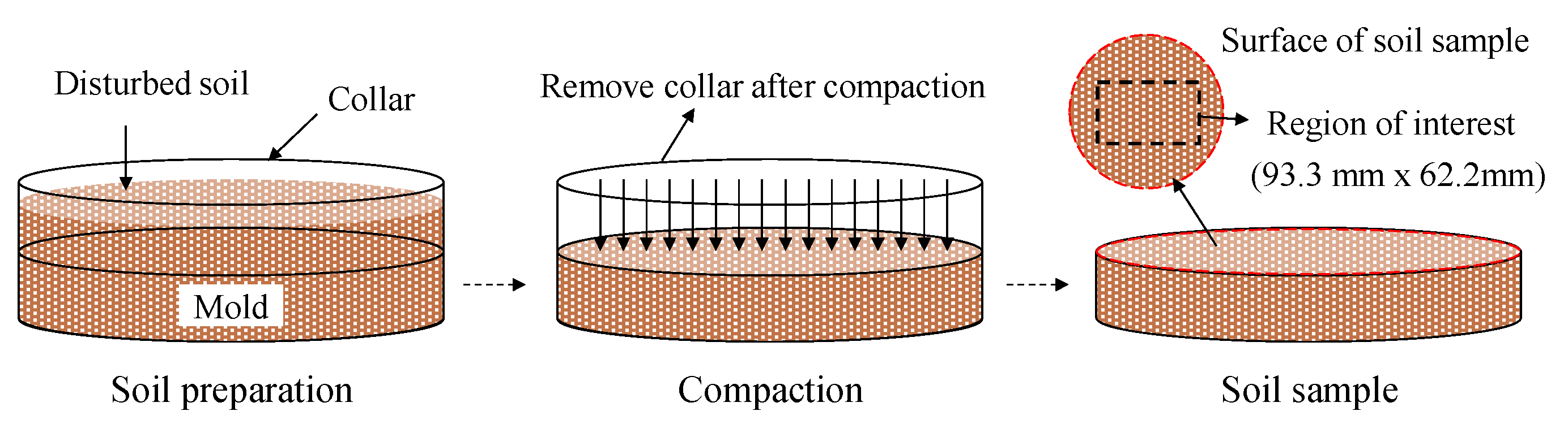
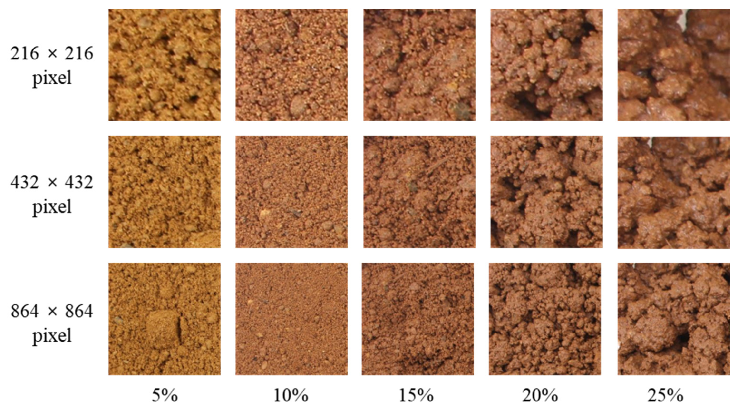
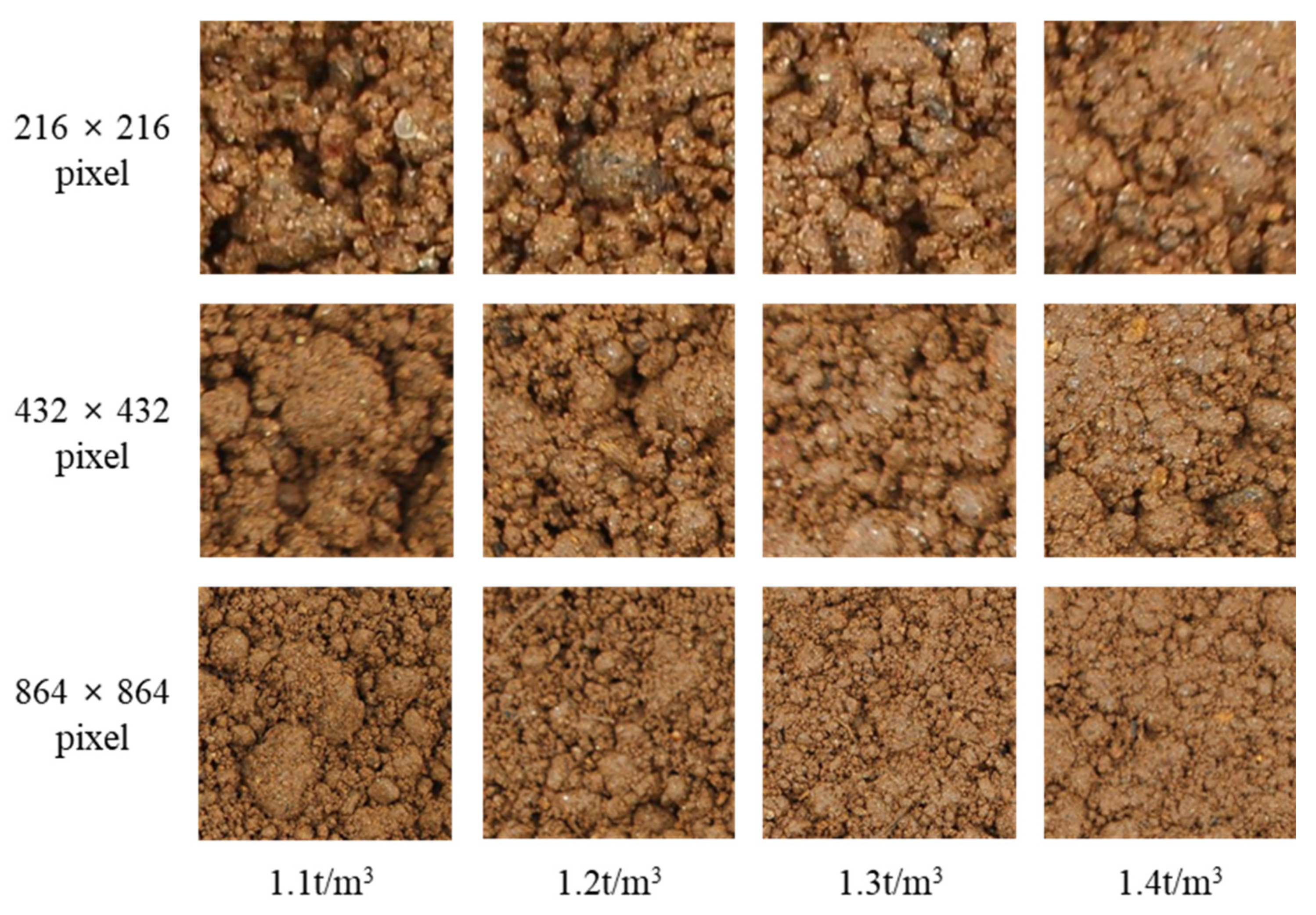
2.1. Soil Surface Image Acquisition

Soil samples were prepared in molds, and digital images of the soil surface were acquired in an indoor studio. Four agricultural land soils collected in Korea were used for the study: sandy loam (SL), loam (L), silt loam (SiL), and silty clay loam (SiCL). Soil conditions for the soil sample were determined by considering general upland soil circumstances.

Figure 1 shows the process of soil sample preparation. The soil molds were cylindrical acrylic molds, 150 mm in diameter and 50 mm in height. After oven (Changshin Science C-DOD3) drying at 110 ± 5 °C for 24 h, the WC of the oven dry soil was adjusted to 5, 10, 15, 20, and 25%. The wet soil was placed in a mold with a collar in a disturbed state. Each soil sample was compacted at four ${\rho }_{dry}$ conditions of 1.1, 1.2, 1.3, and 1.4 t/m³. The height of the sample after compaction was 50 mm, equal to the height of the mold.

Digital images were taken under controlled lighting. The correlated color temperature (CCT) measured at the soil sample location was 6400 K. The focal length of the digital camera (Canon EOS 100d) was fixed at 35 mm. The size of the digital image was 5184 × 3456 pixels. The photograph was taken in the vertical direction of the soil sample, and the distance between the soil surface and the image sensor of the camera was 240 mm. Under these conditions, one original image represented an area of 93.3 mm × 62.2 mm with a resolution of 0.018 mm/pixel. Each soil sample was prepared three times under the same conditions. Therefore, 60 digital images were taken for one soil under 5 conditions of WC, 4 conditions of ${\rho }_{dry}$ with 3 repetitions.

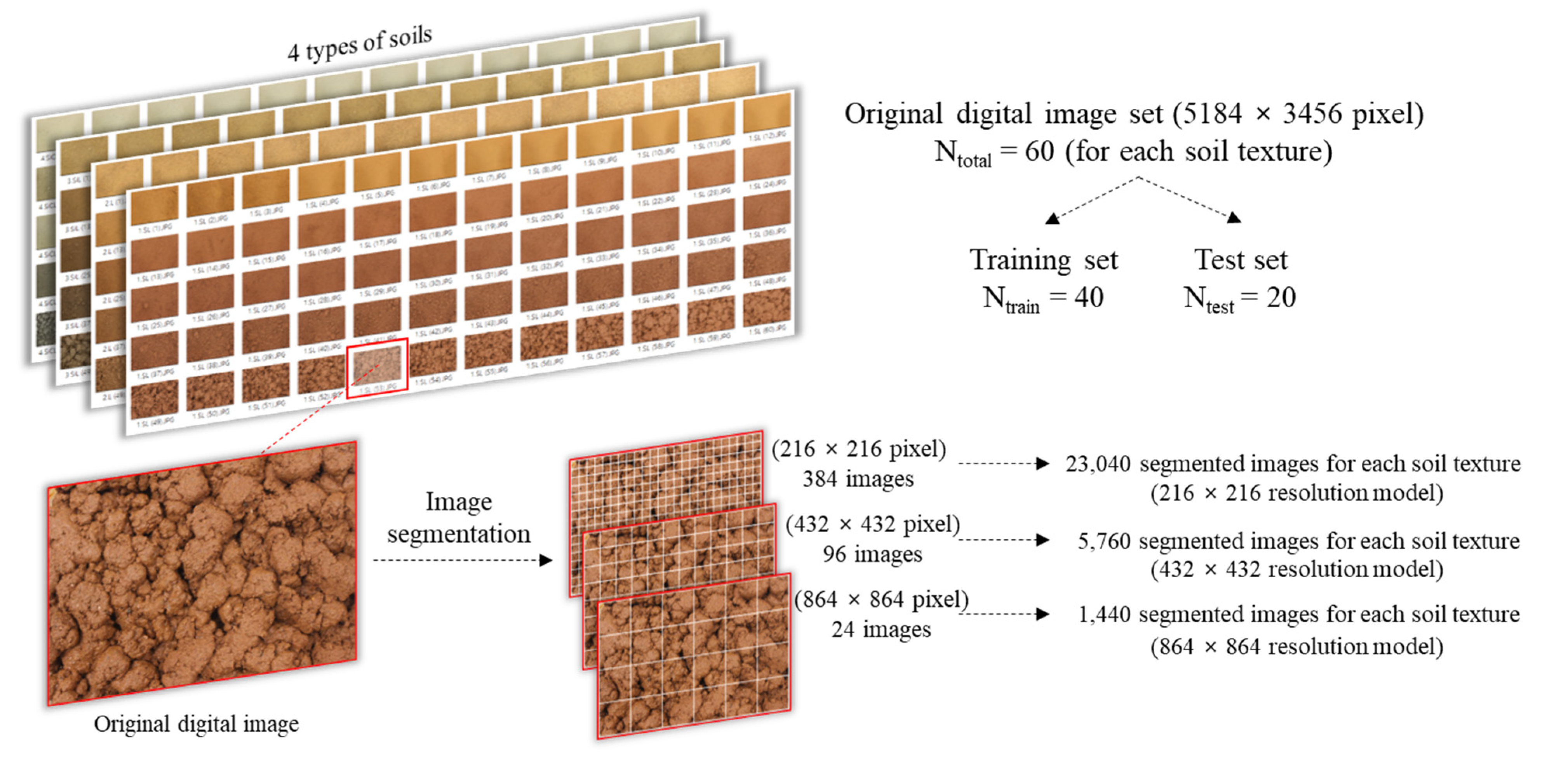
2.2. Data Preparation for the CNN Model

Figure 2 shows the input data preparation process for the CNN model. The 60 digital images for each soil texture were divided into a training set and a test set in a 2:1 ratio. Therefore, it was divided into a training set of 40 images and a test set of 20 images for each soil texture. Each digital image was divided into square-shape-segmented images. When the resolution of the segmented image is high, it has many features of the original image, but the number of images used for training becomes smaller. Conversely, when the resolution of the segmented image is low, the number of images used for training is increased although it has fewer features of the original image. Therefore, to improve the learning efficiency and accuracy, the CNN model was trained using segmented images in various resolutions, and the results were compared. The resolution of the segmented image was selected as 216 × 216, 432 × 432, and 864 × 864 pixels, respectively.

2.3. Convolutional Neural Network

In this study, a representative CNN-based image classification model based on AlexNet [10] was constructed. The model contains three convolutional layers and two fully connected layers. The program code was written in Python and used TensorFlow. CUDA and cuDNN were also used to enable GPU-based learning. The accuracy and learning efficiency of the CNN model can vary greatly depending on the value of the hyperparameter [19,20,21]. The most common method for selecting hyperparameters is trial and error or manual search [22,23,24,25]. Therefore, among the hyperparameters, epoch, batch size, learning late, and feature were determined for each model through trial and error.

In a CNN model, classification results can be obtained for each segmented image. Since a CNN model is categorical, the output value is a categorical result. Therefore, WC was output as one of five categories: 5, 10, 15, 20, and 25%. ${\rho }_{dry}$ was also output as one of four categories: 1.1, 1.2, 1.3, and 1.4 t/m³.

The classification results and the quantitative results were determined using the categorical results of the CNN model. The method for determining the classification results of the original digital image by the CNN model is shown in Figure 3. The category with the highest frequency among all segmented images was determined as the classification result of one original image.

The quantitative prediction result of the original digital image by the CNNmodel is determined by Equation (1).

$$\overline{X}=\frac{{{\displaystyle \sum }}_{i=1}^n{X}_i}{n}$$

(1)

where $\overline{X}$ is a quantitative result of CNN-model, $X_i$ is the result of i-th segment image, and n is the number of segmented images. To determine the quantitative result, the categorical result of each segment image was averaged from one original image. The accuracy of the quantitative results determined under various soil conditions was evaluated through root mean square error (RMSE). The calculation method of RMSE is shown in Equation (2).

$$RMSE=\sqrt{\frac{{{\displaystyle \sum }}_{i=1}^N{\left({\overline{X}}_i-Y_i\right)}^2}{N}}$$

(2)

where ${\overline{X}}_i$ is i-th $\overline{X}$, $Y_i$ is the actual observation value of i-th soil image, and N is the number of observations. Since there were three CNN models depending on the resolution of the segmented image, the accuracy of each model was evaluated through RMSE.

3. Results

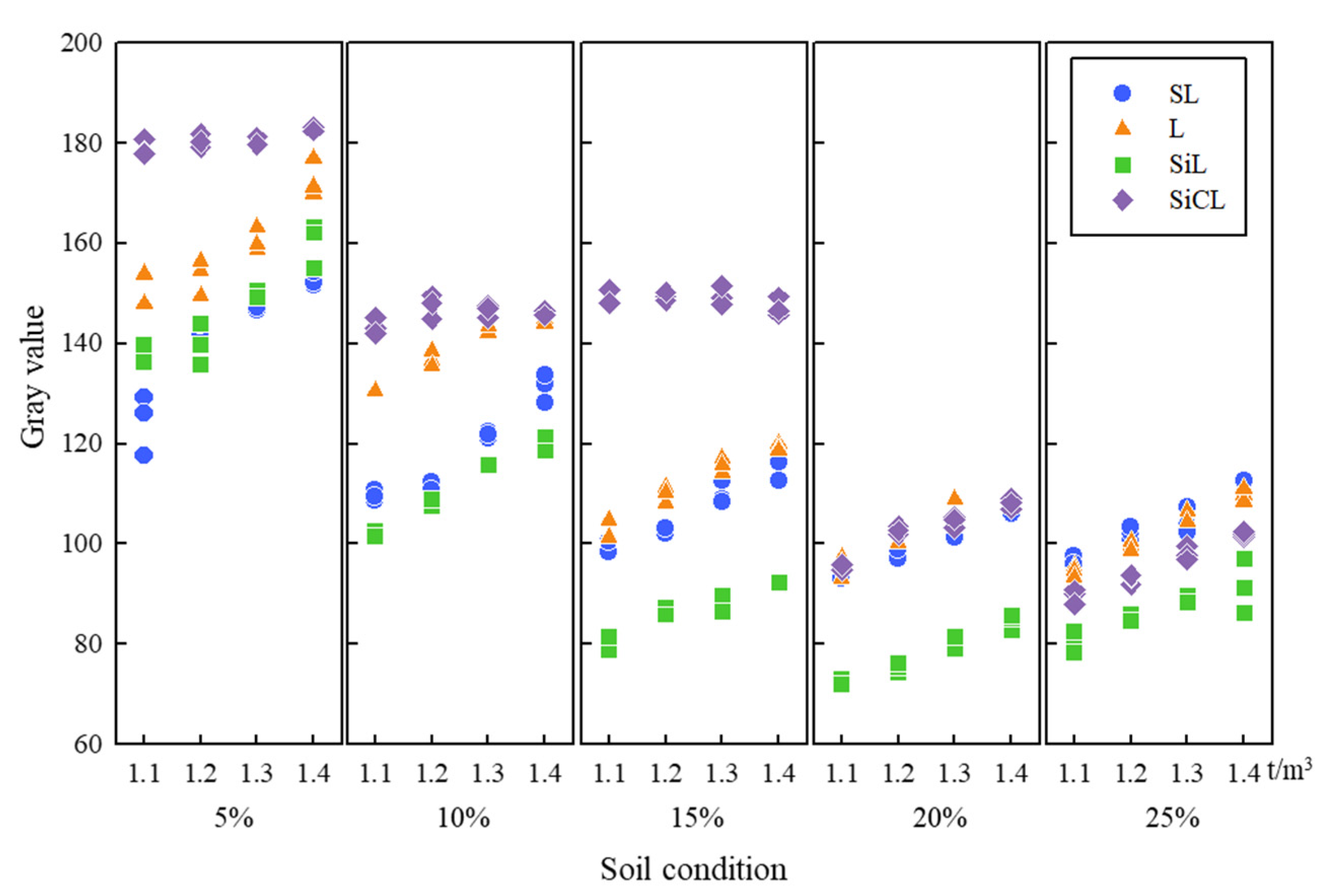
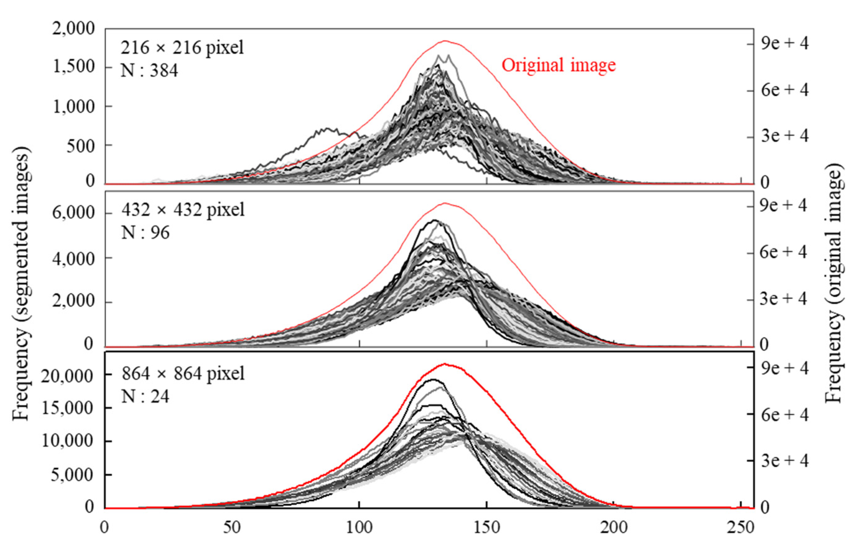
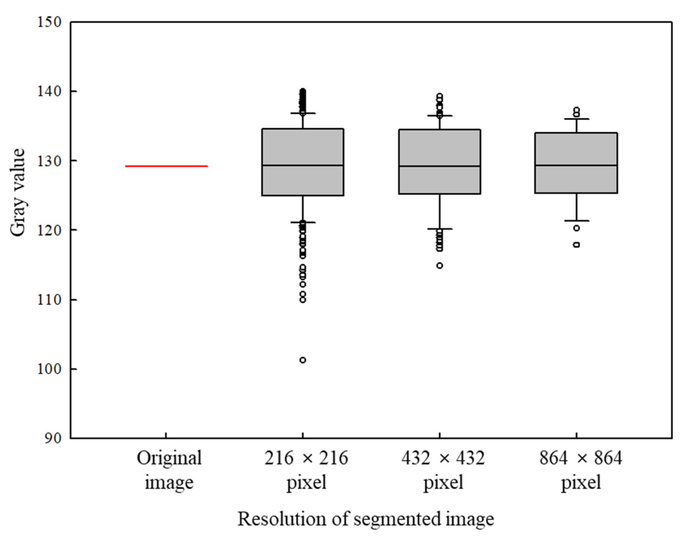
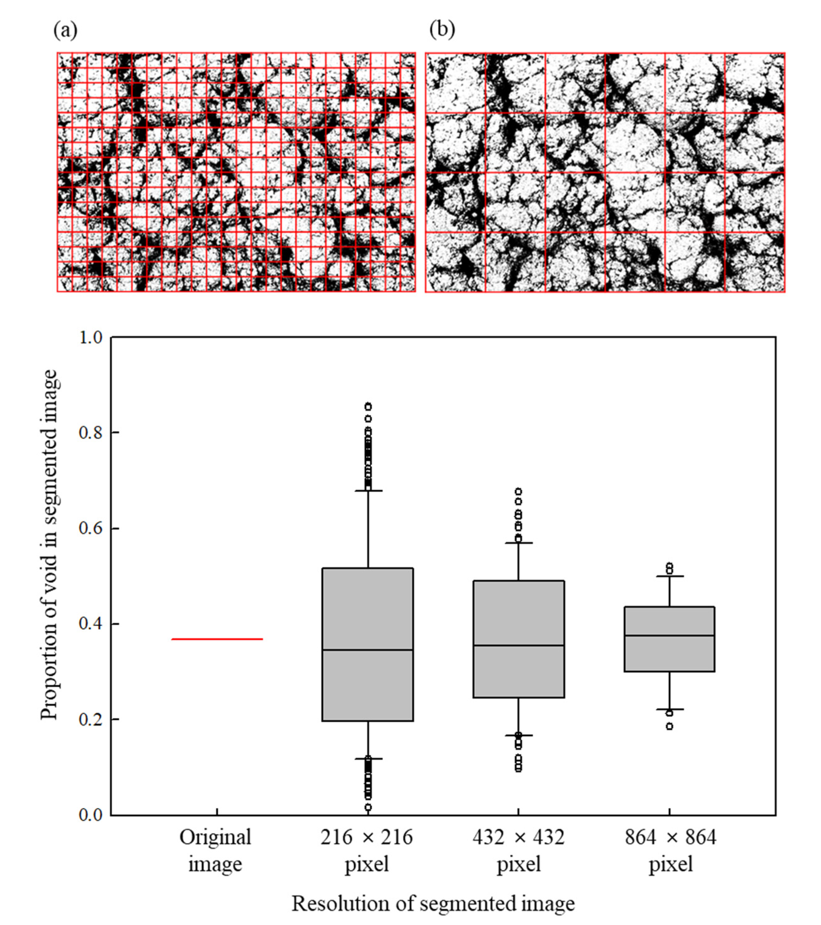
3.1. Quality of Original and Segmented Images

Figure 4 shows the gray value according to the soil conditions of 240 original images. As WC gradually increased, the gray value tended to decrease overall. When WC was high, the gray value was maintained or partially increased. This was because as soil was almost saturated, subsequent moisture came out to the soil surface and reflected light [26]. As ${\rho }_{dry}$ increased, the gray value appeared to increase. This was because the distribution of voids, which are relatively dark regions, decreased as the soil was compacted [27]. This tendency was maintained well in SL, L, and SiL with high sand content. SiCL with high clay content was found to have no significant difference in gray value change with increasing ${\rho }_{dry}$ under low WC conditions.

Sample segmented images for WC and ${\rho }_{dry}$ prediction are shown in Figure 5 and Figure 6. As WC increased, the brightness of the image decreased and the saturation increased. Additionally, the higher the WC, the more the soil became agglomerated. As ${\rho }_{dry}$ increased, the distribution of voids in the surface layer decreased. No significant color difference according to the resolution of the images was observed.

Figure 7 shows the histogram of the sample original image and the histogram of the segmented image by resolution. There were no significant differences in the peak and shape between the histograms of the original and segmented images. Therefore, the segmented images represented the color distribution of the original image well. However, outliers were observed when the resolution of the segmented images was small.

Figure 8 shows the distribution of the average gray value of the original and segmented images. The smaller the segment size, the higher the variance of the gray value, and the more outliers. As shown in Figure 4, the color of the soil was observed differently depending on WC and ${\rho }_{dry}$. Therefore, if the variance of image color increased, the prediction of WC and ${\rho }_{dry}$ may have been adversely affected. However, since a CNN model learns by finding the features of the image by itself, it may succeed in predicting based on other features of the image as well as soil color.

Figure 9 shows the difference of void distribution among the segmented images. The distribution of voids is a factor closely related to soil dry density. The original image used to analyze the void distribution in Figure 9 had a texture of SL and a soil condition of 25% WC and ${\rho }_{dry}$ of 1.3 t/m³. To confirm the void distribution of the original image, the original image was converted to grayscale, and thresholding was performed with the Otsu thresholding method to obtain a binary image divided into soil solid and void. In the binary image, it was assumed that white represented soil solid and black represented a void. In the original image, 37% of the entire area was evaluated as a void. Comparing voids for each resolution, the more it was divided, the larger the variation of voids. Comparing (a) and (b) of Figure 9, each segment included soil solid and void evenly in (b), but it was not even in (a). Similar to the color of an image, the high variance of the void distribution in segmented images could adversely affect the accuracy of the model. However, segmented images with small resolution could show high model accuracy because the amount of training data was relatively large.

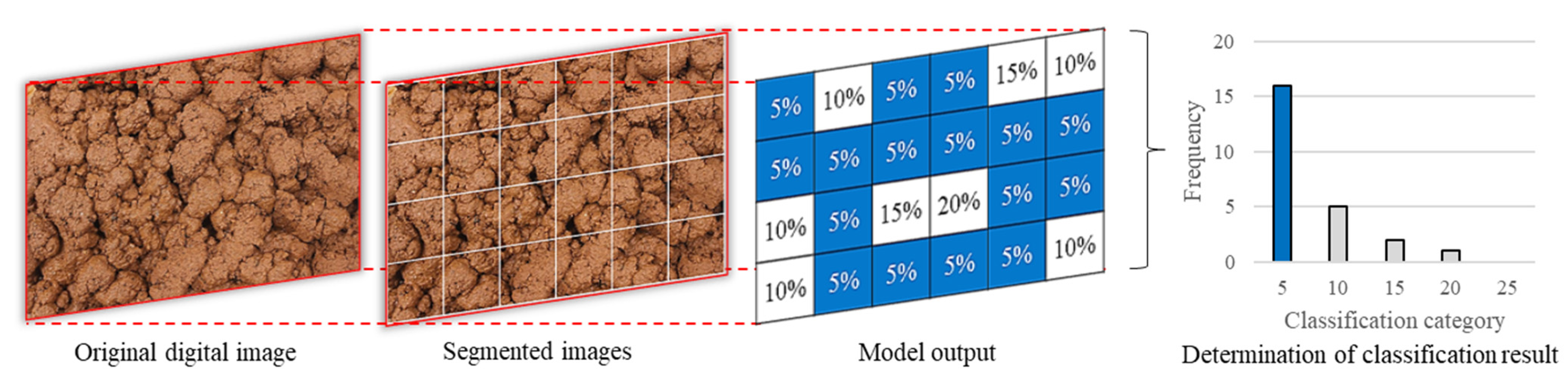
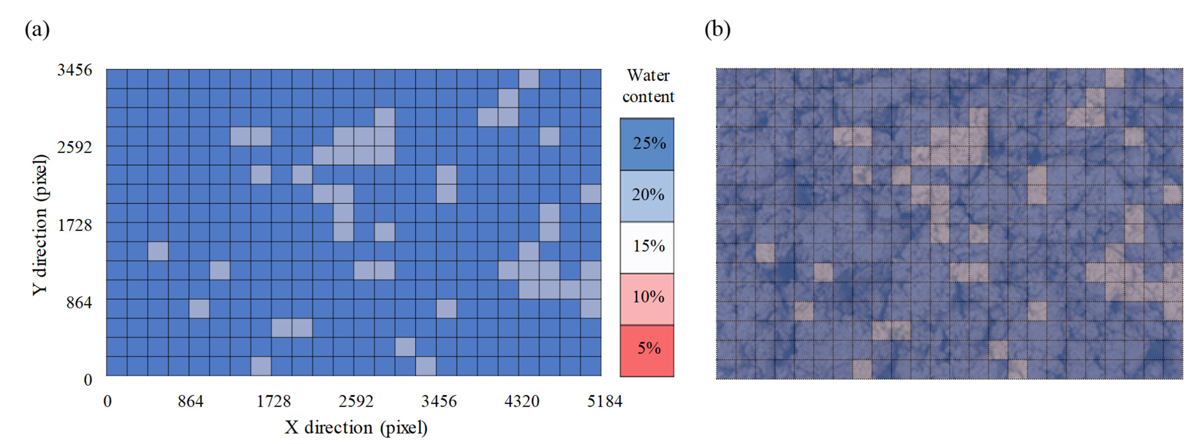
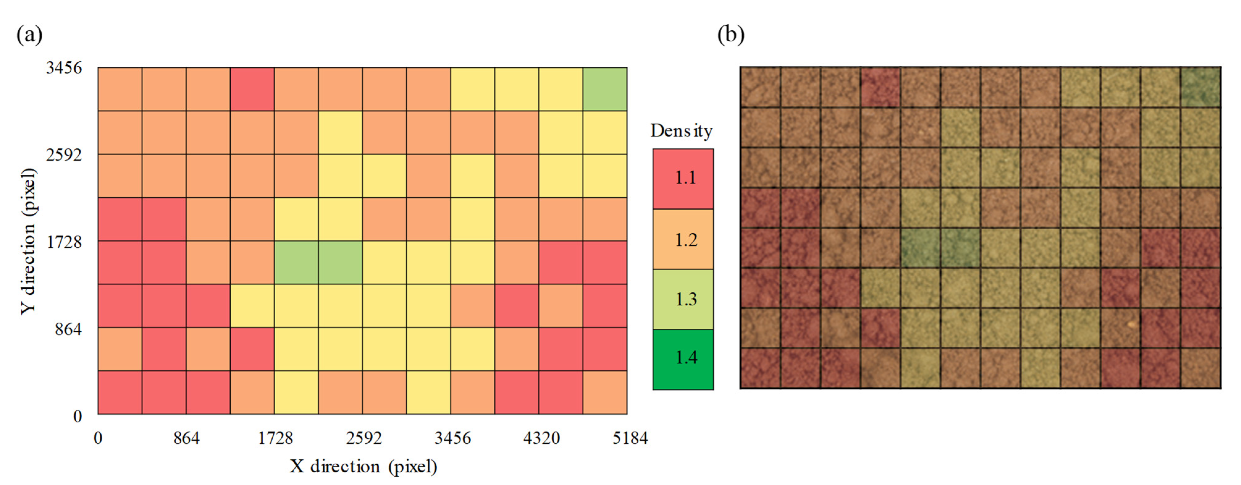
3.2. Output of CNN Model

Figure 10 and Figure 11 show an example result CNN model for prediction of WC and ${\rho }_{dry}$. In Figure 10, one original image was divided into 384 segmented images with 216 × 216 resolution and input to the model, and 384 classification results were obtained accordingly. Since it was a WC prediction model, the classification result was output as one of five classifications: 5, 10, 15, 20, and 25%. In the case of Figure 10, WC of the original soil was 25%, and 336 out of 384 segmented images were classified as 25%, and 48 were classified as 20%. Here, 25% of WC, which accounted for 336 of 384, was the WC classification result using the CNN model. The quantitative result of WC prediction was 24.4% by Equation (1).

An example of the results of ${\rho }_{dry}$ prediction using the CNN model was the same as in Figure 11. In the example, for ${\rho }_{dry}$ prediction, one original image was segmented into 96 images of 432 × 432 resolution and then input into the model for obtaining 96 classification results. In Figure 11, 21 of the 96 segmented images were classified as 1.1 t/m³, 43 as 1.2 t/m³, 29 as 1.3 t/m³, and 3 as 1.4 t/m³. Here, 1.2 t/m³, which accounted for 43 of the totals 96, was the classification result of the ${\rho }_{dry}$ using the CNN model.

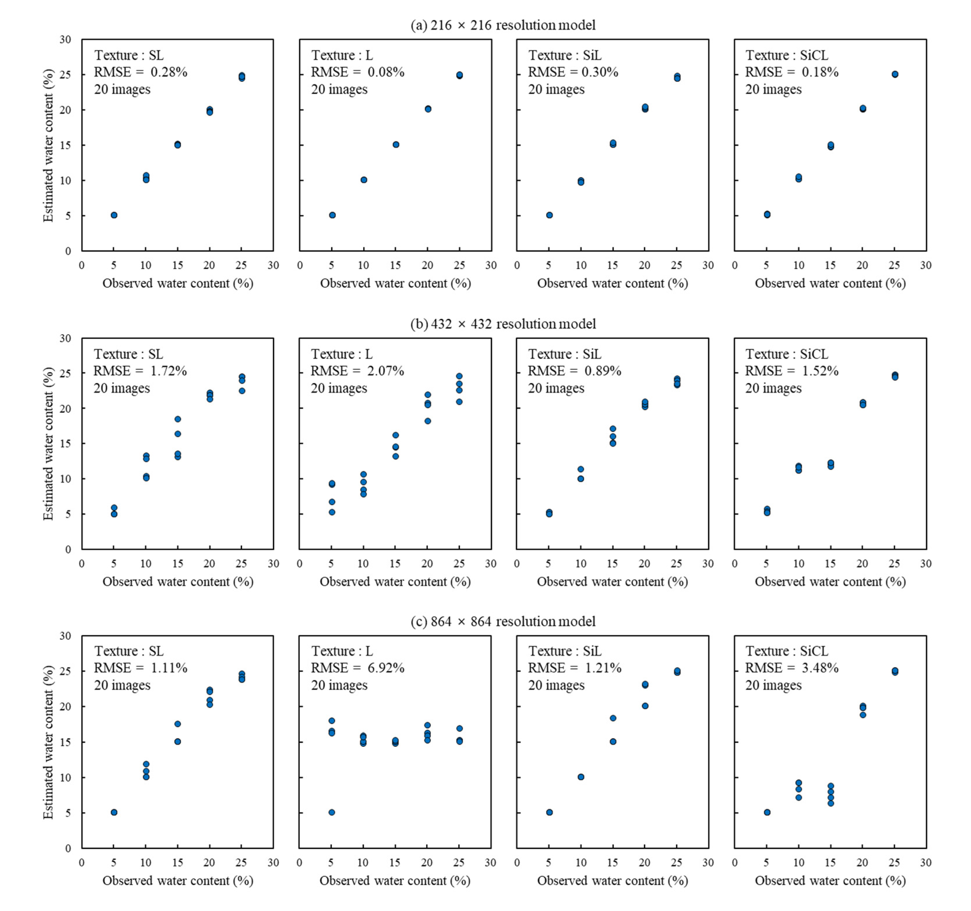
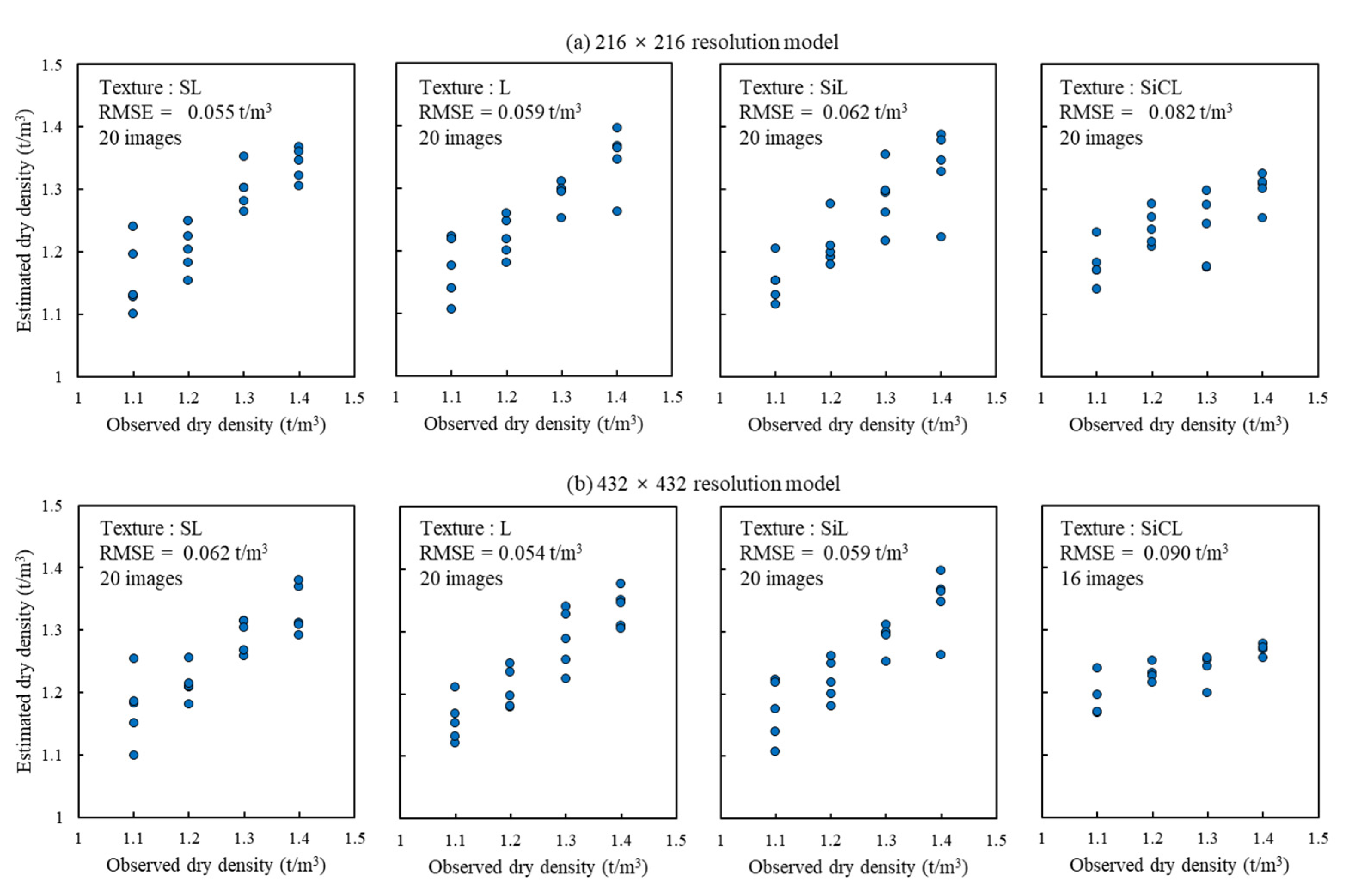
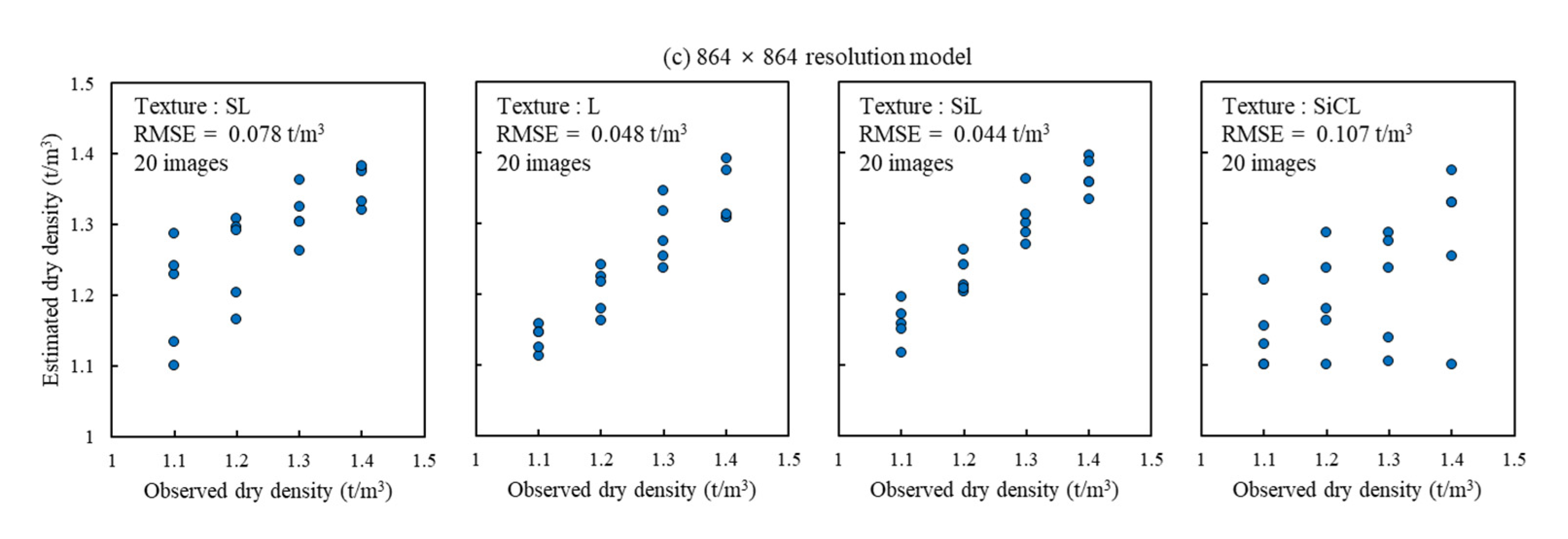
3.3. Accuuracy of Soil Water Content and Soil Dry Density Prediction

The classification accuracy of CNN model is summarized in

Table 1. Classification results by the convolutional neural network model.

Model.	Texture	Accuracy (Correct/Total)
		216 × 216 Resolution	432 × 432 Resolution	864 × 864 Resolution
WC prediction	SL	100% (20/20)	90% (18/20)	95% (19/20)
	L	100% (20/20)	100% (20/20)	35% (7/20)
	SiL	100% (20/20)	100% (20/20)	85% (17/20)
	SiCL	100% (20/20)	100% (20/20)	100% (20/20)
Overall accuracy		100% (80/80)	97.5% (78/80)	78.75% (63/80)
Dry density prediction	SL	75% (15/20)	60% (12/20)	50% (10/20)
	L	70% (14/20)	65% (13/20)	50% (10/20)
	SiL	65% (13/20)	75% (15/20)	65% (13/20)
	SiCL	60% (12/20)	37.5% (6/16)	40% (8/20)
Overall accuracy		67.5% (54/20)	60.5% (46/76)	51.3% (41/80)

. For WC prediction, the 216 × 216 resolution model had the highest classification accuracy. The 432 × 432 model also successfully classified WC under various ${\rho }_{dry}$ conditions with a total accuracy of 97.5%. The 864 × 864 model showed total accuracy of 78.75%, which is relatively low compared to that of other models. WC is highly correlated with soil color [28,29,30,31,32,33]. We confirmed that color differences due to resolution were not significant in the segmented images of the training set. Therefore, the 216 × 216 resolution model with a larger training set size was considered to have the highest accuracy. Specifically, the model’s strong point was its ability to predict WC with high accuracy under various soil dry density conditions.

The ${\rho }_{dry}$ model also showed the highest accuracy with the 216 × 216 resolution model, similarly to the results of the WC prediction model. The resolution of each image was 0.018 mm/pixel. Thus, a 216 × 216 pixel-segmented image represented an actual area of approximately 3.9 mm × 3.9 mm. The CNN model was deemed to have learned the void features by itself and predicted ${\rho }_{dry}$ even for small area-segmented images. The classification result of the ${\rho }_{dry}$ prediction model showed relatively low classification accuracy compared to that of the WC prediction model. This was expected to appear due to the difference in the natural properties of WC and ${\rho }_{dry}$. WC has a strong correlation with soil color, while ${\rho }_{dry}$ is governed by the distribution of voids. There was no significant difference in soil color in the segmented images, but the distribution of voids could be prominent in some segmented images and barely appear in others. Accordingly, it was considered that the classification accuracy of ${\rho }_{dry}$ was relatively low.

Figure 12 and Figure 13 show the quantitative results by the CNN models. In Figure 12, the RMSEs of the WC quantitative results were 0.18 to 0.30, 0.89 to 2.07, and 1.11 to 3.48%, respectively. Same as the classification accuracy, the accuracy of the 216 × 216 resolution model was the highest. Compared to that of the 216 × 216 resolution model, the 432 × 432 resolution model showed a large deviation in predicted values, resulting in a relatively high RMSE. In the case of the 864 × 864 resolution model, the RMSE increased compared to that of the 432 × 432 resolution model, and many outliers were observed. Therefore, it was considered desirable to use a 216 × 216 resolution model.

In Figure 13, the RMSEs of the prediction results were 0.055 to 0.082, 0.054 to 0.090, and 0.044 to 0.107 t/m³, respectively. Similar to the WC model, the accuracy of the 216 × 216 resolution model was the highest. Although the classification accuracy of ${\rho }_{dry}$ prediction was low, relatively stable prediction results were derived when RMSE was calculated by calculating quantitative values. Therefore, it was considered that it was preferable to use a quantitative result rather than a classification result for the prediction of ${\rho }_{dry}$.

4. Discussion

In this study, a CNN model was adopted as a method to predict WC and ${\rho }_{dry}$ using soil surface images. Study results showed that the CNN model successfully performed the training and could predict WC and ${\rho }_{dry}$ through soil surface images. The segmented images came in three sizes: 216 × 216, 432 × 432, and 864 × 864 pixels, which represented 3.9 × 3.9, 7.8 × 7.8, and 15.6 × 15.6 mm², respectively. Because color differences due to segmented image size were not large, the prediction of WC became more accurate the larger the amount of training data. Even in the case of ${\rho }_{dry}$ prediction, the overall accuracy was high if there was a lot of training data, but it was not overwhelmingly superior as in the WC model. In the case of soil texture of L and SiL, the accuracy of the 864 × 864 resolution model was the best, and in the case of soil texture of L and SiCL, the accuracy of the 216 × 216 resolution model was the highest. This was expected because the difference in void distribution between segmented images was larger than that of color.

According to Brewer’s [34] pore-size classification, soil pores are divided into macropores, mesopores, micropores, etc. Macropores are pores with an equivalent diameter of 0.075 mm or greater. Macropores are pores in which crop roots can easily grow and are those that are most significantly reduced by compaction [35,36]. Thus, macropores have the highest correlation with soil dry density. Macropores are divided into subclasses according to size, such as coarse (>5 mm), medium (2–5 mm), fine (1–2 mm), and very fine (0.075–1 mm). By comparing the size of macropores and segmented images, those segmented images with a 216 × 216 resolution can be represented on the image up to fine macropores. However, the ${\rho }_{dry}$ prediction model of 216 × 216 resolution showed a higher overall performance than other models did. This was because the 216 × 216 model had four times more training data than the 432 × 432 model and 16 times more than the 864 × 864 model did. Thus, although the 216 × 216 model was the most accurate in the current results, it is expected that the accuracy of other models would become better with additional training data. Furthermore, as the size of the segmented image increases, the model is expected to become more general, as more features of pore distribution can be included in the image.

We examined whether a general CNN algorithm could learn the features of soil surface images and consequently predict soil properties. As new deep learning algorithms are continuously being developed, the accuracy of soil image analysis and feature prediction techniques using deep learning is predicted to increase. However, as in the results of this study, the amount of training data has a great influence on accuracy. Most surface images of soil on the internet cannot be used as training data because the shooting conditions are different and there are no data on soil characteristics. Therefore, securing a good soil image database for deep learning is considered a priority for future research.

We proposed a CNN model that can predict soil moisture and soil dry density with a soil surface image. The advantage of the proposed method is that it is accessible because it uses a commercial-level camera, which is currently the most widespread sensor. Additionally, there is no need to purchase a specific purpose sensor. This can be a great strength in the field of agricultural land and field-scale water resource management.

The results of this study enable detailed agricultural land observation compared to remote sensing, which aims to observe large areas. However, it is difficult to manually acquire surface soil images of many points of interest. Tractors, which are essential in farmland, have recently been equipped with camera systems for autonomous driving and field management [37]. If a camera for surface soil observation is added to the tractor’s camera system, a larger area can be monitored using the results of this study. In addition, since this study targeted surface soil images, there is a practical limitation for observing in deep soil layers. Accordingly, verification using deep soil surface images obtained after removing the surface layer or images obtained using borehole imaging will be necessary in future studies.

5. Conclusions

This paper proposes CNN models to predict WC and ${\rho }_{dry}$ using surface images of soil and presents a digital image processing procedure for training data construction. The original image was segmented with various resolutions and used as training data for the CNN model. Proper image segmentation increased the number of training data and enabled prediction of WC and ${\rho }_{dry}$ even with few original images. The results showed excellent classification and quantitative results in predicting WC. Classification accuracy in ${\rho }_{dry}$ prediction was relatively low, but quantitative results showed that ${\rho }_{dry}$ was predicted well. In the segmented image, the range of colors and voids that could significantly affect WC and ${\rho }_{dry}$ increased compared to that in the original image, but the CNN algorithm learned features in the soil surface by itself and successfully predicted WC and ${\rho }_{dry}$.

The resolution of the original images used in this study was fixed at 0.018 mm/pixel. It is expected that the accuracy of the model would vary with the resolution of the original image. Increasing the distance per pixel may represent a larger area but may not clearly reveal detailed features of the soil surface. Future research should take this into account when determining the appropriate resolution for deep learning training data.

Additionally, the most fundamental form of the CNN algorithm was applied in this study. The reason for this was to determine whether the most common form of the CNN algorithm could learn the features of soil images. The results showed that learning was successful. Therefore, it is predicted that the application of various CNN algorithms currently being developed will greatly increase the accuracy of the model. However, as mentioned above, the construction of a good soil surface image database must precede.

References

1. Qafoku, N.P. Climate-change effects on soils: Accelerated weathering, soil carbon, and elemental cycling. Adv. Agron. 2015, 131, 111–172. [Google Scholar]
2. Shani, U.; Dudley, L. Field studies of crop response to water and salt stress. Soil Sci. Soc. Am. J. 2001, 65, 1522–1528. [Google Scholar] [CrossRef]
3. Keller, T.; Håkansson, I. Estimation of reference bulk density from soil particle size distribution and soil organic matter content. Geoderma 2010, 154, 398–406. [Google Scholar] [CrossRef]
4. Mat, I.; Kassim, M.R.M.; Harun, A.N.; Yusoff, I.M. IoT in precision agriculture applications using wireless moisture sensor network. In Proceedings of the 2016 IEEE Conference on Open Systems (ICOS), Langkawi, Malaysia, 10–12 October 2016; pp. 24–29. [Google Scholar]
5. Ge, Y.; Thomasson, J.A.; Sui, R. Remote sensing of soil properties in precision agriculture: A review. Front. Earth Sci. 2011, 5, 229–238. [Google Scholar] [CrossRef]
6. Bengio, Y.; Courville, A.; Vincent, P. Representation learning: A review and new perspectives. IEEE Trans. Pattern Anal. Mach. Intell. 2013, 35, 1798–1828. [Google Scholar] [CrossRef] [Green Version]
7. Zatarain Cabada, R.; Rodriguez Rangel, H.; Barron Estrada, M.L.; Cardenas Lopez, H.M. Hyperparameter optimization in CNN for learning-centered emotion recognition for intelligent tutoring systems. Soft Comput. 2020, 24, 7593–7602. [Google Scholar] [CrossRef]
8. LeCun, Y.; Boser, B.; Denker, J.S.; Henderson, D.; Howard, R.E.; Hubbard, W.; Jackel, L.D. Backpropagation applied to handwritten zip code recognition. Neural Comput. 1989, 1, 541–551. [Google Scholar] [CrossRef]
9. LeCun, Y.; Bottou, L.; Bengio, Y.; Haffner, P. Gradient-based learning applied to document recognition. Proc. IEEE 1998, 86, 2278–2324. [Google Scholar] [CrossRef] [Green Version]
10. Krizhevsky, A.; Sutskever, I.; Hinton, G.E. Imagenet classification with deep convolutional neural networks. Commun. ACM 2017, 60, 84–90. [Google Scholar] [CrossRef] [Green Version]
11. Szegedy, C.; Liu, W.; Jia, Y.; Sermanet, P.; Reed, S.; Anguelov, D.; Erhan, D.; Vanhoucke, V.; Rabinovich, A. Going deeper with convolutions. In Proceedings of the IEEE Conference on Computer Vision and Pattern Recognition, Boston, MA, USA, 7–12 June 2015; pp. 1–9. [Google Scholar]
12. He, K.; Zhang, X.; Ren, S.; Sun, J. Deep residual learning for image recognition. In Proceedings of the IEEE Conference on Computer Vision and Pattern Recognition, Las Vegas, NV, USA, 27–30 June 2016; pp. 770–778. [Google Scholar]
13. Huang, G.; Liu, Z.; Van Der Maaten, L.; Weinberger, K.Q. Densely connected convolutional networks. In Proceedings of the Proceedings of the IEEE Conference on Computer Vision and Pattern Recognition; Honolulu, HI, USA, 21–26 July 2017, pp. 4700–4708.
14. Veres, M.; Lacey, G.; Taylor, G.W. Deep learning architectures for soil property prediction. In Proceedings of the 2015 12th Conference on Computer and Robot Vision, Halifax, NS, Canada, 3–5 June 2015; pp. 8–15. [Google Scholar]
15. Masri, D.; Woon, W.L.; Aung, Z. Soil property prediction: An extreme learning machine approach. In Proceedings of the International Conference on Neural Information Processing, Montreal, QC, Canada, 7–12 December 2015; pp. 18–27. [Google Scholar]
16. You, J.; Li, X.; Low, M.; Lobell, D.; Ermon, S. Deep gaussian process for crop yield prediction based on remote sensing data. In Proceedings of the Thirty-First AAAI Conference on Artificial Intelligence, San Francisco, CA, USA, 4–9 February 2017. [Google Scholar]
17. Padarian, J.; Minasny, B.; McBratney, A.B. Using deep learning for digital soil mapping. Soil 2019, 5, 79–89. [Google Scholar] [CrossRef] [Green Version]
18. Srisutthiyakorn, N. Permeability Prediction of 3-D Binary Segmented Images using Neural Networks. In SEG Technical Program Expanded Abstracts; Society of Exploration Geophysicists: Houston, YX, USA, 2016. [Google Scholar]
19. Guo, Y.; Li, J.-Y.; Zhan, Z.-H. Efficient hyperparameter optimization for convolution neural networks in deep learning: A distributed particle swarm optimization approach. Cybern. Syst. 2020, 52, 36–57. [Google Scholar] [CrossRef]
20. Monshi, M.M.A.; Poon, J.; Chung, V.; Monshi, F.M. CovidXrayNet: Optimizing data augmentation and CNN hyperparameters for improved COVID-19 detection from CXR. Comput. Biol. Med. 2021, 133, 104375. [Google Scholar] [CrossRef]
21. Zhang, M.; Li, H.; Pan, S.; Lyu, J.; Ling, S.; Su, S. Convolutional neural networks-based lung nodule classification: A surrogate-assisted evolutionary algorithm for hyperparameter optimization. IEEE Trans. Evol. Comput. 2021, 25, 869–882. [Google Scholar] [CrossRef]
22. Bergstra, J.; Bengio, Y. Random search for hyper-parameter optimization. J. Mach. Learn. Res. 2012, 13, 281–305. [Google Scholar]
23. Mortazi, A.; Bagci, U. Automatically designing CNN architectures for medical image segmentation. In Proceedings of the International Workshop on Machine Learning in Medical Imaging, Granada, Spain, 16 September 2018; pp. 98–106. [Google Scholar]
24. Smith, L.N. A disciplined approach to neural network hyper-parameters: Part 1--learning rate, batch size, momentum, and weight decay. arXiv 2018, arXiv:1803.09820. [Google Scholar]
25. Xiao, X.; Yan, M.; Basodi, S.; Ji, C.; Pan, Y. Efficient hyperparameter optimization in deep learning using a variable length genetic algorithm. arXiv 2020, arXiv:2006.12703. [Google Scholar]
26. Park, J.S. Soil Classification and Characterization Using Unmanned Aerial Vehicle and Digital Image Processing. Ph.D. Thesis, Seoul National University, Seoul, Republic of Korea, 2017. [Google Scholar]
27. Lucas, M.; Schlüter, S.; Vogel, H.-J.; Vetterlein, D. Roots compact the surrounding soil depending on the structures they encounter. Sci. Rep. 2019, 9, 16236. [Google Scholar] [CrossRef] [PubMed] [Green Version]
28. Persson, M. Estimating surface soil moisture from soil color using image analysis. Vadose Zone J. 2005, 4, 1119–1122. [Google Scholar] [CrossRef]
29. Zhu, Y.; Wang, Y.; Shao, M. Using soil surface gray level to determine surface soil water content. Sci. China Earth Sci. 2010, 53, 1527–1532. [Google Scholar] [CrossRef]
30. Gómez-Robledo, L.; López-Ruiz, N.; Melgosa, M.; Palma, A.J.; Capitán-Vallvey, L.F.; Sánchez-Marañón, M. Using the mobile phone as Munsell soil-colour sensor: An experiment under controlled illumination conditions. Comput. Electron. Agric. 2013, 99, 200–208. [Google Scholar] [CrossRef]
31. Zanetti, S.S.; Cecílio, R.A.; Alves, E.G.; Silva, V.H.; Sousa, E.F. Estimation of the moisture content of tropical soils using colour images and artificial neural networks. Catena 2015, 135, 100–106. [Google Scholar] [CrossRef]
32. Dos Santos, J.F.; Silva, H.R.; Pinto, F.A.; Assis, I.R.d. Use of digital images to estimate soil moisture. Rev. Bras. De Eng. Agrícola E Ambient. 2016, 20, 1051–1056. [Google Scholar] [CrossRef]
33. Kim, D.; Son, Y.; Park, J.; Kim, T.; Jeon, J. Evaluation of calibration method for field application of UAV-based soil water content prediction equation. Adv. Civ. Eng. 2019, 2019, 2486216. [Google Scholar] [CrossRef] [Green Version]
34. Brewer, R. Fabric and Mineral Analysis of Soils; John Wiley and Sons: New York, NY, USA, 1964. [Google Scholar]
35. Van den Akker, J.; Soane, B. Compaction. In Encyclopedia of Soils in the Environment; Hillel, D., Ed.; Elsevier: Oxford, UK, 2005; pp. 285–293. [Google Scholar]
36. Ruser, R.; Sehy, U.; Weber, A.; Gutser, R.; Munch, J. Main driving variables and effect of soil management on climate or ecosystem-relevant trace gas fluxes from fields of the FAM. In Perspectives for Agroecosystem Management; Elsevier: Amsterdam, The Netherlands, 2008; pp. 79–120. [Google Scholar]
37. Vrochidou, E.; Oustadakis, D.; Kefalas, A.; Papakostas, G.A. Computer vision in self-steering tractors. Machines 2022, 10, 129. [Google Scholar] [CrossRef]
Figure 1. Soil sample preparation process for digital image acquisition of soil surface layer.
Applsci 13 02936 g001
Figure 2. Training and test data preparation process for the convolutional neural network model.
Applsci 13 02936 g002
Figure 3. Classification result determination method by the convolutional neural network model.
Applsci 13 02936 g003
Figure 4. Gray value of original soil surface images according to soil texture, soil water content and soil dry density.
Applsci 13 02936 g004
Figure 5. Sample segmented soil surface images under different soil water content conditions. Each image is a cropped image with 3 different sizes from the original soil surface image with a resolution of 5184 × 3456 pixels. Soil texture is sandy loam.
Applsci 13 02936 g005
Figure 6. Sample segmented soil surface images under different soil dry density conditions. Each image is a cropped image with 3 different sizes from the original soil surface image with resolution of 5184 × 3456 pixels. Soil texture is loam.
Applsci 13 02936 g006
Figure 7. Gray value histogram of soil surface images. The solid red line is a histogram of the original soil surface image, and the solid grayscale lines are histograms of segmented images. N is the number of segmented images and its histograms.
Applsci 13 02936 g007
Figure 8. Distribution of average gray value of soil surface images. The solid red line is the average gray value of the original image, and the number of segmented images for each resolution was 384, 96, and 24, respectively.
Applsci 13 02936 g008
Figure 9. Difference in void distribution among segmented images. (a) is the binary image divided 216 into 384 segmented images of 216 × 216 pixels. (b) is the binary image divided into 24 segmented 217 images of 216 × 216 pixels. Black pixels in (a,b) represent the void. The solid red line in the graph is the average gray value of the original image, and the number of segmented images for each resolution was 384, 96, and 24, respectively.
Applsci 13 02936 g009
Figure 10. Example of soil water content prediction by the convolutional neural network model. (a) Classification result with a resolution of 216 × 216 segmented images.; (b) original image overlaid with classification result.
Applsci 13 02936 g010
Figure 11. Example of soil dry density prediction by the convolutional neural network model. (a) Classification result with a resolution of 432 × 432 segmented images.; (b) original image overlaid with classification result.
Applsci 13 02936 g011
Figure 12. Quantitative results of soil water content prediction by the convolutional neural network model.
Applsci 13 02936 g012
Figure 13. Quantitative results of soil dry density prediction by the convolutional neural network model.
Applsci 13 02936 g013aApplsci 13 02936 g013b