The Hydrological Balance in Micro-Watersheds Is Affected by Climate Change and Land Use Changes

Abstract

Temperate forests are key to the balance and provision of hydrological and environmental services. Currently, these forests are subject to human alterations as well as to the effects of global change, including warming, variability, deforestation, and forest fires. As a consequence, the hydrological balance has been modified. The present study simulates the effects of climate change and land use change on the hydrological balance of micro-watersheds in Mexico using the hydrological model Water Evaluation and Planning (WEAP). The land use change between 1995 and 2021 was estimated to establish a baseline. Climate scenario SSP585 was projected using three global models, MPI-ESM1-2-LR, HadGEM3-GC31-LL, and CNRM-CM6-1 by the 2081–2100 horizon, along with two scenarios of land use change: one with forest permanence and another with loss of forest cover and increased forest fires. Results indicate that future climatic conditions will modify the hydrological balance at the microbasin level. Even with positive conditions of forest permanence, increases in surface runoff of 124% (CNRM), 35% (HadGEM3), and 13% (MPI) are expected. The projections of coverage loss and fires showed surface runoff increases of 338% (CNRM), 188% (HadGEM3), and 143% (MPI). In the high areas of the microbasins where temperate forest predominates, climatic variations could be contained. If the forest is conserved, surface runoff decreases by −70% (CNRM), −87% (HadGEM3), and −89% (MPI). Likewise, the moisture in the soil increases. In areas with temperate forests, there will be modifications of the hydrological balance mainly due to the increase in evapotranspiration (due to the increase in temperature and precipitation). This will cause a significant decrease in flow and interflow. The alteration of these flows will decrease water availability in soil for infiltration. It is expected that the availability of hydrological and environmental services will be compromised in the entire study area due to climate change.

1. Introduction

Temperate forests provide numerous ecosystem benefits, but among them, hydrological provision and regulation stand out. In watersheds with forest cover, trees ensure the continuous flow of the hydrological cycle [1]. The forest is the layer of the earth’s surface responsible for the capture and buffering of rainfall, the control of surface runoff processes, the promotion of water infiltration, and the influence on the recharging of aquifers in order to maintain stable levels, among other functions [2,3,4]. However, the capacity of a basin to provide hydrological services also depends on climatology, land use, and topographic characteristics [5,6].

Despite their importance, the current capacity of ecosystems for the provision of hydrological services is in decline [7] since they are subject to alterations and effects of global change, the rates of change of which are increasing rapidly. According to Vitousek [8], the components of global change are (i) climate change (global warming, increased climate variability, etc.); (ii) changes in biogeochemical cycles (increased carbon emissions into the atmosphere, increased nitrogen and sulfur deposition, changes in ozone concentration, etc.); and (iii) changes in land management and use (deforestation, ecosystem fragmentation, changes in logging regime, fire management, etc.). However, the global change affects terrestrial ecosystems differently according to the type of community and the dominant factor [9].

Climate change affects water resources worldwide, particularly at the basin level [10,11,12]. The hydrological cycle will accelerate with an increase in temperature and will change evapotranspiration and precipitation [10,13,14]. The change in the distribution of the intensity and frequency of rainfall will affect the flow of surface runoff [15,16]. Temperature increases affect the structure of forests [17] and their geographical distribution [18,19], their phenological cycles [18,20], and their fecundity [21]. The ability of forests to provide ecosystem services can be severely impacted by these disturbances [22]. In addition, an increase in climate-related disturbances may exceed the ecological resilience of forests. As a result, ecosystems may be permanently altered as tipping points are crossed [22].

Changes in land use imply a loss of forest cover that alters the hydrological cycle [23,24]. These changes generate a decrease in aquifer recharge and dry bodies of water and generate intense runoff [25]. Changes in forest land use endanger the accessibility of hydrological ecosystem services [26]. The main change in land use in the study area is due to high-severity forest fires [27]. Anthropogenic action and extreme climate changes have altered the natural fire regime in several forest ecosystems, and these changes affect the health of forests, with increases in fires, pests, and forest diseases [28]. Climate changes mean that warmer and drier conditions particularly facilitate disturbances by fires, droughts, and insects, while warmer and wetter conditions increase disturbances caused by wind and pathogens [22].

For this reason, it is necessary to have a knowledge of the current and future state of water resources at the level of the hydrographic basin in Mexico [29], given the effects of global changes related to climate and land use. One of the ways to demonstrate climate change and the effects of land use changes on the availability and distribution of water resources is through scenario modeling. Scenarios are conceived and model alternative futures as a strategy to explore trajectories of change [30]. If the effects of climate change on the hydrological cycle are incorporated into these models, the models are even more effective [29]. In Mexico, applied models have been mostly related to the supply and demand of hydrological resources and climate change [15,29,31]. However, besides results with acceptable effectiveness, evidence is scant on the importance of relating the natural processes that are generated from the effects of climate change, changes in forest cover, and the provision of hydrological ecosystem services.

WEAP software was developed by SEI [32] and is a tool used for the modeling, planning, and distribution of water resources. It can be applied at a variety of scales, from a small watershed to a large watershed [33]. WEAP includes routines designed to analyze the distribution of water among different types of users from a human and ecosystem perspective; these characteristics make WEAP an ideal model for climate change studies, in which it is important to estimate changes in the water supply. (e.g., changes in projected precipitation) and in water demand (e.g., changes in demand due to changes in land use), which will produce a different hydrological balance at the basin level [32]. It solves water allocation problems at any time step using a standard linear programming model [34,35]. The WEAP tool operates under the water balance model, based on the variation of the volume of water stored in the soil, and has the ability to simulate processes such as: surface runoff, base flow, and infiltration, among others [33,36,37]. Scenarios provide a basis for decision-making, the development of adaptation strategies, and regional policies for the conservation of ecosystems and water [15,38]. The WEAP model can be adapted according to the existing data; in regions with limited data, the model can build a full hydrological representation [39].

The present research aimed to analyze the impact of land-use change and climate change on the hydrological balance of micro-watersheds in temperate forests of central Mexico. In this study, we use the classification of “micro-watershed” as the land area of less than 100 km² that drains all streams. To this end, scenarios were projected with estimates of land use change (positive and negative) and climate scenarios called shared socioeconomic pathways (SSPs 5-8.5) recently proposed in the sixth evaluation report of the Intergovernmental Panel on Climate Change [40], of three global models, MPI-ESM1-2-LR, CNRM-CM6-1, and HadGEM3-GC31-LL (CMIP6), using the WEAP hydrological model. The importance that the changes represent to the hydrological balance in the 2081–2100 time horizon was determined. This horizon was selected because it best visualizes the changes in the watersheds, given the scenarios applied.

2. Materials and Methods

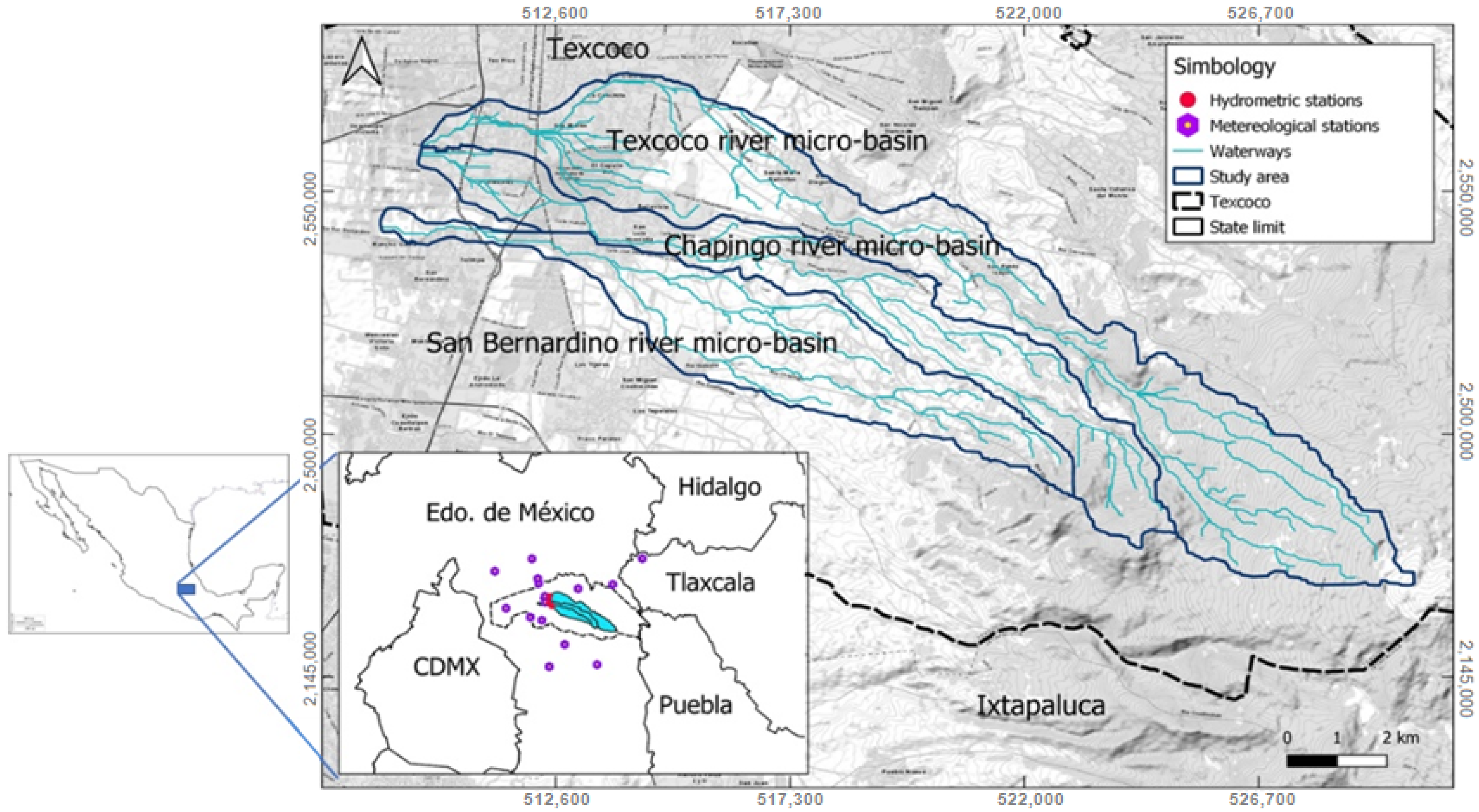
2.1. Study Area

The Chapingo, Texcoco, and San Bernardino Rivers micro-watersheds in the municipality of Texcoco, near Ciudad de Mexico, are included in the study area (Figure 1). The micro-watersheds belong to the Texcoco aquifer, which is part of the Pánuco River Hydrological Region and the “Aguas del Valle de México” Administrative Hydrological Region. This is the most densely populated region in Mexico, so its aquifers are classified as overexploited since they have an extraction volume greater than the value of their recharge [41]. The hydrographic system of the aquifer consists of torrential runoff, with short duration, and dry during the dry season [41]. The micro-watersheds are located between coordinates 509 117 and 529 827 W, 2 146 699, and 2 157 465 N. They have an average altitude gradient of 3161 m asl and cover a total land area of 77.4 km². The mean annual temperature is 11 °C and 652.5 mm of mean annual precipitation. The predominant climate according to Koeppen classification is classified as dry temperate with main rains in summer [42].

Geologically, micro-watersheds are covered mainly by sedimentary breccia material [43]. Hydrogeologically, micro-watersheds have medium to high permeability. According to INEGI [44], the type of soil with the greatest distribution is the epipetric Phaeozem. According to Ruiz-Garcia [27], in the study area, there are 10 classes of predominant land use and vegetation (

Table 1. Land use and occupied surface (hectares) in the studied micro-watersheds (based on Ruiz-García, 2022, [27]).

Land Use	Total Surface	%	Chapingo River	%	Texcoco River	%	San Bernardino River	%
Agriculture (rainfed)	2294.8	29.6	420.4	21.6	1042.8	26.7	831.6	44.2
Temperate forest	2021.4	26.1	472.1	24.2	1448.5	37.1	100.8	5.4
Reforestation	1145.6	14.8	395.4	20.3	199.9	5.1	550.3	29.2
Urban	949.9	12.3	300.0	15.4	545.9	14.0	104.0	5.5
Agriculture (irrigated)	540.3	7.0	89.1	4.6	354.6	9.1	96.7	5.1
Secondary vegetation	438.7	5.7	160.9	8.3	166.3	4.3	111.5	5.9
Mine	212.2	2.7	87.0	4.5	39.4	1.0	85.9	4.6
Agriculture (protected)	80.8	1.0	18.7	1.0	60.2	1.5	1.9	0.1
Pasture	52.2	0.7	3.6	0.2	48.6	1.2	0.1	0.0
Water	4.6	0.1	1.3	0.1	3.3	0.1	0.0	0.0
Total	7740.6	100.0	1948.5	100.0	3909.4	100.0	1882.6	100.0

Source: Own elaboration based on Ruíz-García, 2022, [27].

): rainfed agriculture (29.6%), temperate forest (26.1%), reforestation (14.8%), urban (12.3%), irrigated agriculture (7%), secondary vegetation (5.7%), mine (2.7%), protected agriculture (1%), grassland (0.7%), and water (0.1%).

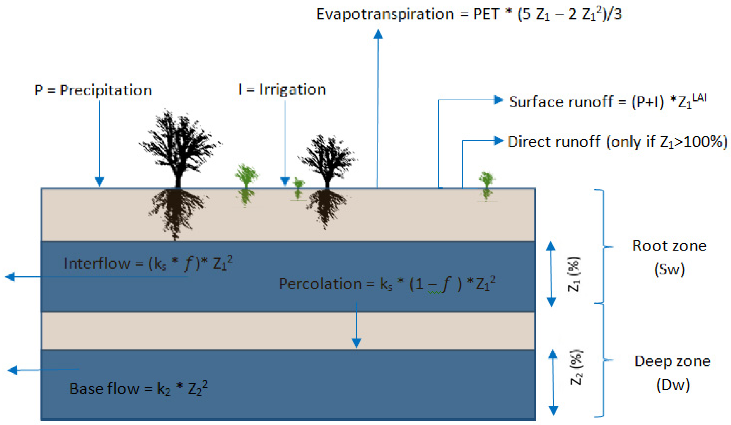
2.2. Hydrological Simulation

We chose to use WEAP because it can be used to analyze a wide range of issues that water planners face using a scenario-based approach. In addition, WEAP uses monthly data instead of daily data, which represents an advantage over models that use daily data since such robust databases are not available in the study area. WEAP has five methods to calculate the hydrological simulation, although, in this study, the soil moisture method was applied as it is the most robust of the five. The method divides the soil into two layers: root zone and deep zone, to estimate through specific functions the processes of surface runoff, evapotranspiration, interflow, base flow, and soil moisture [31,37] (Figure 2). According to Yates et al. [37], Equations (1) and (2) are used to calculate the water balance in the root zone and in the deep zone, depending on the type of coverage.

$$S{W}_j\frac{d{z}_{i,j}}{dt}=P_e\left(t\right)-PET\left(t\right)K_{cj}\left(t\right)\left(\frac{5z_{1,j}-2z_{1,j}^2}{3}\right)-P_e\left(t\right)z_{1,j}^{\frac{LA{I}_j}{2}}-f_j{k}_s{z}_{1,j}^2-\left(1-f_j\right)k_j{z}_{1,j}^2$$

(1)

$$D{w}_j\frac{d{z}_{2,j}}{dt}=\left(1-f_j\right)k_j{z}_{1,j}^2-k_2{z}_{2,j}^2$$

(2)

where: Sw_j: is the water storage capacity in the root zone (mm), z_1,j: initial moisture in the root zone (1, 0), P_e(t): effective precipitation over time (mm), PET (t): potential evapotranspiration of the reference crop (mm time⁻¹), k_c,j(t): crop coefficient over time (dimensionless), LAI_j: leaf area index (m² m⁻²), f_j: preferential flow direction (1 = 100% horizontal, 0 = 100% vertical), k_j: storage conductivity (mm time⁻¹), Dw_j: water storage capacity in the deep zone (mm) and z₂,_j: initial humidity in the deep zone (1, 0).

2.3. Data and Sources of Information

A climatic database line was established, which served as a reference to analyze the behavior of the information estimated in the simulation of scenarios. Through the download of the historical records of precipitation and monthly minimum and maximum temperature of the 15 stations closest to the micro-watersheds [43], the study area was climatically characterized by calculating isotherms and isohyets according to Gómez et al. [44]. The wind and relative humidity data were obtained from Gómez and Monterroso [45] and were classified by height, considering a historical monthly average for all the time series of the three microbasins. All weather variables were entered into the Catchments depending on their location.

2.3.1. Hydrological Catchment Units or Catchments

In WEAP, the subbasins are divided into hydrological catchment units or Catchments, which are defined by SEI [33] as basic spatial modeling units that correspond to specific catchment areas and allow to know with greater precision the value of the flow in a given area at a given time while applying the model. Following the methodology of Young et al. [46], 22 Catchments were delimited for the entire study area [27]. Through this process, specific information was obtained on the areas and distribution of the ten classes of land use and vegetation, as well as the climatological characteristics within each hydrological unit.

2.3.2. Climate Change

Within the sixth assessment report of the IPCC, the use of scenarios called SSPs that seek to incorporate the dimensions of the expected social change that could affect both the levels of emissions and the adaptation to climate change was proposed [30]. From the database of the SSPs, the information of the general circulation models (GCMs) of CMIP6 was downloaded: CNRM-CM6-1, HadGEM3-GC31-LL, and MPI-ESM1-2-LR (CMIP6, 2022) from the WorldClim page (https://www.worldclim.org/data/index.html, accessed on 25 July 2022). These models were selected because they have shown good results in other studies for the country [47,48,49]. From the GCMs, the values of the meteorological data were obtained: minimum temperature (tn), maximum temperature (tx), and precipitation (pr) for the most drastic scenarios of SSP5-8.5, with a spatial resolution of 30 s (longitude/latitude degree), this is about 900 m at the equator, which is acceptable for the size of the watershed. The data corresponded to the 2081–2100 horizon.

2.3.3. Land Use Change

Through a supervised classification, the estimation of the change in land use that the study area has suffered in the last 26 years was made. The supervised classification was developed in the QGIS software using the plugin proposed by Congedo [50] called Semi-Automatic Classification Plugin (SCP, Lansing, MI, USA) that allows downloading satellite images from the United States Geological Survey (USGS), preprocessing and postprocessing them. For this research, the chosen satellites were Landsat 5 and 8. The images correspond to the years: 1995, 2008, and 2021, with a pixel size of 30 m and with a percentage of cloud cover of less than 20%. First, the images were preprocessed using an ensemble of false-colored bands, which were used as input for classification.

According to Ruiz-Garcia [27], ten land cover classes were defined for the study area: (1) temperate forest (TF); (2) reforestation (R); (3) secondary vegetation (SV); (4) grassland (G); (5) mine (M); (6) rainfed agriculture (RA); (7) irrigated agriculture (IA); (8) protected agriculture (PA); (9) urban (U); and (10) water bodies (W). In the supervised classification, the SCP tool called Random Forest Classification [50] was used, where at least ten reconnaissance polygons were drawn per land-use class. Subsequently, a pixel-level modeling reliability report was evaluated to determine the performance of the tool, and some errors were identified and corrected by creating new reconnaissance polygons to change the value of the pixels identified as incorrect.

Through the application of the SCP tool called Land cover change, the results of the classifications of the periods 1995–2008 and 2008–2021 were compared to evaluate changes in land cover and obtain confusion matrices that quantify said changes as well as permanence of unchanged areas. Cartography was also obtained with the specific spatial location of the surfaces that have undergone some type of change in the determined time periods (Figure 3).

2.3.4. Hydrological Parameters

To calculate the hydrological balance with the soil moisture method, WEAP requires the estimation of nine land use parameters, of which six correspond to the root zone and three to the deep zone: The first one included: coefficient of crop (Kc), leaf area index (LAI), preferential flow direction (f), root zone conductivity (Ks), initial moisture of the upper layer (Z1) and water storage capacity in the root zone (Sw). The deep zone included three parameters: initial moisture of the lower layer (Z2), conductivity of the deep layer (Kd), and water storage capacity in the deep zone (Dw). For further reference, please refer to WEAP algorithm (https://www.weap21.org/WebHelp/index.html#BasicParameters.htm, accessed on 25 July 2022).

2.4. Construction of the Model

In the WEAP platform, shapefiles of land cover, microbasins, channels, centroids, and Catchments were incorporated, which served as a guide to building the model through a base scheme. Once the base scheme was created, the data structure of the Catchments was created, which included specific information for each of them, on climate data, land use parameters, and land use and vegetation classes. All land use parameters were incorporated into the model using the Key Assumptions tool, although a specific value was incorporated for each class of land use and vegetation in the root zone parameters and a single value per microbasins in the watershed parameters in the deep zone [32].

2.5. Calibration and Validation

The model was calibrated based on the coincidence between the historical precipitation series [43] and the monthly flow measurement records reported by the “National Data Bank of Surface Waters (BANDAS)” [51]. The calibration periods correspond to those reported by Ruiz-García [27]. The selection of the periods considered the continuity and extension of the records, as well as the variability of wet and dry periods. During this process, the model was fed with data on land use and vegetation for the period corresponding to 1995, which were described in Section 2.3.3 of this investigation.

In the calibration of the parameters of the hydrological balance, the sensitivity analysis proposed by Jantzen et al. [52] was used. They mention that the model is highly sensitive to changes in climate and land use parameters: precipitation, land use area, Dw, Kc, and LAI. The calibration was carried out manually, although in the calculation of the value of the parameters: Dw, f, kd, Z₁ and Z₂, the WEAP called PEST tool [32] was used to define their values with greater precision.

In the validation, the model was executed with a data period different from the one used in the calibration to determine the predictive capacity of the simulated flows, in addition to detecting any bias in the calibrated parameters [53,54]. The validation periods correspond to those reported by Ruiz-García [27]. The simulation of the calibration and validation periods was evaluated graphically to compare the simulated and observed monthly mean flows and statistically with the measurement of the goodness of fit.

Measurement of Goodness-of-Fit

Four estimators were applied [55]: the Nash-Sutcliffe efficiency or NSE, coefficient of determination or R2, the percentage bias or PBIAS, and the standard observation deviation or RSR (

Table 2. Statistics to estimate the goodness of fit of the calibration and validation.

Function	Description	Range of Values	Ecuation *
R2	It presents the linear correlation between both data series (Lu and Chiang, 2019, [55]).	0 to 1	$=\frac{{{\displaystyle \sum }}_{i=1}^n{\left(Y_i^{sim}-Y^{mean}\right)}^2}{{{\displaystyle \sum }}_{i=1}^n{\left(Y_i^{obs}-Y^{mean}\right)}^2}$	(3)
NSE	It indicates the closeness between the simulated and observed data (Nash and Sutcliffe, 1970, [56]).	−ꝏ to 1	$=1-\left[\frac{{{\displaystyle \sum }}_{i=1}^n{\left(Y_i^{obs}-Y_i^{sim}\right)}^2}{{{\displaystyle \sum }}_{i=1}^n{\left(Y_i^{obs}-Y^{mean}\right)}^2}\right]$	(4)
PBIAS	It indicates whether the simulated values are overestimated or underestimated (Vijai et al., 1999, [57]).	>0 underestimated <0 overestimated	$=\frac{{{\displaystyle \sum }}_{i=1}^n\left(Y_i^{obs}-Y_i^{sim}\right)}{{{\displaystyle \sum }}_{i=1}^n{Y}_i^{obs}}\times 100$	(5)
RSR	Defines the performance of the simulation (Singh et al., 2005, [58]).	0 to 1	$=\frac{\sqrt{{{\displaystyle \sum }}_{i=1}^n{\left(Y_i^{obs}-Y_i^{sim}\right)}^2}}{\sqrt{{{\displaystyle \sum }}_{i=1}^n{\left(Y_i^{obs}-Y^{mean}\right)}^2}}$	(6)

* where: $Y_i^{sim}$ = simulated data; $Y_i^{obs}$ = observed data; $Y^{mean}$ = mean of the observation.

). Equations 3, 4, 5, and 6 show the parameters used and ranges. The value of estimators was calculated in Rstudio using hydroGOF library [56,57,58,59].

2.6. Scenario Construction

Six scenarios were integrated by microbasin: three from future models of climate change and two from models of land use change (one positive for forest conservation and one negative that includes the occurrence of forest fires).

The climate change scenarios were built using the values from the general circulation models.: CNRM-CM6-1, HadGEM3-GC31-LL and MPI-ESM1-2-LR under the conditions of the SSP5-8.5 scenario. The scenarios were projected for the distant time horizon 2081–2100 to be compared with the current data (2021). The comparison was made through the evaluation of the behavior of the inflows and the outflows of the hydrological balance produced by both simulations. The flows were used as indicators to determine how the hydrological resource is distributed among the micro-watersheds in the area studied. That is, the values obtained in both periods (2081–2100 and 2021) were compared to determine the percentage changed or evolved under the projected scenarios. The reasons for the summary change are presented in

Table 3. Average projections of climate change models.

Model	Trend	Period	Average Temperature (°C)	Precipitation (mm)
Current	Pessimistic SSP5-8.5	2021	11.0	652
CNRM-CM6-1		2081–2100	17.8	931
HadGEM3-GC31-LL			18.7	861
MPI-ESM1-2-LR			16.6	783

. Under these scenarios, it is projected that the temperature will continue to increase until the middle of the century, and it is estimated that global warming thresholds of 1.5 °C and 2 °C will be exceeded during the 21st century [40].

The scenarios with a positive trend of change in land use were built considering that the temperate forest will increase the area it currently covers due to the establishment of commercial forest plantations and restoration in preferably forest areas, that is, in those areas where it currently has been displaced by rainfed agriculture, it was also contemplated that natural regeneration will be established in those areas where previous fires have affected them. Under these conditions, it is expected that there would be no high-severity forest fires that would affect the temperate forest cover. The scenarios included new surface values for each of the classes of land use and vegetation and were kept constant for the three GCMs.

However, the negative scenarios considered a high frequency of severe forest fires. Important impacts on the cover of temperate forests due to high-severity forest fires were considered in a cyclical manner (10 years), taking into account the current trend of change calculated between 1995 and 2021, in which forest fires have decreased between 200 and 300 hectares of forest. It is estimated that the fires would not allow for the establishment of new reforestation or the natural regeneration of the forest. A considerable advance of agricultural areas over preferably forested areas would be expected. This information remained constant for the three GCMs.

2.7. Hydrological Balance

The hydrological balance was calculated with the current conditions of land use and vegetation and historical climatic data in order to establish a reference line or baseline and to know the current trends of the distribution of the balance flows. In order to determine the distribution of hydrological resources in the microbasins of the study area, the distribution of inflows and outflows was used as an indicator. Subsequently, the values of land use and vegetation were replaced according to the scenario used (positive–negative) and combined with climate change data to compute the change or evolution of the hydrological balance in the scenarios predicted in the period 2081–2100.

3. Results and Discussion

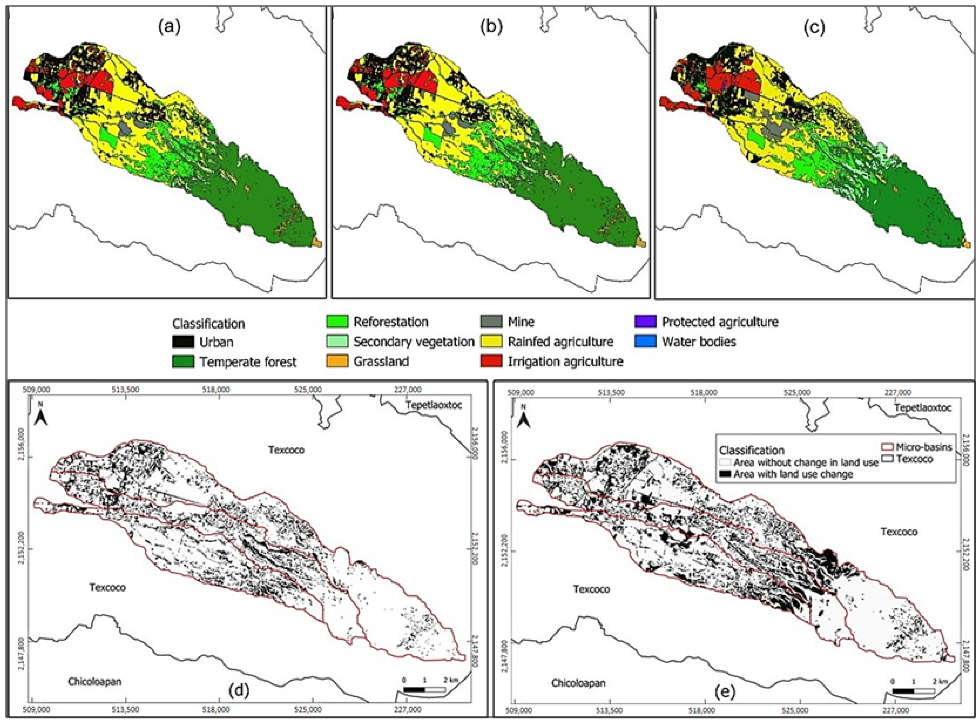
3.1. Changes in Land Use

It is extremely important to know the historical and current trends of the spatiotemporal variability of surface cover and changes [60]. Changes can modify the hydrological ecosystem balance. Figure 3 shows the results of the supervised classification for the years 1995, 2008, and 2021. In the 1995–2008 period, land use changed to 1246 ha, which represents 16% of the total area, as shown in Figure 3d. For the period 2008–2021 (Figure 3e), the change in land use affected 1906 ha or 24% of the total area. Between 1995 and 2008, the loss of temperate forest was 57.6 ha, but the loss in the period 2008–2021 was 323.9 ha. (Table 3). A decrease of 16.3% (in both periods) was mainly because of the affectation of two forest fires that occurred in 2012 and 2017 [61,62].

The changes in land use as a consequence of forest fires coincided with León [63]. High-severity forest fires have the capacity to disturb hydrological processes in forested watersheds, such as interception, infiltration, storage, and evapotranspiration [64,65]. The effects can be an increase in surface runoff, soil erosion, and sediment deposition [66,67,68]. Changes in the frequency and intensity of forest fires induced by climate change, outbreaks of insects and pathogens, and extreme phenomena, such as strong winds, may be more important than the direct impact of higher temperatures and elevated CO₂ [19].

As a result of forest degradation due to fires, secondary vegetation growth was 301.7 ha between 1995 and 2021 (

Table 4. Land use and vegetation (ha) in years 1995, 2008 and 2021; changes between 1995–2008 and 2008–2021.

Land Use Class	1995	%	2008	%	2021	%	1995–2008	2008–2021	Total Change	Change ha/Year
Temperate forest	2403.0	31.0	2345.4	30.3	2021.4	26.1	−57.6	−323.9	−381.6	−14.7
Reforestation	968.3	12.5	1104.6	14.3	1145.6	14.8	136.4	41.0	177.4	6.8
Secondary vegetation	137.0	1.8	300.7	3.9	438.7	5.7	163.7	138.0	301.7	11.6
Pasture	74.0	1.0	102.6	1.3	52.2	0.7	28.6	−50.3	−21.8	−0.8
Mine	147.8	1.9	124.2	1.6	212.2	2.7	−23.6	88.0	64.4	2.5
Rainfed agriculture	2530.0	32.7	2399.8	31.0	2294.8	29.6	−130.3	−105.0	−235.3	−9.0
Irrigated agriculture	664.4	8.6	483.6	6.2	540.3	7.0	−180.8	56.8	−124.1	−4.8
Protected agriculture	20.0	0.3	32.2	0.4	80.8	1.0	12.2	48.6	60.8	2.3
Urban	791.7	10.2	844.3	10.9	949.9	12.3	52.6	105.6	158.2	6.1
Water	4.3	0.1	3.2	0.0	4.6	0.1	−1.1	1.4	0.3	0.0

) since it was able to sprout quickly after a fire. This type of vegetation could thrive for a long time without succession being able to displace it [69]. The frequency of forest fires in Mexico has resulted in forest areas where secondary vegetation predominates [70].

However, there was a positive response in terms of restoring degraded land, with 184.2 ha of reforestation, which would greatly favor infiltration levels since by reducing surface runoff, the infiltration capacity of rain increases within the mineral soil [71,72].

Table 5. Land use changes (has) matrix between 1995–2008 and in the period 2008–2021.

	Land Use Classes	TF 1	R 2	SV 3	G 4	M 5	RA 6	IA 7	PA 8	U 9	W 10
		2008
1995	Secondary vegetation	34.7	4.3	-	0.9	-	-	2.7	-	-	-
	Reforestation	18.2	-	100.2	0.1	5.4	49.3	8.9	0.4	35.0	-
	Pasture	3.5	-	1.2	0.0	-	-	-	-	-	-
	Temperate forest	-	32.6	49.3	31.7	-	2.7	-	0.8	0.4	-
		2021
2008	Pasture	68.9	0.1	0.5	-	-	0.2	-	-	-	-
	Secondary vegetation	26.6	106.2	-	0.9	-	42.2	0.2	0.6	0.6	0.1
	Reforestation	14.4	-	31.9	0.1	8.2	197.1	53.8	3.4	42.6	0.2
	Temperate forest	-	131.5	280.9	18.3	-	4.1	-	-	-	-

¹ temperate forest, ² reforestation, ³ secondary vegetation, ⁴ grassland, ⁵ mine, ⁶ rainfed agriculture, ⁷ irrigated agriculture, ⁸ protected agriculture, ⁹ urban, ¹⁰ water bodies.

shows changes in land use. In the period 1995–2008, 32.6 and 49.3 ha of the temperate forest changed to reforestation and secondary vegetation, respectively. Reforestation areas changed mainly to secondary vegetation (100.2 ha) and rainfed agriculture (49.3 ha). For the period 2008–2021, the temperate forest changed to secondary vegetation (280.9 ha), and 131.5 ha changed to reforestation areas.

3.2. Future Scenarios (Land Use)

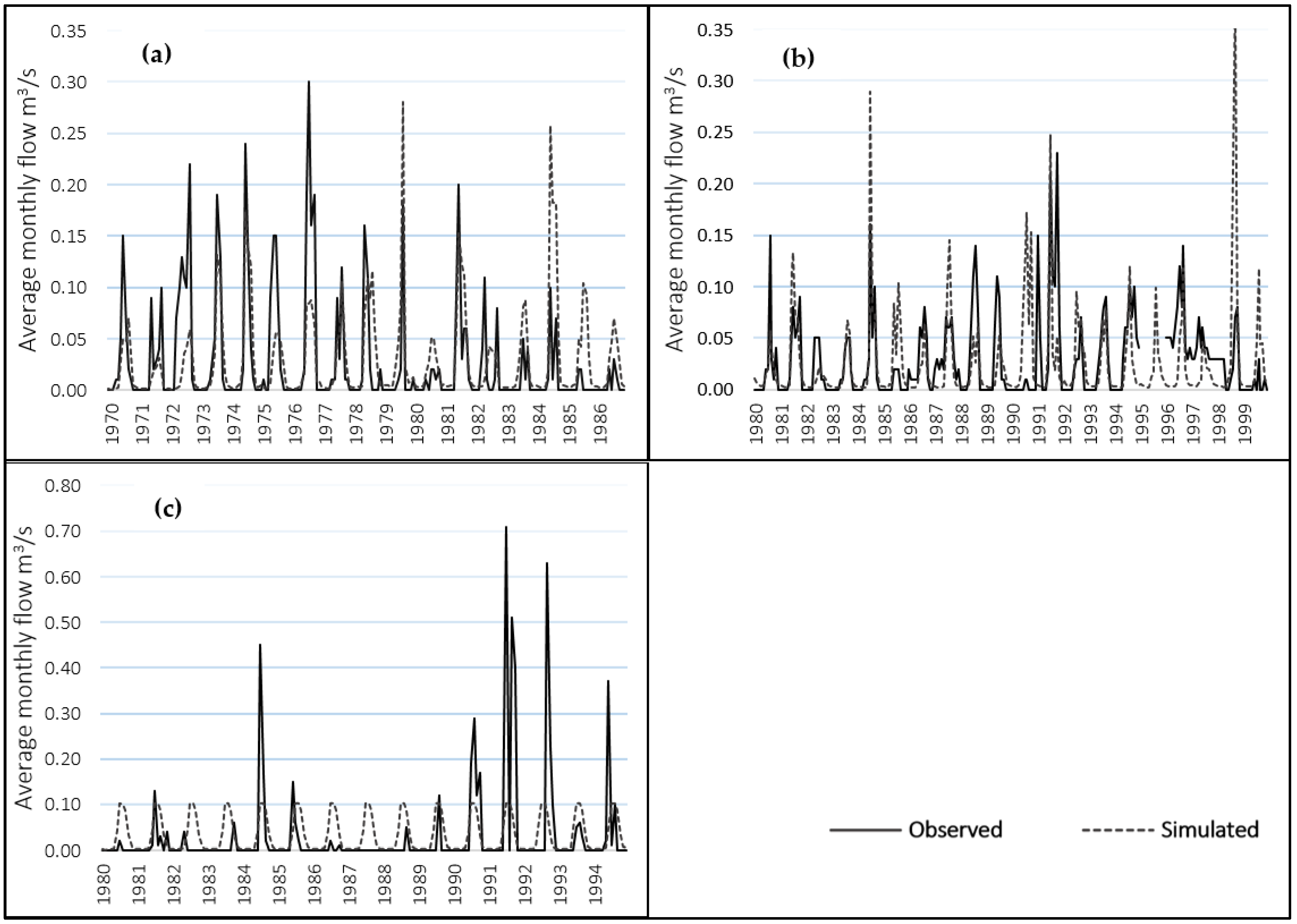
Aspects of vegetation cover change due to future trends can be considered in the land use scenarios. For example, they can consider a decrease or an increase in forest area or a change in the type of crops caused by economic trends. All of the scenarios should be studied so that when the scenario is implemented, it is clear what variables and functions will be taken into account when the scenario is defined [33]. The land cover areas used to design and project the scenarios are shown in

Table 6. Area (%) of reference years and current and future scenarios.

Land Use Class	Area (%)
	1995	2008	Current	Positive Scenario	Negative Scenario
Temperate forest	31.0	30.3	26.0	48.5	13.6
Reforestation	12.5	14.3	14.9	9.6	2.4
Secondary vegetation	1.8	3.9	5.7	0.3	4.9
Pasture	1.0	1.3	0.7	0	2.8
Mine	1.9	1.6	2.7	2.8	3.6
Agriculture (rainfed)	32.6	31.0	29.6	18.2	48.7
Agriculture (irrigated)	8.6	6.3	6.9	3.6	5.6
Agriculture (protected)	0.3	0.4	1.1	2.6	2.1
Urban	10.2	10.9	12.2	14.3	16.3
Water	0.1	0.0	0.1	0.1	0.1

.

3.3. Calibration

Calibration is a step to improve a model for a given set of local circumstances [53]. Calibration reduces the uncertainty of the prediction and can be considered parameter estimation or parameter optimization [73].

Figure 4a shows the comparison of observed and model-simulated monthly streamflow data in the Texcoco River. The model prediction of the hydrological response of the watershed was very good according to estimators (NSE = 0.98, R2 = 0.93, RSR = 0.15, and PBIAS = 5.3). It was also observed that the model was not able to simulate the peak flow rates and that the simulation was closer to the base flow rates. This performance of the model was different from the results of other studies [74], which described that WEAP better simulated the peak runoff of the base flows with data for the Conchos River basin in Mexico.

In the San Bernardino micro-watershed, the goodness-of-fit indicated that it was very good (NSE = 0.84, R2 = 0.76, and RSR = 0.38) and good (PBIAS = −13.5). The simulated flow showed repetitive behavior because the software accepts the results to be performed even if there are no rainfall records in the period. This was possible because the software allows the model to run with a full degree of accuracy when the data are available, or it can calculate it when the data are not available [75]. It was observed that when precipitation data were inputted with values estimated using isohyets, the model failed to reproduce the variation in peak flows, and the simulation was closer to the variation in base flows.

In Chapingo River, the goodness-of-fit indicated that the ability of the model to predict the hydrological response was very good (NSE = 0.93, R2 = 0.81, and RSR = 0.26). The simulation has overestimated the flow rate according to the PBIAS = −13.1 since, in most years, the peak flows were above the observed values. However, this percentage is considered good, and it was observed that the modeled curves (Figure 4b) of the base flows were closer to the records.

Goodness-of-fit. The ranges of calibration values were classified as very good, which indicated that the model properly simulated the hydrological responses of the three micro-watersheds [76]. Different studies have proved the capacity of WEAP to replicate hydrological processes in different parts of the world [77,78,79,80]. However, according to the sensitivity analysis, the validation presented values lower than those of the calibration period; however, it can be considered that the model maintained a satisfactory, good, and very good general performance based on the classification of the ranges of the estimators in the three microbasins. The difference between the ranges of the estimators of the calibration and validation period may be due to the fact that the conditions in the validation period were significantly different due to the increase in wastewater in the canals caused by the changes in land use that occurred in the study area.

3.4. Hydrological Balance

Estimating a basin’s water resources requires an understanding of the cycle in its various stages: the water inputs (precipitation or mist) is distributed between the runoff, infiltration, and evapotranspiration process [81]. The analysis includes the inflow variables (precipitation and water stored the preceding year) and the outflow (evapotranspiration, water storage in the soil, base flow, interflow, and surface runoff) of the hydrological balance. To determine how the hydrologic resource is distributed in the micro-watersheds of the study area, streamflow was used as an indicator. The results were compared with current information (2021) and the change (evolution in %) estimated in the projected scenarios by 2081–2100 (

Table 7. Hydrological balance (inflow and outflow) for three watersheds studied.

Scenario		Current	Negative			Positive
			CNRM	HADGEM	MPI	CNRM	HADGEM	MPI
Units		(mm/Year)	Evolution (%)
Texcoco River
Inflows	Precipitation	652.5	42.7	32.0	20.0	42.7	32.0	20.0
	Water stored *	130.7	23.8	9.5	3.9	43.1	23.8	17.5
Outflows	Evapotranspiration	533.7	32.7	30.7	19.1	41.7	37.3	24.9
	Water storage in the soil	199.8	29.6	13.4	7.1	46.7	24.8	17.7
	Base flow	4.1	−70.1	−74.3	−75.8	−67.1	−72.8	−74.6
	Inter flow	2.7	146.4	115.8	100.0	116.3	89.0	75.1
	Surface runoff	25.9	355.6	184.2	142.4	137.7	32.6	12.0
Chapingo River
Inflows	Precipitation	652.5	42.7	32.0	20.0	42.7	32.0	20.0
	Water stored *	108.5	−22.5	−25.5	−34.9	33.4	19.7	8.8
Outflows	Evapotranspiration	534.7	23.9	23.7	13.5	37.7	34.3	22.6
	Water storage in the soil	153.3	1.8	6.1	−15.0	46.5	27.9	17.3
	Base flow	4.2	−80.9	−81.5	−81.7	−80.3	−81.2	−81.5
	Inter flow	12.3	86.8	68.2	59.8	97.7	74.6	65.1
	Surface runoff	40.0	332.1	187.8	140.6	125.1	36.9	12.6
San Bernardino River
Inflows	Precipitation	652.5	42.7	32.0	20.0	42.7	32.0	20.0
	Water stored *	108.5	−6.4	−8.7	−20.6	106.3	82.3	67.5
Outflows	Evapotranspiration	534.7	17.7	18.3	8.6	34.3	30.9	19.5
	Water storage in the soil	153.3	21.1	13.0	2.5	103.7	76.2	62.7
	Base flow	4.2	−35.5	−41.2	−43.5	−29.8	−39.6	−42.6
	Inter flow	12.3	77.5	59.2	51.2	84.5	57.9	48.5
	Surface runoff	40.0	326.1	190.8	145.1	110.1	35.2	13.2

* Refers to water stored in the soil from the previous rainy season.

). The WEAP model assumes that land use does not change; however, it was possible to include the variable only by entering the projected values of land use change.

3.4.1. Projections of Future Hydrological Conditions

The simulations of the hydrological balance under the conditions of the positive scenario of land use change mainly implied an increase in the cover of the temperate forest (85.9%). The increase assumes that there will be no forest fires for the next 60 years, a situation that would allow for significant ecosystem restoration through both reforestation and natural regeneration. Similarly, a reduction in agricultural rain-fed use (−38.7%) near or within the preferred forest area was considered.

The results show that under the climatic conditions, mainly due to the influence of the precipitation regimes proposed by the GCMs, and despite the recovery of the ecosystem according to the positive scenario, an increase in surface runoff in the three microbasins is expected as follows: CNRM-CM6-1 model: Chapingo River (125.1%), Texcoco River (137.7%) and San Bernardino River (110.1%); HadGEM3-GC31-LL: Chapingo River (36.9%), Texcoco River (32.6) and San Bernardino River (35.2%); and MPI-ESM1-2-LR, Chapingo River (12%), Texcoco River (12.6%), and San Bernardino River (13.2%). These increases are indicators that despite the implementation of actions (reforestation, stimulation of natural regeneration, commercial plantations, control of fires, pests, and diseases) that mitigate the effects of climate change, it will be impossible to completely reverse the changes in the balance of the hydrological conditions, mainly due to the increase in precipitation and temperature values. However, a considerable decrease in surface runoff was observed: −46.2% (CNRM), −68.6% (HadGEM3), and −83.8% (MPI) in the entire study area compared to the scenario with negative land use change. With the increase in forest cover, there would be a smaller speed of runoff [72,82].

It was also observed that in the inflows by 2081–2100, there would be an average increase in the three microbasins of the water stored in the soil the previous year: 60.9% (CNRM), 41.9% (HadGEM3) and 31.3% (MPI), which for all the study area represents 53.7% more than that in the percentages of the scenarios under the conditions of the negative scenario of land use change. This input will increase water infiltration and recharge of aquifers [83]. An average increase in evapotranspiration of 37.9% (CNRM), 34.2% (HadGEM3), and 22.3% (MPI) would also be expected to be directly related to the increase in temperature and forest cover [84].

The hydrological balances under the conditions of the negative scenario of land use change were simulated with a decrease of 50.1% of forest cover due to the persistence of high-severity forest fires; additionally, these fires would cause a decrease of 81.7% of reforestation and would not allow the establishment of the natural regeneration of the forest. Therefore, in degraded areas, there would be a significant advance of rainfed agriculture (64.2%), preferably forest. The model indicates that surface runoff would increase under these conditions [60,63] in the three micro-watersheds: Chapingo River (332.1%, 187.8%, and 140.6%), Texcoco River (355.6%, 184.2%, and 142.4) and San Bernardino River (326.1%, 190.8% and 140.1%) according to the CNRM, HadGEM3, and MPI, respectively. Water stored in the soil decreased by −22.5% compared to the previous year (CNRM), −25.5% (HadGEM3), and −34.9% (MPI) for the Chapingo River would also be expected, and −6.4% (CNRM), −8.7% (HadGEM3) and −20.6% (MPI) for the San Bernardino River. The ability of the soil to store and control the flow of water depends largely on its penetration rate and depth, but disturbances such as changes in land use and fire are capable of altering the rate of these soil capacities [85]. These alterations occur because the soil is exposed to water erosion, compaction [86], and alterations in structure (disappearance of organic matter and microfauna, lower field capacity, and higher apparent density) [85]. The modification of these flows suggests that the availability of water that provides the hydrological ecosystem service will be compromised in the study area [87]. However, in the Texcoco River basin, the three models indicate increases of 23.8%, 9.5%, and 3.9%, respectively, in this inflow. This result may be related to the increase in the estimation of precipitation by the GCMs.

Although actual evapotranspiration is significantly related to the proportion of forest cover [88], despite the decrease in the forest according to the conditions of the negative scenario, the three models indicate an average increase in evapotranspiration in the three micro-watersheds: 24.8%, 24.2%, and 13.7%, respectively. This result could be related to the increase in precipitation and temperature values by the GCMs and may also be related to the modification of the hydrological balance [63,89].

3.4.2. Hydrological Environmental Service

Distributions of inflows and outflows of the hydrological balance by watershed as a percentage of the evolution (Ev%) of the change in the proposed scenarios are shown in Table 7. The evolution was estimated based on the current flows of the study area [27]. The results indicated that under the conditions of the positive scenario, together with the increase in the precipitation values estimated by the GCMs, there would be an increase in the water kept in the soil the preceding year: by 138.3% according to the CNRM model, by 102.7% according to the HadGEM3 model and by 91.5% according to the MPI model. These percentages mean that in the parts of the micro-watersheds where temperate forest cover predominates, 77.4% (CNRM), 61% (HadGEM3), and 60% (MPI) would be stored more than in the current scenario at the micro-watershed level. Soil cover significantly influences the distribution of soil moisture [90,91].

However, although it is estimated that there would be much more moisture in the soil that would lead to the infiltration and recharge of the aquifers, the simulations indicate that there would be a decrease in the base flow, even under the conditions of the positive scenario: −52.5% (CNRM), −61.3% (HadGEM3) and −62.5% (MPI). This decrease could be related to the increase in evapotranspiration: 50.8% (CNRM), 43.3% (HadGEM3), and 30.2% (MPI). Climate change will accelerate the hydrological cycle with a tendency to increase temperature [10]. An increase in air temperature leads to higher rates of evapotranspiration [14]. These results coincide with the research conducted by Bazzi et al. [10], who reported that the greatest increase in evapotranspiration rates will occur in the period 2071–2100. Given that evapotranspiration is key in the hydrological balance, a disturbance to this flow can change the distribution between the dominant water flows, such as infiltration and surface runoff [65]. Some simulation studies suggest that increased precipitation, together with warmer temperatures in the summer, cause severe reductions in base flows [92,93]. However, at the local scale, high summer temperatures and increased evapotranspiration rates could lead to an increase in convective precipitation, which would compensate for the reductions in base flow [94]. The decrease in base flow may be related to the increase in forest cover, mainly due to the establishment of reforestation that has positive responses to the increase in soil moisture [95]. Regarding the evolution of the change that the surface runoff would present, under a negative scenario, it is expected that climatic changes will considerably increase the surface runoff in these parts of the micro-watersheds: 275% (CNRM), 127.7% (HadGEM3) and 133.8% (MPI). This result represents that in this part of the micro-watersheds, 81.6% (CNRM), 68.1% (HadGEM3), and 93.8% (MPI) of the total runoff from the micro-watersheds are generated. Removal of vegetative cover and soil organic matter leads to changes in hydrological processes by reducing interception of precipitation and altering soil structure (compaction and erosion), which results in an increase in the amount and speed of surface runoff [23,24,96]. The decrease in forest cover as a consequence of forest fires influences the increase in surface runoff, erosion, and the increase in sediments to the channels [66,67,68].

However, under the conditions of the positive scenario of land use change, the results contrary to the data presented at the microbasin level are observed, and it is emphasized that the variations in climate change would be contained at least in the parts of the microbasins where forest cover is present. The simulations indicate that there would be an average decrease in surface runoff of −69.9% (CNRM), −86.5% (HadGEM3), and −89.3% (MPI). This represents a decrease of −194.2% (CNRM), −121.1% (HadGEM3), and −101.9% (MPI) with respect to the data presented at the microbasin level for the same scenarios. The decrease in surface runoff is related to the interception of rain by the canopy [97]. The canopy is essential for soil conservation due to its role in decreasing the erosive impact of precipitation [98]. Another factor that reduces surface runoff is the incorporation of organic matter [99], promoting water infiltration to the root zone.

In this context, the results obtained highlight that forest cover itself plays a fundamental role in mitigating the impacts of climate change [100,101]. The forests of Mexico are the central axis of the institutional design that the country must face its commitments on climate change since it is estimated that 30% of the reduction of CO₂ emissions can be achieved if deforestation is avoided and if forest degradation and recovery of forest areas are achieved [102]. Forests are a viable way to combat the effects of climate change because they are efficient at sequestering and storing atmospheric carbon [20]. Therefore, the hydrological functions are more efficient in watersheds with forest cover [103].

4. Conclusions

A major cause of the decline in temperate forest cover in the study area is the frequency of forest fires; between 1995 and 2021, forest area declined by 16%. The climatic changes and land use changes could be integrated into WEAP software to measure the trajectories and hydrological responses of the micro-watersheds. The WEAP model was calibrated and validated to predict the hydrological response in the three micro-watersheds in an acceptable manner.

According to the models, the climatic changes presented by the GCMs under the most drastic scenario conditions, SSP5-8.5, will significantly modify the balance and distribution of the hydrological balance flows at the microbasin level, mainly due to the increase in the values of precipitation and temperature. Even under the conditions of the positive scenario of land use change that would imply the application of actions (reforestation, stimulation of natural regeneration, commercial plantations, fire control) that would mitigate the effects of climate change, it would be impossible to completely reverse the changes in hydrological balance. The imbalance would be reflected mainly in the amount and distribution of surface runoff, evapotranspiration, soil moisture, and base flow.

However, in the upper parts of the microbasins where temperate forest predominates, the climatic variations of the SSP5-8.5 scenarios could be contained under the conditions of the positive scenario of land use change. The simulations of the three GCMs indicated that there would be an average decrease in surface runoff and an increase in soil moisture compared with the current values and with the negative scenarios of land use change. This means that the conservation, management, and increase in the cover of the temperate forest can mitigate part of the impacts caused by climate change. However, under these conditions in the surfaces where the temperate forest predominates, there would also be modifications of the hydrological balance, mainly the increase in evapotranspiration (caused by the increase in temperature and seasonal precipitation), which would influence significant decreases in the low flow and interflow. The alteration of these last two flows will decrease the water available in the soil.

It is expected that the decrease in temperate forest cover caused by forest fires will intensify due to extreme climate changes (temperature and wind), conditions that will modify the natural regime of fire. This will cause significant alterations in the hydrological balance, mainly by reducing the rain interception of the canopy, increasing surface runoff velocity and flow, and altering soil structure and composition; therefore, there would be a reduction in the infiltration and recharge rates of aquifers. Therefore, the availability of hydrological and environmental services will be compromised in the aquifer to which the study area belongs. It will not be possible to meet the demand for groundwater, especially for public use in the urban areas of the region.

References

1. CONAGUA (Comisión Nacional de Agua). Atlas Del Agua En México 2015, 1st ed.; CONAGUA: Ciudad de México, México, 2015; ISBN 9788578110796. [Google Scholar]
2. Brauman, K.A. Hydrologic Ecosystem Services: Linking Ecohydrologic Processes to Human Well-Being in Water Research and Watershed Management. Wiley Interdiscip. Rev. Water 2015, 2, 345–358. [Google Scholar] [CrossRef]
3. Manson, R.H. Los Servicios Hidrológicos y La Conservación de Los Bosques de México. Madera Bosques 2016, 10, 3–20. [Google Scholar] [CrossRef]
4. Zilberman, D.; Lipper, L.; McCarthy, N. Putting Payments for Environmental Services in the Context of Economic Development. Paym. Environ. Serv. Agric. Landsc. 2009, 31, 9–33. [Google Scholar] [CrossRef]
5. Isik, S.; Kalin, L.; Schoonover, J.E.; Srivastava, P.; Graeme Lockaby, B. Modeling Effects of Changing Land Use/Cover on Daily Streamflow: An Artificial Neural Network and Curve Number Based Hybrid Approach. J. Hydrol. 2013, 485, 103–112. [Google Scholar] [CrossRef]
6. Brauman, K.A.; Daily, G.C.; Duarte, T.K.E.; Mooney, H.A. The Nature and Value of Ecosystem Services: An Overview Highlighting Hydrologic Services. Annu. Rev. Environ. Resour. 2007, 32, 67–98. [Google Scholar] [CrossRef]
7. Balvanera, P.; Cotler, H.; Aburto, O.; Aguilar, A.; Aguilera, M.; Aluja, M.; Andrade, A.; Arroyo, I.; Ashworth, L. Estado y tendencias de los servicios ecosistémicos. In Capital Natural de México, Vol. II: Estado de Conservación y Tendencias de Cambio; CONABIO: Ciudad de Mexico, Mexico, 2009; pp. 185–245. [Google Scholar]
8. Vitousek, P.M. Beyond Global Warming: Ecology and Global Change. Ecology 1994, 75, 1861–1876. [Google Scholar] [CrossRef]
9. Camarero, J.J.; Lloret, F.; Corcuera, L.; Peñuelas, J.; Gil-pelegrín, E. CAPÍTULO 14 Cambio global y decaimiento del bosque. In Ecologia del Bosque Mediterraneo en un Mundo Cambiante; Egraf, S.A., Ed.; Ministerio de Medio Ambiente: Madrid, Spain, 2004; pp. 397–423. ISBN 8480145528. [Google Scholar]
10. Bazzi, H.; Ebrahimi, H.; Aminnejad, B. A Comprehensive Statistical Analysis of Evaporation Rates under Climate Change in Southern Iran Using WEAP (Case Study: Chahnimeh Reservoirs of Sistan Plain). Ain. Shams. Eng. J. 2021, 12, 1339–1352. [Google Scholar] [CrossRef]
11. Ougougdal, H.A.; Khebiza, M.Y.; Messouli, M.; Lachir, A. Assessment of Futurewater Demand and Supply under IPCC Climate Change and Socio-Economic Scenarios, Using a Combination of Models in Ourika Watershed, High Atlas, Morocco. Water 2020, 12, 1751. [Google Scholar] [CrossRef]
12. Mena, D.; Solera, A.; Restrepo, L.; Pimiento, M.; Cañón, M.; Duarte, F. An Analysis of Unmet Water Demand under Climate Change Scenarios in the Gualí River Basin, Colombia, through the Implementation of Hydro-Bid and Weap Hydrological Modeling Tools. J. Water Clim. Chang. 2021, 12, 185–200. [Google Scholar] [CrossRef]
13. Pham, B.A.O.Q.; Yu, P.; Yang, T.; Kuo, C.; Tseng, H. Assessment of Climate Change Impacts on Hydrological Processes and Water Resources By Water Evaluation and Planning (Weap) Model: Case Study in Thac Mo Catchment, Vietnam. In Proceedings of the 37th IAHR World Congress, Kuala Lumpur, Malaysia, 13–18 August 2017; Volume 6865, pp. 4312–4321. [Google Scholar]
14. Wang, K.; Dickinson, R.E.; Liang, S. Global Atmospheric Evaporative Demand over Land from 1973 to 2008. J. Clim. 2012, 25, 8353–8361. [Google Scholar] [CrossRef]
15. López, G.T.G.; Manzano, M.G.; Ramírez, A.I. Disponibilidad Hídrica Bajo Escenarios de Cambio Climático En El Valle de Galeana, Nuevo León, México. Tecnol. Cienc. Agua. 2017, 8, 105–114. [Google Scholar] [CrossRef]
16. Rochdane, S.; Reichert, B.; Messouli, M.; Babqiqi, A.; Khebiza, M.Y. Climate Change Impacts on Water Supply and Demand in Rheraya Watershed (Morocco), with Potential Adaptation Strategies. Water 2012, 4, 28–44. [Google Scholar] [CrossRef] [Green Version]
17. Kerns, B.K.; Powell, D.C.; Mellmann-Brown, S.; Carnwath, G.; Kim, J.B. Effects of Projected Climate Change on Vegetation in the Blue Mountains Ecoregion, USA. Clim. Serv. 2018, 10, 33–43. [Google Scholar] [CrossRef]
18. Gutiérrez, E.; Trejo, I. Efecto Del Cambio Climático En La Distribución Potencial de Cinco Especies Arbóreas de Bosque Templado En México. Rev. Mex. Biodivers. 2014, 85, 179–188. [Google Scholar] [CrossRef] [Green Version]
19. Kirilenko, A.P.; Sedjo, R.A. Climate Change Impacts on Forestry. Proc. Natl. Acad. Sci. USA 2007, 104, 19697–19702. [Google Scholar] [CrossRef] [PubMed] [Green Version]
20. Rijal, S.; Sinutok, S.; Techato, K.; Gentle, P.; Khanal, U.; Gyawali, S. Contribution of Community-Managed Sal-Based Forest in Climate Change Adaptation and Mitigation: A Case from Nepal. Forests 2022, 13, 262. [Google Scholar] [CrossRef]
21. Clark, J.S.; Bell, D.M.; Hersh, M.H.; Nichols, L. Climate Change Vulnerability of Forest Biodiversity: Climate and Competition Tracking of Demographic Rates. Glob. Chang. Biol. 2011, 17, 1834–1849. [Google Scholar] [CrossRef]
22. Seidl, R.; Thom, D.; Kautz, M.; Martin-Benito, D.; Peltoniemi, M.; Vacchiano, G.; Wild, J.; Ascoli, D.; Petr, M.; Honkaniemi, J.; et al. Forest Disturbances under Climate Change. Nat. Clim. Chang. 2017, 7, 395–402. [Google Scholar] [CrossRef] [Green Version]
23. Aboelnour, M.; Gitau, M.W.; Engel, B.A. A Comparison of Streamflow and Baseflow Responses to Land-Use Change and the Variation in Climate Parameters Using SWAT. Water 2020, 12, 191. [Google Scholar] [CrossRef] [Green Version]
24. Khoshnoodmotlagh, S.; Verrelst, J.; Daneshi, A.; Mirzaei, M.; Azadi, H.; Haghighi, M.; Hatamimanesh, M.; Marofi, S. Transboundary Basins Need More Attention: Anthropogenic Impacts on Land Cover Changes in Aras River Basin, Monitoring and Prediction. Remote Sens. 2020, 12, 3329. [Google Scholar] [CrossRef]
25. CONAFOR (Comisión Nacional Forestal). Programas y Acciones En Reforestación, Conservación y Restauración de Suelos, Incendios Forestales y Sanidad Forestal de Ecosistemas Forestales; Comisión Nacional Forestal (CONAFOR): Zapopan, Jalisco, 2010. [Google Scholar]
26. Kepner, W.G.; Ramsey, M.M.; Brown, E.S.; Jarchow, M.E.; Dickinson, K.J.M.; Mark, A.F.; Ramsey, E.M.S.; Brown, M.E.; Jarchow, K.J.M.; Dickinson, A.F. Hydrologic Futures: Using Scenario Analysis to Evaluate Impacts of Forecasted Land Use Change on Hydrologic Services. Ecosphere 2012, 3, 1–25. [Google Scholar] [CrossRef]
27. Ruíz-García, V.H.; Borja de la Rosa, M.A.; Gómez-Díaz, J.D.; Asensio-Grima, C.; Matías-Ramos, M.; Monterroso-Rivas, A.I. Forest Fires, Land Use Changes and Their Impact on Hydrological Balance in Temperate Forests of Central Mexico. Water 2022, 14, 383. [Google Scholar] [CrossRef]
28. Rubio Camacho, E.A.; González Tagle, M.A.; Benavides Solorio, J.D.D.; Chávez Durán, Á.A.; Xelhuantzi Carmona, J. Relación Entre Necromasa, Composición de Especies Leñosas y Posibles Implicaciones Del Cambio Climático En Bosques Templados. Rev. Mex. Cienc. Agrícolas 2017, 13, 2601–2614. [Google Scholar] [CrossRef] [Green Version]
29. Vargas, C.R.d.C.; Sanchez, T.G.; Rolón, A.J.C.; Pichardo, R.R.; Tobías, J.R.; Treviño, T.J. Disponibilidad de los Recursos Hídricos ante Escenarios de Cambio Climático en una Cuenca Costera de Tamaulipas, México. Investig. Actuales En Medioambiente 2015, 1, 86–100. [Google Scholar]
30. Escoto Castillo, A.; Sánchez Peña, L.; Gachuz Delgado, S. Trayectorias Socioeconómicas Compartidas (SSP): Nuevas Maneras de Comprender El Cambio Climático y Social. Estud. Demogr. Urbanos. Col. Mex. 2017, 32, 669–693. [Google Scholar] [CrossRef] [Green Version]
31. Esquivel-Arriaga, G.; Nevarez-Favela, M.M.; Velásquez-Valle, M.A.; Sánchez-Cohen, I.; Bueno-Hurtado, P. Hydrological Modeling of a Basin in Mexico’s Arid Northern Region and Its Response to Environmental Changes. Ing. Agrícola Biosist. 2017, 9, 3–17. [Google Scholar] [CrossRef] [Green Version]
32. SEI (Stockholm Environmental Institute). Water Evaluation And Planning System Tutorial; Stockholm Environmental Institute: Stockholm, Sweden, 2017. [Google Scholar]
33. Centro de Cambio Global-Universidad Católica de Chile; Stockholm Environment Institute. Guía Metodológica-Modelación Hidrológica y de Recursos Hídricos Con El Modelo WEAP; Stockholm Environment Institute: Stockholm, Sweden, 2009. [Google Scholar]
34. Amato, C.C.; Daene, P.E.; Mckinney, C.; Ingol-Blanco, E.; Teasley, R.L. CRWR Online Report 06-12 WEAP Hydrology Model Applied: The Rio Conchos Basin; The University of Texas: Austin, TX, USA, 2006. [Google Scholar]
35. Ahmadaali, J.; Barani, G.-A.; Qaderi, K.; Hessari, B. Analysis of the Effects of Water Management Strategies and Climate Change on the Environmental and Agricultural Sustainability of Urmia Lake Basin, Iran. Water 2018, 10, 160. [Google Scholar] [CrossRef] [Green Version]
36. Geler, R.T.; Toruño, P.J.; Marinero Orantes, E.A.; Gutiérrez Espinoza, E.I. Servicios Ambientales y Gestión de Los Recursos Hídricos Utilizando El Modelo WEAP: Casos de Estudio En Iberoamérica. Rev. Iberoam. Bioeconomía Cambio Climático 2015, 1, 72–87. [Google Scholar] [CrossRef] [Green Version]
37. Yates, D.; Sieber, J.; Purkey, D.; Huber-Lee, A. WEAP21—A Demand-, Priority-, and Preference-Driven Water Planning Model. Part 1: Model Characteristics. Water Int. 2005, 30, 487–500. [Google Scholar] [CrossRef]
38. Labrador, A.F.; Zúñiga, J.M.; Romero, J. Desarrollo de Un Modelo Para La Planificación Integral Del Recurso Hídrico En La Cuenca Hidrográfica Del Río Aipe, Huila, Colombia Development of a Model for Integral Planning of Water Resources in Aipe Catchment, Huila, Colombia. Rev. Ing. Región 2016, 15, 23–35. [Google Scholar] [CrossRef] [Green Version]
39. Flores, L.F.; Galaitsi, S.; Escobar, M.; Purkey, D. Modeling of Andean Páramo Ecosystems’ Hydrological Response to Environmental Change. Water 2016, 8, 94. [Google Scholar] [CrossRef]
40. IPCC (Intergovernmental Panel on Climate Change). Summary for policymakers. In Climate Change 2021: The Physical Science Basis; Contribution of Working Group I to the Sixth Assessment Report of the Intergovernmental Panel on Climate Change; Masson-Delmotte, V.P., Zhai, A.P., Connors, S., Péan, C., Berger, S., Caud, N., Chen, Y., Goldfarb, L., Gomis, M., Huang, M., et al., Eds.; Cambridge University Press: Cambridge, UK, 2021; pp. 3–32. ISBN 9781317602071. [Google Scholar]
41. SEMARNAT (Secretaría de Medio Ambiente). Acuerdo Por El Que Se Dan a Conocer Los Resultados del Estudio Técnico de Las Aguas Nacionales Subterráneas del Acuífero Texcoco, Clave 1507, En El Estado de México, Región Hidrológico-Administrativa XIII, Aguas del Valle de México; SEMARNAT: Ciudad de México, Mexico, 2019. [Google Scholar]
42. Garcia, E. Modificaciones al Sistema de Clasificación Climática de Köppe; UNAM, Ed.; Universidad Nacional Autónoma de México: Ciudad de México, México, 2004; ISBN 970-32-1010-4. [Google Scholar]
43. SMN (Servicio Metereológico Nacional). Información Climatológica Nacional. Available online: https://smn.conagua.gob.mx/es/climatologia/informacion-climatologica/informacion-estadistica-climatologica (accessed on 3 June 2022).
44. Gómez-Díaz, J.; Etchevers-Barra, J.; Monterroso-Rivas, A.; Gay-García, C.; Campo-Alves, J.; Martínez-Menes, M. Spatial Estimation of Mean Temperature and Precipitation in Areas of Scarce Meteorological Information. Atmósfera 2008, 21, 35–56. [Google Scholar]
45. Gómez-Díaz, J.; Monterroso-Rivas, A.I. Actualización de La Delimitación de Las Zonas Áridas, Semiáridas y Sub-Húmedas Secas de México a Escala Regional. Reporte Final de Proyecto de Investigación Fondo CONAFOR-CONACYT; Universidad Autonoma Chapingo: Texcoco, México, 2008. [Google Scholar]
46. Young, C.A.; Escobar-Arias, M.I.; Fernandes, M.; Joyce, B.; Kiparsky, M.; Mount, J.F.; Mehta, V.K.; Purkey, D.; Viers, J.H.; Yates, D. Modeling the Hydrology of Climate Change in California’s Sierra Nevada for Subwatershed Scale Adaptation. J. Am. Water Resour. Assoc. 2009, 45, 1409–1423. [Google Scholar] [CrossRef]
47. Monterroso-Rivas, A.I.; Gómez-Díaz, J.D. Impact of Climate Change on Potential Evapotranspiration and Growing Season in Mexico. Rev. TERRA Lat. 2021, 39, 1–19. [Google Scholar] [CrossRef]
48. Santos-Hernández, A.F.; Monterroso-Rivas, A.I.; Granados-Sánchez, D.; Villanueva-Morales, A.; Santacruz-Carrillo, M. Projections for Mexico’s Tropical Rainforests Considering Ecological Niche and Climate Change. Forests 2021, 12, 119. [Google Scholar] [CrossRef]
49. Ruiz-García, P.; Conde-Álvarez, C.; Gómez-Díaz, J.D.; Monterroso-Rivas, A.I. Projections of Local Knowledge-Based Adaptation Strategies of Mexican Coffee Farmers. Climate 2021, 9, 60. [Google Scholar] [CrossRef]
50. Congedo, L. Semi-Automatic Classification Plugin: A Python Tool for the Download and Processing of Remote Sensing Images in QGIS. J. Open Source Softw. 2021, 6, 3172. [Google Scholar] [CrossRef]
51. CONAGUA (Comisión Nacional del Agua). Banco Nacional de Datos de Aguas Superficiales (BANDAS). Available online: https://app.conagua.gob.mx/bandas/ (accessed on 3 June 2022).
52. Jantzen, T.; Klezendorf, B.; Middleton, J.; Smith, J. WEAP Hydrology Modeling Applied: The Upper Rio Florido Rive Basin; Center for Research in Water Resources: Ciudad de México, México, 2006. [Google Scholar]
53. Arnold, J.G.; Moriasi, D.N.; Gassman, P.W.; Abbaspour, K.C.; White, M.J. SWAT: Model Use, Calibration, and Validation. Trans. ASABE 2012, 55, 1549–1559. [Google Scholar] [CrossRef]
54. Gupta, H.V.; Sorooshian, S.; Hogue, T.S.; Boyle, D.P. Advances in automatic calibration of watershed models. In Calibration of Watershed Models; American Geophysical Union: Washington, DC, USA, 2011; pp. 9–28. [Google Scholar]
55. Lu, C.; Chiang, L.-C. Assessment of Sediment Transport Functions with the Modified SWAT-Twn Model for a Taiwanese Small Mountainous Watershed. Water 2019, 11, 1749. [Google Scholar] [CrossRef] [Green Version]
56. Nash, J.E.; Sutcliffe, J.V. River Flow Forecasting Through Conceptual Models—Part I—A Discussion of Principles. J. Hydrol. 1970, 10, 282–290. [Google Scholar] [CrossRef]
57. Vijai, H.; Sorooshian, S.; Yapo, P. Status of Automatic Calibration for Hydrologic Models: Comparison with Multilevel Expert Calibration. J. Hydrol. Eng. 1999, 4, 135–143. [Google Scholar]
58. Singh, J.; Knapp, H.; Demissie, M. Hydrologic Modeling of the Iroquois River Watershed Using HSPF and SWAT. J. Am. Water Resour. Assoc. 2005, 4030, 343–360. [Google Scholar] [CrossRef]
59. Zambrano-Bigiarini, M. HydroGOF: Goodness-of-Fit Functions for Comparison of Simulated and Observed Hydrological Time Series, R Package Version 0.4-0. 2020. [Google Scholar]
60. Martínez Sifuentes, A.R.; Villanueva Díaz, J.; Estrada Ávalos, J.; Vázquez Vázquez, C.; Orona Castillo, I. Pérdida de Suelo y Modificación de Escurrimientos Causados Por El Cambio de Uso de La Tierra En La Cuenca Del Río Conchos, Chihuahua. Nov. Sci. 2020, 12. [Google Scholar] [CrossRef]
61. Hernández, G.A.; Castorena, M.D.C.G.; Maravilla, S.M.B.; Cervantes, E.R.Á.; Castorena, E.V.G.; Solorio, C.A.O. Mineralogy in the Estimation of the Temperature of Forest Fire and Their Immediate Effects in Andosols, State of Mexico. Madera Bosques 2020, 26, 1–14. [Google Scholar] [CrossRef]
62. PROBOSQUE (Protectora de bosques del Estado de México). Estadisticas de Incendios Forestales En El Estado de México: Administrador de Base de Datos PostGIS. Available online: https://probosque.edomex.gob.mx/estadisticas (accessed on 20 September 2022).
63. León-Muñoz, J.; Aguayo, R.; Marcé, R.; Catalán, N.; Woelfl, S.; Nimptsch, J.; Arismendi, I.; Contreras, C.; Soto, D.; Miranda, A. Climate and Land Cover Trends Affecting Freshwater Inputs to a Fjord in Northwestern Patagonia. Front. Mar. Sci. 2021, 8, 628454. [Google Scholar] [CrossRef]
64. Ebel, B.A.; Moody, J.A. Synthesis of Soil-Hydraulic Properties and Infiltration Timescales in Wildfire-Affected Soils. Hydrol. Process. 2017, 31, 324–340. [Google Scholar] [CrossRef]
65. Poon, P.K.; Kinoshita, A.M. Spatial and Temporal Evapotranspiration Trends after Wildfire in Semi-Arid Landscapes. J. Hydrol. 2018, 559, 71–83. [Google Scholar] [CrossRef]
66. Kinoshita, A.M.; Chin, A.; Simon, G.L.; Briles, C.; Hogue, T.S.; O’Dowd, A.P.; Gerlak, A.K.; Albornoz, A.U. Wildfire, Water, and Society: Toward Integrative Research in the “Anthropocene”. Anthropocene 2016, 16, 16–27. [Google Scholar] [CrossRef] [Green Version]
67. Rengers, F.K.; McGuire, L.A.; Kean, J.W.; Staley, D.M.; Hobley, D.E.J. Water Resources Research. J. Am. Water Resour. Assoc. 1969, 5, 2-2. [Google Scholar] [CrossRef]
68. Robichaud, P.R.; Wagenbrenner, J.W.; Pierson, F.B.; Spaeth, K.E.; Ashmun, L.E.; Moffet, C.A. Infiltration and Interrill Erosion Rates after a Wildfire in Western Montana, USA. Catena 2016, 142, 77–88. [Google Scholar] [CrossRef] [Green Version]
69. Rzedowski, J. Vegetación de México; Primera, Ed.; Comisión Nacional para el Conocimiento y Uso de la Biodiversidad: Ciudad de México, México, 2006. [Google Scholar]
70. Miranda, F.; Hernández, X.E. Los Tipos de Vegetación de México y Su Clasificación. Bot. Sci. 2016, 28, 29–179. [Google Scholar] [CrossRef] [Green Version]
71. Laino-Guanes, R.; Suárez-Sánchez, J.; González-Espinosa, M.; Musálem-Castillejos, K.; Ramírez-Marcial, N.; Bello-Mendoza, R.; Jiménez, F. Modelación Del Balance Hídrico y El Movimiento de Nutrientes Utilizando WEAP: Limitaciones Para Modelar Los Efectos de La Restauración Forestal y El Cambio Climático En La Cuenca Alta Del Río Grijalva. Aqua-LAC 2017, 9, 46–58. [Google Scholar] [CrossRef]
72. Urrutia Hernández, I.; Rodríguez Alfaro, B.; González Menéndez, M.; Martínez Becerra, L.W.; Flores Garnica, J.G.; Alonso Torrens, Y. Impacto de Quemas Prescritas En La Estabilidad Del Escurrimiento Superficial En Un Bosque de Pino. Madera Bosques 2020, 26, 1–12. [Google Scholar] [CrossRef]
73. Droogers, P.; Immerzeel, W.W. Calibration Methodologies in Hydrological Modeling: State of the Art; The National User Support Programme 2001–2005; FutureWater-Science for Solutions: Wageningen, The Netherlands, 2006. [Google Scholar]
74. Ingol-Blanco, E.; McKinney, D.C. Development of a Hydrological Model for the Rio Conchos Basin. J. Hydrol. Eng. 2013, 18, 340–351. [Google Scholar] [CrossRef]
75. Kandera, M.; Výleta, R.; Liová, A.; Danáčová, Z.; Lovasová, Ľ. Testing of Water Evaluation and Planning (Weap) Model for Water Resources Management in the Hron River Basin. Acta Hydrol. Slovaca 2021, 22, 30–39. [Google Scholar] [CrossRef]
76. Moriasi, D.N.; Arnold, J.G.; Van Liew, M.W.; Bingner, R.L.; Harmel, R.D.; Veith, T.L. Model Evaluation Guidelines for Systematic Quantification of Accuracy in Watershed Simulations. Trans. ASABE 2007, 50, 885–900. [Google Scholar] [CrossRef]
77. Abera Abdi, D.; Ayenew, T. Evaluation of the WEAP Model in Simulating Subbasin Hydrology in the Central Rift Valley Basin, Ethiopia. Ecol. Process. 2021, 10, 41. [Google Scholar] [CrossRef]
78. Asghar, A.; Iqbal, J.; Amin, A.; Ribbe, L. Integrated Hydrological Modeling for Assessment of Water Demand and Supply under Socio-Economic and IPCC Climate Change Scenarios Using WEAP in Central Indus Basin. J. Water Supply Res. Technol.-AQUA 2019, 68, 136–148. [Google Scholar] [CrossRef] [Green Version]
79. Al-Mukhtar, M.M.; Mutar, G.S. Modelling of Future Water Use Scenarios Using WEAP Model: A Case Study in Baghdad City, Iraq. Eng. Technol. J. 2021, 39, 488–503. [Google Scholar] [CrossRef]
80. Nevárez-Favela, M.M.; Fernández-Reynoso, D.S.; Sánchez-Cohen, I.; Sánchez-Galindo, M.; Macedo-Cruz, A.; Palacios-Espinosa, C. Comparison between WEAP and SWAT Models in a Basin at Oaxaca, Mexico. Tecnol. Cienc. Agua. 2021, 12, 358–401. [Google Scholar] [CrossRef]
81. García-Coll, I.; Martínez, A.; Ramírez, A.; Niño, A.; Rivas, A.; Domínguez, L. La relación agua-bosque: Delimitación de zonas prioritarias para pago de servicios ambientales hidrológicos en la cuenca del río Gavilanes, Coatepec, Veracruz. In El Manejo Integral de Cuencas en México; Cotler, H., Ed.; Instituto Nacional de Ecología: Ciudad de México, Mexico, 2004; pp. 99–116. [Google Scholar]
82. Viramontes, D.; Descroix, L.; Bollery, A. Variables de Suelos Determinantes Del Escurrimiento y La Erosión En Un Sector de La Sierra Madre Occidental. Ing. Hidraul. Mex. 2006, 21, 73–83. [Google Scholar]
83. La Manna, L.; Rostagno, M.; Morales, D. Impacto Del Fuego Sobre El Comportamiento Hidrológico Del Suelo En Un Bosque de Ciprés. Patagon For. 2010, 16, 23–24. [Google Scholar]
84. Mab, P.; Kositsakulchai, E. Water Balance Analysis of Tonle Sap Lake Using Weap Model and Satellite-Derived Data from Google Earth Engine. Sci. Technol. Asia 2020, 25, 45–58. [Google Scholar] [CrossRef]
85. Poca, M.; Cingolani, A.M.; Gurvich, D.E.; Whitworth-Hulse, J.I.; Saur Palmieri, V. La Degradación de Los Bosques de Altura Del Centro de Argentina Reduce Su Capacidad de Almacenamiento de Agua. Ecol. Austral. 2018, 28, 235–248. [Google Scholar] [CrossRef] [Green Version]
86. Bruijnzeel, L.A. Hydrological Functions of Tropical Forests: Not Seeing the Soil for the Trees? Agric. Ecosyst. Environ. 2004, 104, 185–228. [Google Scholar] [CrossRef]
87. Nelson, E.; Mendoza, G.; Regetz, J.; Polasky, S.; Tallis, H.; Cameron, D.R.; Chan, K.M.A.; Daily, G.C.; Goldstein, J.; Kareiva, P.M.; et al. Modeling Multiple Ecosystem Services, Biodiversity Conservation, Commodity Production, and Tradeoffs at Landscape Scales. Front. Ecol. Environ. 2009, 7, 4–11. [Google Scholar] [CrossRef]
88. Tena, T.M.; Mwaanga, P.; Nguvulu, A. Impact of Land Use/Land Cover Change on Hydrological Components in Chongwe River Catchment. Sustainability 2019, 11, 6415. [Google Scholar] [CrossRef] [Green Version]
89. Fan, M.; Shibata, H.; Wang, Q. Optimal Conservation Planning of Multiple Hydrological Ecosystem Services under Land Use and Climate Changes in Teshio River Watershed, Northernmost of Japan. Ecol. Indic. 2016, 62, 1–13. [Google Scholar] [CrossRef]
90. Chen, X.; Zhang, Z.; Chen, X.; Shi, P. The Impact of Land Use and Land Cover Changes on Soil Moisture and Hydraulic Conductivity along the Karst Hillslopes of Southwest China. Environ. Earth Sci. 2009, 59, 811–820. [Google Scholar] [CrossRef]
91. Martínez-González, F.; Sosa-Pérez, F.; Ortiz-Medel, J. Comportamiento de La Humedad Del Suelo Con Diferente Cobertura Vegetal En La Cuenca La Esperanza. Tecnol. Cienc. Agua. 2010, 1, 89–103. [Google Scholar]
92. Kim, U.; Kaluarachchi, J.J. Climate Change Impacts on Water Resources in the Upper Blue Nile River Basin, Ethiopia. J. Am. Water Resour. Assoc. 2009, 45, 1361–1378. [Google Scholar] [CrossRef]
93. Reihan, A.; Koltsova, T.; Kriauciuniene, J.; Lizuma, L.; Meilutyte-Barauskiene, D. Changes in Water Discharges of the Baltic States Rivers in the 20th Century and Its Relation to Climate Change. Hydrol. Res. 2007, 38, 401–412. [Google Scholar] [CrossRef] [Green Version]
94. Price, K.; Jackson, C.R.; Parker, A.J.; Reitan, T.; Dowd, J.; Cyterski, M. Effects of Watershed Land Use and Geomorphology on Stream Low Flows during Severe Drought Conditions in the Southern Blue Ridge Mountains, Georgia and North Carolina, United States. Water Resour. Res. 2011, 47, W02516. [Google Scholar] [CrossRef]
95. Qiu, L.; Wu, Y.; Shi, Z.; Yu, M.; Zhao, F.; Guan, Y. Quantifying Spatiotemporal Variations in Soil Moisture Driven by Vegetation Restoration on the Loess Plateau of China. J. Hydrol. 2021, 600, 126580. [Google Scholar] [CrossRef]
96. Puno, R.C.C.; Puno, G.R.; Talisay, B.A.M. Hydrologic Responses of Watershed Assessment to Land Cover and Climate Change Using Soil and Water Assessment Tool Model. Glob. J. Environ. Sci. Manag. 2019, 5, 71–82. [Google Scholar] [CrossRef]
97. Iida, S.; Levia, D.F.; Shimizu, A.; Shimizu, T.; Tamai, K.; Nobuhiro, T.; Kabeya, N.; Noguchi, S.; Sawano, S.; Araki, M. Intrastorm Scale Rainfall Interception Dynamics in a Mature Coniferous Forest Stand. J. Hydrol. 2017, 548, 770–783. [Google Scholar] [CrossRef]
98. Zhongming, W.; Lees, B.G.; Feng, J.; Wanning, L.; Haijing, S. Stratified Vegetation Cover Index: A New Way to Assess Vegetation Impact on Soil Erosion. Catena 2010, 83, 87–93. [Google Scholar] [CrossRef]
99. Matías, R.M.; Gómez, D.D.J.; Monterroso, R.A.I.; Villar, B.D.J.H.G.; Uribe, M.; Ruiz, G.P. Factores Que Influyen En La Erosión Hídrica Del Suelo En Un Bosque Templado. Rev. Mex. Cienc. For. 2020, 11, 51–71. [Google Scholar] [CrossRef]
100. Canadell, J.G.; Raupach, M.R. Managing Forests for Climate Change Mitigation. Science 2008, 320, 1456–1457. [Google Scholar] [CrossRef] [Green Version]
101. Borrelli, P.; Panagos, P.; Wuepper, D. Positive Cascading Effect of Restoring Forests. Int. Soil Water Conserv. Res. 2020, 8, 102. [Google Scholar] [CrossRef]
102. Valdés Ramírez, M. El Cambio Climático y El Estado Simbiótico de Los Árboles del Bosque. Rev. Mex. Cienc. For. 2019, 2, 5–14. [Google Scholar] [CrossRef]
103. Esse, C.; Correa-Araneda, F.; Saavedra, P.; Santander-Massa, R. Efecto Del Uso Del Suelo Sobre La Disponibilidad de Agua y Eficiencia Hídrica En Cuencas Templadas Del Centro-Sur de Chile. In Proceedings of the Vinculate 2020, Santiago, Chile, 2020; p. 1. Available online: https://www.uautonoma.cl/pdf/vinculate2020/Carlos-Esse.pdf (accessed on 3 June 2022).
Figure 1. Geographic location of the study area.
Applsci 13 02503 g001
Figure 2. Soil moisture distribution (adapted from Yates, 2005, [37]).
Applsci 13 02503 g002
Figure 3. Land use and vegetation in year 1995 (a), 2008 (b) and 2021 (c). Areas with land use change in period: (d) 1995–2008 and (e) 2008–2021.
Applsci 13 02503 g003
Figure 4. Monthly flow rate observed and simulated in Texcoco River (a), Chapingo River (b) and San Bernardino River (c).
Applsci 13 02503 g004