An Unsupervised Anomaly Detection Based on Self-Organizing Map for the Oil and Gas Sector

Abstract

Anomaly detection plays a crucial role in preserving industrial plant health. Detecting and identifying anomalies helps prevent any production system from damage and failure. In complex systems, such as oil and gas, many components need to be kept operational. Predicting which parts will break down in a time interval or identifying which ones are working under abnormal conditions can significantly increase their reliability. Moreover, it underlines how the use of artificial intelligence is also emerging in the process industry and not only in manufacturing. In particular, the state-of-the-art analysis reveals a growing interest in the subject and that most identified algorithms are based on neural network approaches in their various forms. In this paper, an approach for fault detection and identification was developed using a Self-Organizing Map algorithm, as the results of the obtained map are intuitive and easy to understand. In order to assign each node in the output map a single class that is unique, the purity of each node is examined. The samples are identified and mapped in a two-dimensional space, clustering all readings into six macro-areas: (i) steady-state area, (ii) water anomaly macro-area, (iii) air-water anomaly area, (iv) tank anomaly area, (v) air anomaly macro-area, (vi) and steady-state transition area. Moreover, through the confusion matrix, it is found that the algorithm achieves an overall accuracy of 90 per cent and can classify and recognize the state of the system. The proposed algorithm was tested on an experimental plant at Università Politecnica delle Marche.

1. Introduction

Regarding efficiency and safety, switching from a traditional industry to Industry 4.0 has several advantages [1]. These benefits are connected to adopting technologically advanced machinery with a high level of digitalization and communication [2]. However, the cost and time involved in replacing obsolete machinery can be unsustainable for many companies instead of retrofitting machinery with new digital technologies [3]. The energy sector can be considered to have felt the potential of this transition the most. Petrochemical industries, for example, are keen to embrace digital technologies with all the predictive benefits that come with them [4]. For instance, by combining plant sensors and artificial intelligence algorithms, it is possible to build a model that can discriminate the degradation profiles and estimate the remaining useful life of each system component [5,6].

Nevertheless, some of the largest companies still base their maintenance activities on sporadic, mostly manual inspections to monitor and ensure the proper functioning of machinery. Thus, if equipment such as heat exchangers, pumps, or valves are only checked periodically, the risk of breakdowns, interruptions, or more severe situations affecting the health and safety of operators and the plant itself is not reduced [7]. For these reasons, the oil and gas industry aims to become increasingly innovative and implement smart technologies to increase levels of operational efficiency and resource utilization while minimizing health, safety, and environmental risks and, not least, operating costs [8,9].

The Internet of Things (IoT) and Digital Twin (DT) [10] can be considered as the guiding force for this crucial digital transformation, as they enable the real-time gathering, handling, and interpretation of data to accomplish these objectives [11,12,13,14]. The transition from a traditional factory to a smart factory brings a higher level of integration of physical production with digital technologies [15,16] with particular attention to standards such as ISO14224:2016 for oil and gas industries [17].

For example, oil particle smart sensors monitor the contamination levels in lubrication systems such as gearboxes through a laser beam and photodetector, sending warnings when the permissible pollution limit is exceeded [18]. However, it is also true that the proliferation of sensors in Industry 4.0 can only lead to effective and efficient monitoring and control capability if the data are structured for a systematic overview [19]. In addition, the increase in available data implies the necessary development of data-driven machine learning techniques to understand processes and their reliability defining effective maintenance policies able to support companies in dealing with process interruptions while preventing significant profit losses [20]. Moreover, the increase in available information increases the computational effort of the various algorithms because of their size and nature, requiring such algorithms to be necessarily faster and more efficient [21]. However, although artificial intelligence and machine learning have been successfully applied in many sectors, their potential for maintenance has not been fully recognized. In this regard, Koroteev and Tekic [22] analysed the main challenges preventing a profound application of artificial intelligence in the oil and gas sector regarding data, people, and all the new forms of collaboration emerging with Industry 4.0. At the same time and for the same sector, Li et al. [23] highlighted how artificial intelligence technology increases attention from researchers devoted to it. Although technological innovation can support the production of many companies, it can become a problem if all operators are not suitably well trained in using new technologies. Therefore, the skills of operators need to be improved through specific training courses geared toward hands-on learning of these new technologies to increase safety and operating conditions [24].

The research study focuses on managing and detecting possible anomalies in the two-phase experimental plant in the Department of Industrial Engineering and Mathematical Sciences (DIISM) of the Università Politecnica delle Marche (Ancona, Italy). An unsupervised algorithm called Self-Organizing Maps was chosen to conduct the research study. This algorithm allows for easy verification of the status of the system as the data from the plant are projected onto a two-dimensional output map where each node represents a particular state of the system.

The article is organized as follows. After the introduction, a systematic review of the literature in the oil and gas sector is explored in Section 2. Section 3 accurately describes the experimental plant with all its components. In addition, the operation of the SOM-type algorithm used to conduct the study is described. The algorithm is trained based on the data collected on the plant, and the output map in Section 4 is then analysed. Finally, Section 5 summarises and outlines future research directions.

2. Literature Review

The literature review about the oil and gas sector was conducted systematically to thoroughly evaluate all relevant scientific studies. The literature analysis was conducted using the SCOPUS database. The first keyword digit in the database was “oil and gas sector”. The search produced 2023 results. The results obtained from the research are based on the information in the abstract, introduction, and keywords. Figure 1 represents a timeline for the number of publications by year. Based on an initial analysis of the literature, it can be inferred that the first studies on oil and gas plants were conducted in the 1980s, and the subject remained relatively unexplored for many years. However, research in this area started gaining momentum around the early 2000s and has since experienced a consistently growing trend. Indeed, the industrial oil and gas sector underwent significant changes and improvements in the 2000s, thanks to the introduction of new technologies and the increasing attention to safety [25].

During the search, specific filters were applied to identify the most relevant articles. For the literature analysis, only scientific journal articles published in English between 2019 and 2023 were considered to keep up with the latest research studies on oil and gas and how new enabling technologies have improved production processes. A thorough examination of all articles was conducted to assess their relevance and appropriateness concerning the new technologies in the oil and gas sector.

Table 1. Summary of the selected literary contributions.

Keyword	# of Papers	# of Relevant Papers
“oil and gas sector” AND “machine learning”	11	3
“ onshore platform” AND “ machine learning”	1	1
“oil and gas sector” AND “anomaly detection”	11	8
“oil and gas sector” AND “artificial intelligence”	4	1
“oil and gas sector” AND “digital twin”	2	1
“multiphase flow” AND “digital twin”	6	1
“oil and gas sector” AND “Internet of Things”	5	-
“oil and gas sector” AND “artificial neural network”	4	1
“oil and gas sector” AND “Self-Organizing Map”	1	-

presents the selected keywords, the number of papers retrieved by Scopus, and the relevant papers for this literature review.

According to all the scientific papers reviewed, industrial oil and gas plants can be called complex systems because they comprise numerous interconnected elements that aim to extract resources from underground. Therefore, maintaining safety in these plants requires strict control of numerous components. Improved reliability can be achieved by predicting which components will fail during a specific time interval or identifying those operating under abnormal conditions [26,27]. However, this is challenging, especially when several parameters must be considered simultaneously, such as the probability of failure, maintenance costs, etc. [28]. Thus, as mentioned before, the definition of effective maintenance policies is the main objective to support companies in dealing with process interruptions while preventing significant profit losses [29].

Zainuddin et al. [30] propose a deep learning algorithm named recurrent neural network-gated recurrent unit (RNN-GRU) capable of monitoring the health of machines inside the oil industrial complex. Predicting an imminent event is a fundamental action to safeguard the health of the plant and the safety of workers. Additionally, knowing the status of machines in an industrial line also helps save costs in the event of an unexpected breakdown. For example, an unplanned breakdown of a machine, in addition to halting the machine itself, could stop the production line, causing losses of up to millions of euros. This algorithm achieves an overall accuracy of 87 per cent in predicting the state of machines.

The study by Wang et al. [31] provides a comprehensive overview of machine learning applications in the oil and gas sector. The research shows that different machine learning techniques can improve industrial plant efficiency.

Choubey et al. [32] expose the main artificial intelligence and machine learning techniques applied in the oil and gas industry. Through these techniques, it is possible to make optimal use of information from smart devices on plants and also keep track of flows in and out of the plant.

In the paper of Gupta et al. [33], different types of machine learning applied to the oil and gas industry in upstream, midstream, and downstream processes are presented. Examples of how machine learning can optimize exploration, drilling, production, transportation, and refining operations are discussed. Finally, the document deals with the advanced processing of seismic data and analyses current artificial intelligence implementations and their impact on industrial processes.

One problem that could arise in an industrial-oil context is related to possible leakage in oil or gas pipelines. Aljameel et al. [34] developed a real-time ML model to detect pipeline leaks. They designed and compared five automatic classification architectures to conduct the research work. From the results obtained from the networks, they chose the Support Vector Machine (SVM) algorithm since it achieves 97.4 per cent accuracy.

The gas-liquid ejector is one of the essential components of an oil and gas plant. This device can mix two flows at different pressures and impart the energy necessary for transport. However, the system will be unstable if a fault occurs in the ejector, and the operator’s safety will be jeopardized. Mazzuto, Ciarapica et al. [35] developed a Digital Twin of an ejector installed in an experimental plant. This model can predict the future state of the component and diagnose any fault on the line. Swarm Intelligence methods with minimal computational complexity and resource needs are used to build models to reduce system latency.

The Multi-Phase Flow Metre (MPFM) is another device used in the oil and gas sector. An MPFM does not separate the phases as this is a time-consuming industry practice but instead offers real-time measurements of a well’s gas, oil, and water flows. Barbariol et al. [36] proposed research focused on the anomaly detection approach for MPFM data, which can successfully handle the complexity and unpredictability of the data because flow composition evaluation is crucial for excellent management and productivity prediction. These are unsupervised approaches, such as the Cluster-Based Local Outlier Factor and Isolation Forest, written as embedded programmes meant for plug-and-play implementations without tweaking the module for the well that hosts the MPFM. The method may be used for other equipment with several independent but connected modules, such as electric vehicles, batteries, and redundant systems, and enables the end user to quickly detect aberrant data and gain an indicator of measurement reliability.

Monitoring anomaly detection systems in the oil and gas industries are typically Wireless Sensor Network (WSN)-based or Supervisory Control And Data Acquisition (SCADA)-based systems, which have significant limitations. SCADA systems communicate using different protocols vulnerable to various hacker attacks. Should there be hacker attacks, the security of the operator and the industrial facility could be jeopardized. Mohammed et al. [37] propose a supervised machine learning algorithm (XGBoost) that can detect the Denial of Service (DoS) hacker attack. From the results obtained, the algorithm identifies this type of attack with 99% accuracy.

The existing literature does not include studies on using a Self-Organizing Map (SOM)-type artificial neural network for anomaly identification in the oil and gas industry. To fill this gap, this study proposes an autonomous SOM-based algorithm, trained on various steady-state and anomaly tests, to provide comprehensive support for plant state identification.

The algorithm is tested in a two-phase experimental plant in the Department of Industrial Engineering and Mathematical Sciences (DIISM) of the Università Politecnica delle Marche (Ancona, Italy).

3. The Research Approach

Figure 2 shows all the steps taken to conduct the research study. The following section describes the two-phase experimental plant used to perform the research work and the neural network used to classify the different working conditions of the plant. The chosen artificial intelligence algorithm is named the Self-Organizing Map. The network’s parameters are then explained.

The steps of the research project are briefly described as follows:

(i)

Experimental plant Analysis—An AS-IS analysis is conducted in the two-phase experimental plant. All components and smart sensors it is equipped with are described (Section 3.1).

(ii)

Objective definition—The research project aims to use an artificial neural network to identify potential failures in an oil and gas plant (Section 3.2).

(iii)

Dataset Acquisition Analysis—Numerous tests are conducted on the plant. First, data are taken for the steady state of the system and fault conditions. The anomalies were created intentionally using manual shut-off valves that prevent fluid flow. For each shut-off valve, three distinct degrees of occlusion are produced (L1: low obstruction, L2: medium obstruction, L3: high obstruction) (Section 4.1).

(iv)

Dataset Preprocessing—The readings of steady-state and samples of all anomaly L3 tests are unified into a single database that is then standardized using the z-score method. Finally, the dataset is ready to be fed to the SOM network (Section 4.1).

(v)

SOM Training—The training process sees the SOM network’s optimal choice of two fundamental parameters: Learning Rate and Neighbourhood Size. The two parameters are chosen to minimize an objective function defined by the quantization error (Section 4.2).

(vi)

SOM Output Interpretation—The input data are projected into a two-dimensional output map. Next, the relationships between the areas and macro-areas into which the SOM network projects the different readings are studied. Finally, two parameters are considered to validate the network results: cluster purity and confusion matrix between the predicted and actual readings (Section 4.4).

(vii)

The algorithm in exercise—After training the algorithm and evaluating the results of anomaly L3 tests, the readings of L1 and L2 anomalous states are provided to the SOM algorithm (Section 4.6).

(viii)

Performance evaluation—Sums regarding the algorithm’s effectiveness and the outcomes from the two separate datasets are calculated (Section 4.7).

The reason for choosing the unsupervised algorithm Self-Organizing Map for the anomaly detection on the experimental two-phase plant is that it generates a two-dimensional map, which can be easily comprehended by operators not well versed in artificial neural networks.

The Self-Organizing Map algorithm is employed for clustering and visualizing data, creating a map of artificial neurons that efficiently represent data. In contrast to other algorithms, such as Random Forest (RF) [38] and Support Vector Machine (SVM) [39], SOM does not necessitate input data labelling, allowing it to be utilized for analysing unsupervised data. RF and SVM algorithms are primarily used for data classification and regression. These algorithms require input data labelling, meaning that they need training data and a target variable for supervision. Although they can be used to analyse unsupervised data, their effectiveness may be limited. In summary, SOM is useful when working with unlabelled data and seeking to visualize and analyse such data in a compact and organized manner.

3.1. The Experimental Two-Phase Plant

The gas-liquid biphasic system is characterized by the presence of two phases, a gaseous and a liquid one, in thermodynamic equilibrium. Although the gas and liquid are intimately mixed, they maintain their distinct physical properties, such as density, viscosity, and surface tension.

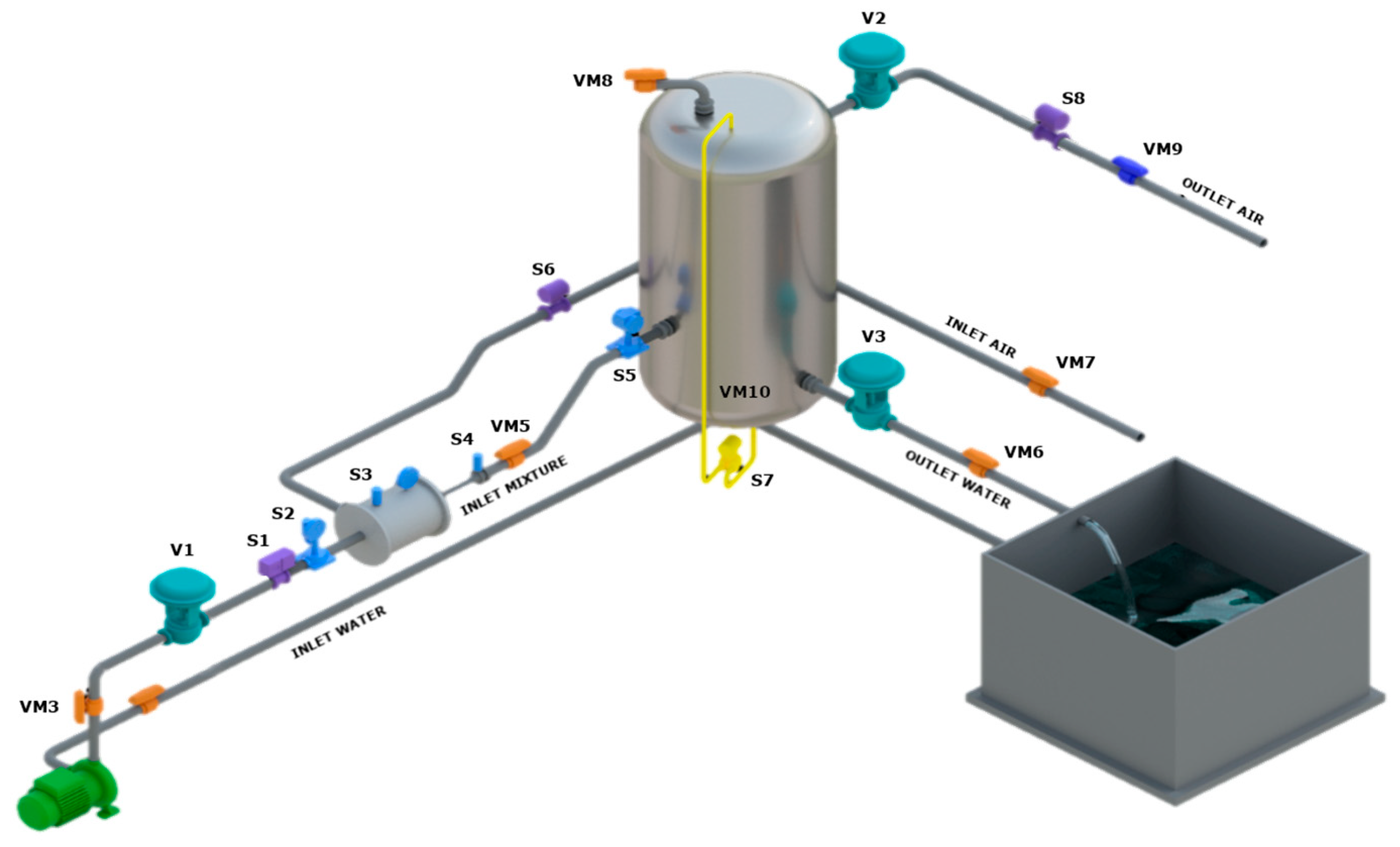
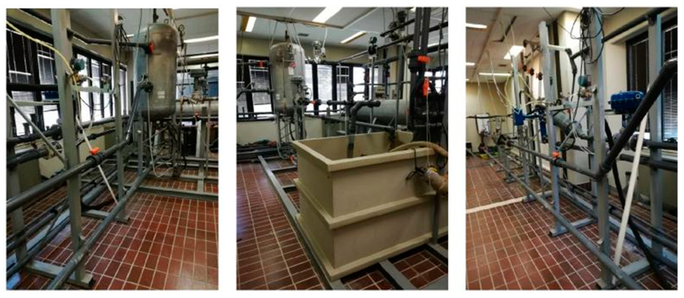
The two-phase experimental plant is located at the Department of Industrial Engineering and Mathematical Sciences (DIISM) of the Università Politecnica delle Marche (Ancona, Italy). The 3D plant model is shown in Figure 3, and some views of the actual plant are in Figure 4. It reproduces the extraction of oil and natural gas from depleted wells. Specifically, the useful life of hydrocarbon reservoirs is related to their potential and operating costs. A well is depleted if the water in it is in such quantities that it cannot be extracted or if the volumes of hydrocarbons produced become uneconomic considering the very high operating costs to make them unsustainable if there is little or no production. In such circumstances, the most obvious solution would be installing appropriate pumps located on the surface and at the base of the oil well with a very high cost compared to the produced hydrocarbon volumes. The system under consideration represents an undoubtedly more efficient solution. The extraction from a depleted reservoir is carried out by using the pressure of a hypothetical reservoir at the height of its useful life. Due to its physical characteristics, the latter’s pressure is higher than the transport pressure and, therefore, is able to create suction on the depleted reservoir, which, in contrast, does not have enough pressure for transport on the line.

Gas-liquid ejectors can mix two phases at different pressures (depletion and good wells) and impart the necessary transport energy. While in a realistic situation, the fluids treated are crude oil and natural gas, for safety reasons, water and ambient air are used in the case of the experimental plant. Specifically, water in a tank and a positive displacement pump model pressurized well behaviour, while ambient air simulates natural gas from a depleted reservoir. Pressurized water (“INLET WATER”) enters the ejector, creating a vacuum that draws in a certain amount of air from the environment (“INLET AIR”), thus creating a two-phase mixture (“INLET MIXTURE”). The resulting mixture is directed into a vertical tank that acts as a slug catcher to separate the liquid (“OUTLET WATER”) and gas (“OUTLET AIR”) phases. The plant is equipped with three pneumatic valves: to control the inlet water pressure (V1), regulate the pressure inside the tank (V2), and regulate the water level (V3). All the “VMs” in Figure 3 represent shut-off valves used to reproduce anomalies in the system.

Table 2. Plant equipment characteristics.

ID	Description	UM	Type	Tag
S1	Inlet water pressure	[bar]	OUTPUT	Endress+Hauser Cerabar M PMP51
S2	Inlet water flow rate	[m3/h]	OUTPUT	Endress+Hauser Promag W
S3	Ejector pressure	[bar]	OUTPUT	Setra 280E
S4	Diffuser mixture pressure	[bar]	OUTPUT	Foxboro 841GM CI1
S5	Tank pressure	[bar]	OUTPUT	Foxboro 841GM-CI1
S6	Inlet air flow rate	[m3/h]	OUTPUT	Foxboro Vortez DN 50
S7	Tank water level	[mm]	OUTPUT	Foxboro IDP-10
S8	Outlet air flow rate	[m3/h]	OUTPUT	Endress+Hauser Prowirl 200
V1	Valve 1 closure	[%]	INPUT	Spirax Sarco 9126E Pneumatic Valve
V2	Valve 2 closure	[%]	INPUT	ECKARDT MB6713 Pneumatic Valve
V3	Valve 3 closure	[%]	INPUT	ECKARDT MB6713 Pneumatic Valve

briefly describes the plant equipment characteristics in terms of the monitored variable, the unit of measurement, type of equipment, and finally, the equipment tag code. All the plant sensors and valves are connected to a Revolution Pi device to acquire their status value.

3.2. The Self-Organizing Map

The Self-Organizing Map (SOM) was first theorized by Kohonen [40]. Based on the similarity of the input information, the algorithm reorders the data in the map by performing a sort of classification. The structure of this artificial neural network consists only of the input and output layers.

The input dataset consists of a samples number equal to D described by n features, ${\mathrm{x}}_{\mathrm{i}}=\left({\mathrm{x}}_1,{\mathrm{x}}_2,\dots ,{\mathrm{x}}_{\mathrm{n}}\right)$ with $\mathrm{i}=1,2\dots \mathrm{D}$. Each features sample (${\mathrm{x}}_{\mathrm{i},\mathrm{j}}$ with j = 1, 2 … n) is associated with a weight vector in the output map ${\mathrm{w}}_{\mathrm{j}}^{\mathrm{i}}=\left({\mathrm{w}}_{\mathrm{j},1}^{\mathrm{i}},{\mathrm{w}}_{\mathrm{j},2}^{\mathrm{i}},\dots ,{\mathrm{w}}_{\mathrm{j},\mathrm{m}}^{\mathrm{i}}\right)$ where m is the number of output nodes. The initial weights, randomly initialized, must be close to zero, avoiding the presence of similar weights. This way, no order is imposed on the network during the initialization phase.

The output layer is a low-dimensional representation of the input data. Typically, its nodes are arranged in a two-dimensional architecture organized as a grid with a rectangular or hexagonal topology. Mainly, the number of output nodes denotes the maximum number of clusters and influences the accuracy of the SOM.

The scientific study of Shalaginov and Franke [41] can be exploited to calculate the number of nodes in the output grid. Considering D samples in the input database, Equation (1) describes the number of output nodes m.

$$\mathrm{m}=5\sqrt{\mathrm{D}}$$

(1)

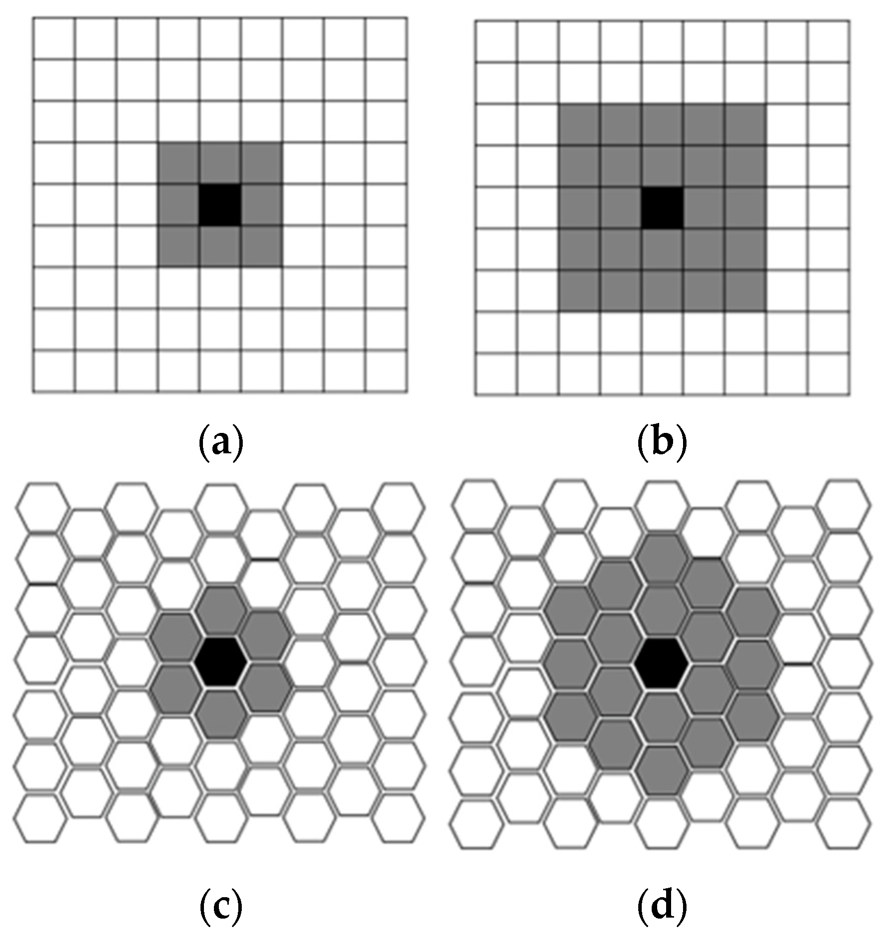
Once the number of output nodes is identified, choosing the proper grid topology is necessary. Indeed, each grid has specific properties: in the rectangular topology, each node has four neighbours, while in the hexagonal one, each node has six neighbours. In general, the hexagonal topology is the most used because of its more significant number of neighbours.

In unsupervised network learning, output nodes compete to be activated. Only the node with the weight closest to the input vector will be activated and declared the Best Matching Unit (BMU). Specifically, for the BMU identification, the distance between an input sample ${\mathrm{x}}_{\mathrm{i}}$ and all weight vectors ${\mathrm{w}}_{\mathrm{j}}$ is calculated using measurement methods such as Manhattan, Chebyshev, or Euclidean distance. However, according to Kohonen [40], the Euclidean distance (see Equation (2)) is the most suitable for a visual representation because a more isotropic visualization of the dataset is achieved.

$${\mathrm{d}}_{\mathrm{p}}^{\mathrm{i}}\left(\mathrm{k}\right)=\sqrt{\sum _{\mathrm{j}=1}^{\mathrm{n}}{({\mathrm{x}}_{\mathrm{i},\mathrm{j}}(\mathrm{k})-{\mathrm{w}}_{\mathrm{j},\mathrm{p}}^{\mathrm{i}}(\mathrm{k}))}^2}$$

(2)

With i = 1, 2 … D, p = 1, 2 … m, and k = 1, 2 … T, where T is the maximum iterations number. At iteration k, the winning node ${\mathrm{p}}_{\mathrm{i}}^{\mathrm{*}}\left(\mathrm{k}\right)$ of all those considered will be the one that minimizes Equation (2), as shown in Equation (3).

$${\mathrm{p}}_{\mathrm{i}}^{\mathrm{*}}\left(\mathrm{k}\right)=\arg \min \left\{{\mathrm{d}}_{\mathrm{p}}^{\mathrm{i}}\left(\mathrm{k}\right)\right\}$$

(3)

Likewise, human neurons process similar information using neighbouring neurons. The SOM’s topological organization requires that adjacent neurons represent inputs with similar properties in the output space. Therefore, the BMU determines the spatial position of cooperating nodes’ neighbourhoods. These nodes, sharing common characteristics, activate each other to learn something from the same input. This way, the BMU node and the neighbouring nodes weights must be adapted to become more representative and faithful to the input space. Two parameters must be set to achieve this step: the learning rate, α(k), and the neighbourhood size. In particular, the learning rate controls the change rate of the weights and the neighbourhood size at each iteration. Learning rate and neighbourhood size guarantee the algorithm convergence even after a reasonable number of iterations (at least 1000). Thus, the learning rate gradually decreases during network training. As described by Natita et al. [41], Equations (4)–(6) offer different learning rate formulas.

$$\mathsf{\alpha }\left(\mathrm{k}\right)=\mathsf{\alpha }(0)·\frac{1}{\mathrm{k}}$$

(4)

$$\mathsf{\alpha }\left(\mathrm{k},\mathrm{T}\right)=\mathsf{\alpha }(0)·(1-\frac{\mathrm{k}}{\mathrm{T}})$$

(5)

$$\mathsf{\alpha }\left(\mathrm{k},\mathrm{T}\right)=\mathsf{\alpha }(0)·{\mathrm{e}}^{\frac{\mathrm{k}}{\mathrm{T}}}$$

(6)

In particular, $\mathsf{\alpha }(0)$ is the value of the learning rate at the first iteration, and k is the current iteration. At this point, using a discrete-time formalism, let ${\mathrm{w}}_{\mathrm{j},{\mathrm{p}}^{\mathrm{*}}}^{\mathrm{i}}(\mathrm{k})$ be the weight vector of the winning node at iteration k. Then, at iteration k + 1, it is defined as described in Equation (7).

$${\mathrm{w}}_{\mathrm{j},{\mathrm{p}}^{\mathrm{*}}}^{\mathrm{i}}\left(\mathrm{k}+1\right)={\mathrm{w}}_{\mathrm{j},{\mathrm{p}}^{\mathrm{*}}}^{\mathrm{i}}\left(\mathrm{k}\right)+\mathsf{\alpha }\left(\mathrm{k}\right)·\left[{\mathrm{x}}_{\mathrm{i},\mathrm{j}}\left(\mathrm{k}\right)-{\mathrm{w}}_{\mathrm{j},{\mathrm{p}}^{\mathrm{*}}}^{\mathrm{i}}\left(\mathrm{k}\right)\right]$$

(7)

The topological properties of the initial space are preserved in the final one thanks to the neighbourhood size. The vectors of the nodes close to the BMU (${\mathrm{p}}_{\mathrm{i}}^{\mathrm{*}}\left(\mathrm{k}\right)$), indicated with ${\mathrm{N}}_{\mathrm{N}}^{\mathrm{*}}$, have a crucial role in the learning process. The rate of weights adaptation decreases moving away from the winning node, according to a decay function called the neighbourhood function, ${\mathrm{h}}_{{\mathrm{p}}^{\mathrm{*}},\mathrm{p}}(\mathrm{k})$, where ${\mathrm{p}}^{\mathrm{*}}$ indicates the winning node and $\mathrm{p}=1,2,\dots \mathrm{m}$. At this point, the weights of all other nodes can be updated according to Equation (8).

$${\mathrm{w}}_{\mathrm{j},\mathrm{p}}^{\mathrm{i}}\left(\mathrm{k}+1\right)={\mathrm{w}}_{\mathrm{j},\mathrm{p}}^{\mathrm{i}}\left(\mathrm{k}\right)+\mathsf{\alpha }\left(\mathrm{k}\right)·{\mathrm{h}}_{{\mathrm{p}}^{\mathrm{*}},\mathrm{p}}(\mathrm{k})·\left[{\mathrm{x}}_{\mathrm{i},\mathrm{j}}\left(\mathrm{k}\right)-{\mathrm{w}}_{\mathrm{j},\mathrm{p}}^{\mathrm{i}}\left(\mathrm{k}\right)\right]$$

(8)

Kohonen [40] claims that different types of neighbourhoods can be distinguished (Figure 5). A discrete neighbourhood function is defined as a function that defines a set ${\mathrm{N}}_{\mathrm{c}}$ of elements at the winning node, such as ${\mathrm{h}}_{{\mathrm{p}}^{\mathrm{*}},\mathrm{p}}(\mathrm{k})=\mathsf{\gamma }\left(\mathrm{t}\right)$ if $\mathrm{i}\in {\mathrm{N}}_{\mathrm{N}}^{\mathrm{*}}$ and ${\mathrm{h}}_{{\mathrm{p}}^{\mathrm{*}},\mathrm{p}}(\mathrm{k})=0$ if $\mathrm{i}\notin {\mathrm{N}}_{\mathrm{N}}^{\mathrm{*}}$. The γ(t) value indicates the degree of participation in weight update [42]. It is also possible to define the neighbourhood using a continuous function. The continuous neighbourhood function is often preferred over the discrete one because it decreases in time and space as the number of iterations increases. Thus, a more homogeneous output that preserves as much as possible the initial topological composition returns. There are several neighbourhood functions in the literature, such as the Bubble Equation (9), Gaussian Equation (10), Cutgass Equation (11), and Epanechikov Equation (12) [43].

$${\mathrm{h}}_{{\mathrm{p}}_{\mathrm{i}}^{\mathrm{*}}\mathrm{p}}\left(\mathrm{k}\right)=1(\mathrm{k})·(\mathsf{\sigma }\left(\mathrm{k}\right)-{\mathrm{d}}_{{\mathrm{p}}_{\mathrm{i}}^{\mathrm{*}}\mathrm{i}}^{\mathrm{i}})$$

(9)

$${\mathrm{h}}_{{\mathrm{p}}_{\mathrm{i}}^{\mathrm{*}}\mathrm{p}}\left(\mathrm{k}\right)=\exp \left(-\frac{{{\mathrm{d}}_{{\mathrm{p}}_{\mathrm{i}}^{\mathrm{*}}\mathrm{i}}^{\mathrm{i}}}^2}{2{\mathsf{\sigma }}^2\left(\mathrm{k}\right)}\right)$$

(10)

$${\mathrm{h}}_{{\mathrm{p}}_{\mathrm{i}}^{\mathrm{*}}\mathrm{p}}\left(\mathrm{k}\right)=\exp \left(-\frac{{{\mathrm{d}}_{{\mathrm{p}}_{\mathrm{i}}^{\mathrm{*}}\mathrm{i}}^{\mathrm{i}}}^2}{2{\mathsf{\sigma }}^2\left(\mathrm{k}\right)}\right)·1(\mathrm{k})·(\mathsf{\sigma }\left(\mathrm{k}\right)-{\mathrm{d}}_{{\mathrm{p}}_{\mathrm{i}}^{\mathrm{*}}\mathrm{i}}^{\mathrm{i}})$$

(11)

$${\mathrm{h}}_{{\mathrm{p}}_{\mathrm{i}}^{\mathrm{*}}\mathrm{p}}\left(\mathrm{k}\right)=\max \{0,1(\mathrm{k})-{\left(\mathsf{\sigma }\left(\mathrm{k}\right)-{\mathrm{d}}_{{\mathrm{p}}_{\mathrm{i}}^{\mathrm{*}}\mathrm{i}}^{\mathrm{i}}\right)}^2\}$$

(12)

${\mathrm{d}}_{{\mathrm{p}}_{\mathrm{i}}^{\mathrm{*}}\mathrm{i}}^{\mathrm{i}}$ indicates the distance between the BMU and the excited neuron i, 1(k) is the step function: 1(k) = 0 if k < 0 and 1(k) = 1 if k ≥ 0 and $\mathsf{\sigma }\left(\mathrm{k}\right)$ stands for the neighbourhood radius at iteration k. The maximum point of the symmetric Gaussian function is that defined by ${\mathrm{d}}_{{\mathrm{p}}_{\mathrm{i}}^{\mathrm{*}}\mathrm{i}}^{\mathrm{i}}=0$. Since it is a monotone decreasing function, Kohonen [40] suggests starting with a large $\mathsf{\sigma }\left(0\right)$ value since it has been seen experimentally that starting the training with too small a value does not bring the network to convergence.

3.3. Tuning Phase

Choosing the parameters that characterize the network, such as the neighbourhood size and the value of the learning rate, is a delicate operation. Indeed, these values cannot be chosen at first glance. Still, optimal values must be looked for in the space of possible variables to find a set of variables that will afford the algorithm the most desirable results [44]. Among the many hyper-parameterization techniques in the literature, the hyperopt.fmin function is chosen to find the optimal values of the SOM [45]. The task performed by this function is to find the best value of one or more scalar functions among a set of possible arguments. This method causes the user to describe the objective function space in which to search precisely in the optimal parameters of the network [46]. To use this function, it is necessary to define:

• The space on which to search.
• The objective function to be minimized.
• The database in which to store all search evaluations (optional).
• The search algorithm to be used (optional).

Equation (13) defines the search space consisting of the two linear distributions $\mathsf{\Phi }$ and $\mathrm{A}$. The first $\mathsf{\Phi }$ establishes a set of possible variable values the neighbourhood radius can take. At the same time, the $\mathrm{A}$ distribution indicates a potential deal to be assigned to the learning rate (Equations (15) and (16)). Finally, the sequence of values presented within a linear distribution is defined by a step (Equation (14)).

$$\mathrm{X}\left(\mathsf{\Phi },\mathrm{A}\right)$$

(13)

$$\mathrm{step}={10}^{-\mathsf{\mu }}\mathrm{with}\mathsf{\mu }\in \mathbb{N}\mathrm{and}\mathrm{step}\in (0,1]$$

(14)

$$\mathsf{\Phi }=\{\forall {\mathrm{s}}_{\mathrm{i}}\in ℝ:{\mathrm{s}}_{\mathrm{i}}=\mathrm{i}·\mathrm{s}\mathrm{t}\mathrm{e}\mathrm{p},\mathrm{i}\in [1,5\times {10}^{\mathsf{\mu }}],\mathrm{i}\in \mathbb{N}\}$$

(15)

$$\mathrm{A}=\{\forall {\mathrm{a}}_{\mathrm{i}}\in ℝ:{\mathrm{a}}_{\mathrm{i}}=\mathrm{i}·\mathrm{s}\mathrm{t}\mathrm{e}\mathrm{p},\mathrm{i}\in [1,5\times {10}^{\mathsf{\mu }}],\mathrm{i}\in \mathbb{N}\}$$

(16)

The task performed by hyper-parameterization is to test the SOM network with different learning rate values and neighbourhood size to find the best combination that minimizes an objective function (Equation (17)). In the case of SOM networks, it is necessary to have a low Quantization Error (QE). Only in this way can the map return outputs that preserve the topological relationships of the source data.

$${\mathrm{s}}_{\mathrm{i}}^{\prime },{\mathrm{a}}_{\mathrm{i}}^{\prime }=\mathrm{a}\mathrm{r}\mathrm{g}\mathrm{m}\mathrm{i}\mathrm{n}\left(\mathrm{Q}\mathrm{E}\right)$$

(17)

3.4. Quality of Self-Organizing Map

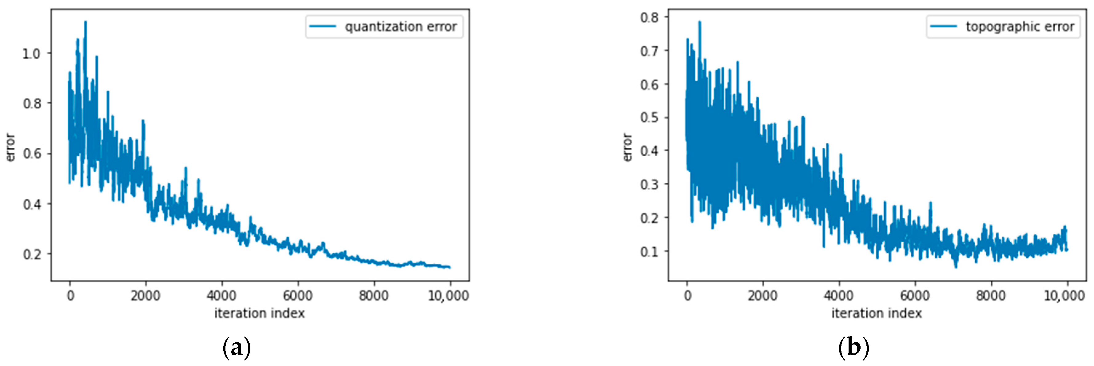
Several methods in the literature are used to validate the quality of the SOM. Pölzlbauer [47] validates the SOM according to two parameters concerning the quality of the network learning (Quantization Error, QE) and the quality of the projection of the source data onto the output map (Topographic Error, TE). At the end of the learning process, each input data $\mathrm{x}$ is assigned to a weight on the output map that best represents it ${\mathrm{w}}_{\mathrm{j},\mathrm{p}}^{\mathrm{i}}$ [48]. The difference $‖\mathrm{x}\left(\mathrm{k}\right)-{\mathrm{w}}_{\mathrm{j},\mathrm{p}}^{\mathrm{i}}\left(\mathrm{k}\right)‖$ between the input and its associated weight expresses the quantization error. Through Equation (18), it is possible to calculate the average quantization error, which numerically represents how similar the final map is to the initial dataset.

$$\mathrm{Q}\mathrm{E}=\frac{{\sum }_{\mathrm{k}=1}^{\mathrm{K}}‖\mathrm{x}\left(\mathrm{k}\right)-{\mathrm{w}}_{\mathrm{j},\mathrm{p}}^{\mathrm{i}}\left(\mathrm{k}\right)‖}{\mathrm{K}}$$

(18)

One way to reduce the value of QE is to increase the number of output nodes to have the samples distributed more sparsely over the map, but in this way, the direct correlation with TE would be lost. The quality of the data projection on the output map is determined by considering the Topographic Error (Equation (19)). This parameter defines the percentage of vectors for which the first and second BMUs are not adjacent. Equation (20) expresses how this value is calculated.

$$\mathrm{T}\mathrm{E}=\frac{1}{\mathrm{D}}\sum _{\mathrm{k}=1}^{\mathrm{D}}\mathrm{e}\mathrm{r}\mathrm{r}\left(\mathrm{x}\left(\mathrm{k}\right)\right)$$

(19)

$$\mathrm{err}\left(\mathrm{x}\left(\mathrm{k}\right)\right)=\left\{\begin{array}{ll}1,& \mathrm{if} {\mathrm{p}}_{\mathrm{i}}^{\mathrm{*}}\left(\mathrm{k}\right),2{\mathrm{p}}_{\mathrm{i}}^{\mathrm{*}}\left(\mathrm{k}\right)\in {\mathrm{N}}_{\mathrm{n}}^{\mathrm{*}}\\ 0,& \mathrm{otherwise}\end{array}\right.$$

(20)

After verifying the method and training the network, the input data are projected onto the output map. The nodes that make up the output grid accommodate only one class type, but sometimes this does not happen. Therefore, an analysis of cluster purity is conducted to uniquely assign a single class to each cell in the map [49]. Purity is a metric for how much a cluster contains a single class (Equation (21)). First, this parameter is calculated: count the number of data points from each cluster’s most common class type. Then, divide the total data points by the sum of all clusters. Formally, given a collection of clusters $\mathrm{M}$ and a set of classes $\mathrm{C}$, both splitting $\mathrm{N}$ data points, purity may be defined as:

$$\frac{1}{\mathrm{N}}\sum _{\mathrm{m}\in \mathrm{M}}\underset{\mathrm{c}\in \mathrm{C}}{\max }\left|\mathrm{m}\cap \mathrm{c}\right|$$

(21)

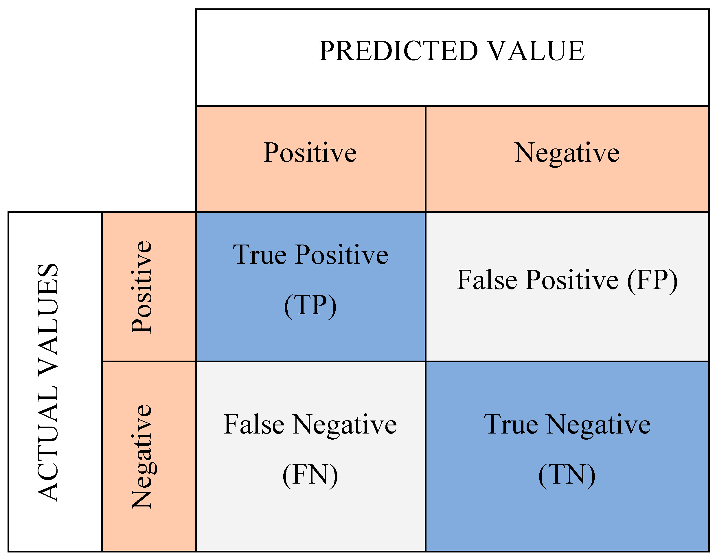
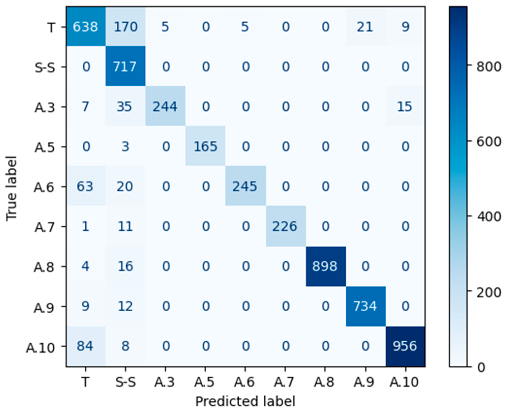
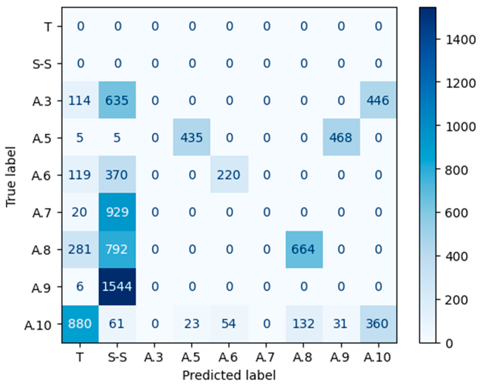
The confusion matrix is another tool to validate the results of the SOM Network [50]. A confusion matrix is a C × C matrix used to assess the effectiveness of a classification model, where C represents the number of target classes [51]. The matrix compares the actual goal values to the machine learning model’s predictions (Figure 6). Thus, this method evaluates a classification model’s performance by computing measures such as accuracy, precision, recall, and F1-score [34]. The parameters that make up the matrix are:

• True positives (TP): the actual value is positive, and the predicted is also positive.
• True negatives (TN): the actual value is negative, and the prediction is also negative.
• False positives (FP): the actual is negative, but the prediction is positive.
• False negatives (FN): the actual is positive, but the prediction is negative.

The following parameters can be exploited to analyse the properties of the confusion matrix:

• Accuracy (Equation (22))—is the percentage of samples in the test set that were categorized correctly.

  $$\mathrm{A}\mathrm{c}\mathrm{c}\mathrm{u}\mathrm{r}\mathrm{a}\mathrm{c}\mathrm{y}=\frac{\mathrm{T}\mathrm{P}+\mathrm{T}\mathrm{N}}{\mathrm{T}\mathrm{P}+\mathrm{F}\mathrm{P}+\mathrm{T}\mathrm{N}+\mathrm{F}\mathrm{N}}$$

  (22)
• Precision (Equation (23))—out of all the samples, how many belonged to the positive class compared to how many the model projected would.

  $$\mathrm{P}\mathrm{r}\mathrm{e}\mathrm{c}\mathrm{i}\mathrm{s}\mathrm{i}\mathrm{o}\mathrm{n}=\frac{\mathrm{T}\mathrm{P}}{\mathrm{T}\mathrm{P}+\mathrm{F}\mathrm{P}}$$

  (23)
• Recall (Equation (24))—the proportion of samples from the positive class was expected to do so.

  $$\mathrm{R}\mathrm{e}\mathrm{c}\mathrm{a}\mathrm{l}\mathrm{l}=\frac{\mathrm{T}\mathrm{P}}{\mathrm{T}\mathrm{P}+\mathrm{F}\mathrm{N}}$$

  (24)
• F1-Score (Equation (25))—the harmonic mean of the precision and recall scores obtained for the positive class.

  $$\mathrm{F}1-\mathrm{S}\mathrm{c}\mathrm{o}\mathrm{r}\mathrm{e}=\frac{2·\mathrm{P}\mathrm{r}\mathrm{e}\mathrm{c}\mathrm{i}\mathrm{s}\mathrm{i}\mathrm{o}\mathrm{n}·\mathrm{R}\mathrm{e}\mathrm{c}\mathrm{a}\mathrm{l}\mathrm{l}}{\mathrm{P}\mathrm{r}\mathrm{e}\mathrm{c}\mathrm{i}\mathrm{s}\mathrm{i}\mathrm{o}\mathrm{n}+\mathrm{R}\mathrm{e}\mathrm{c}\mathrm{a}\mathrm{l}\mathrm{l}}$$

  (25)

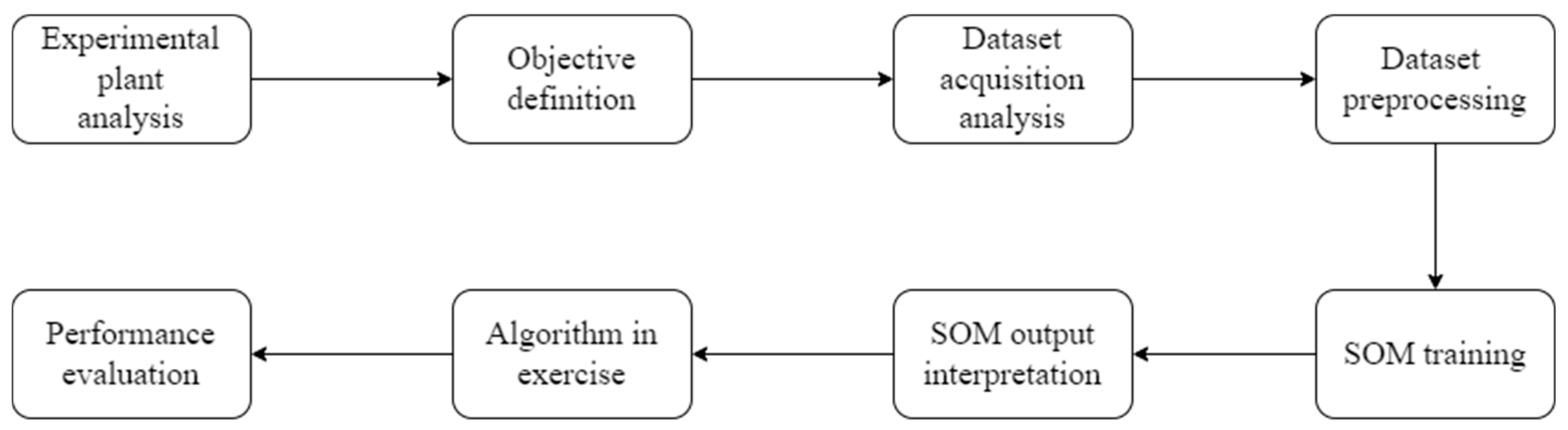
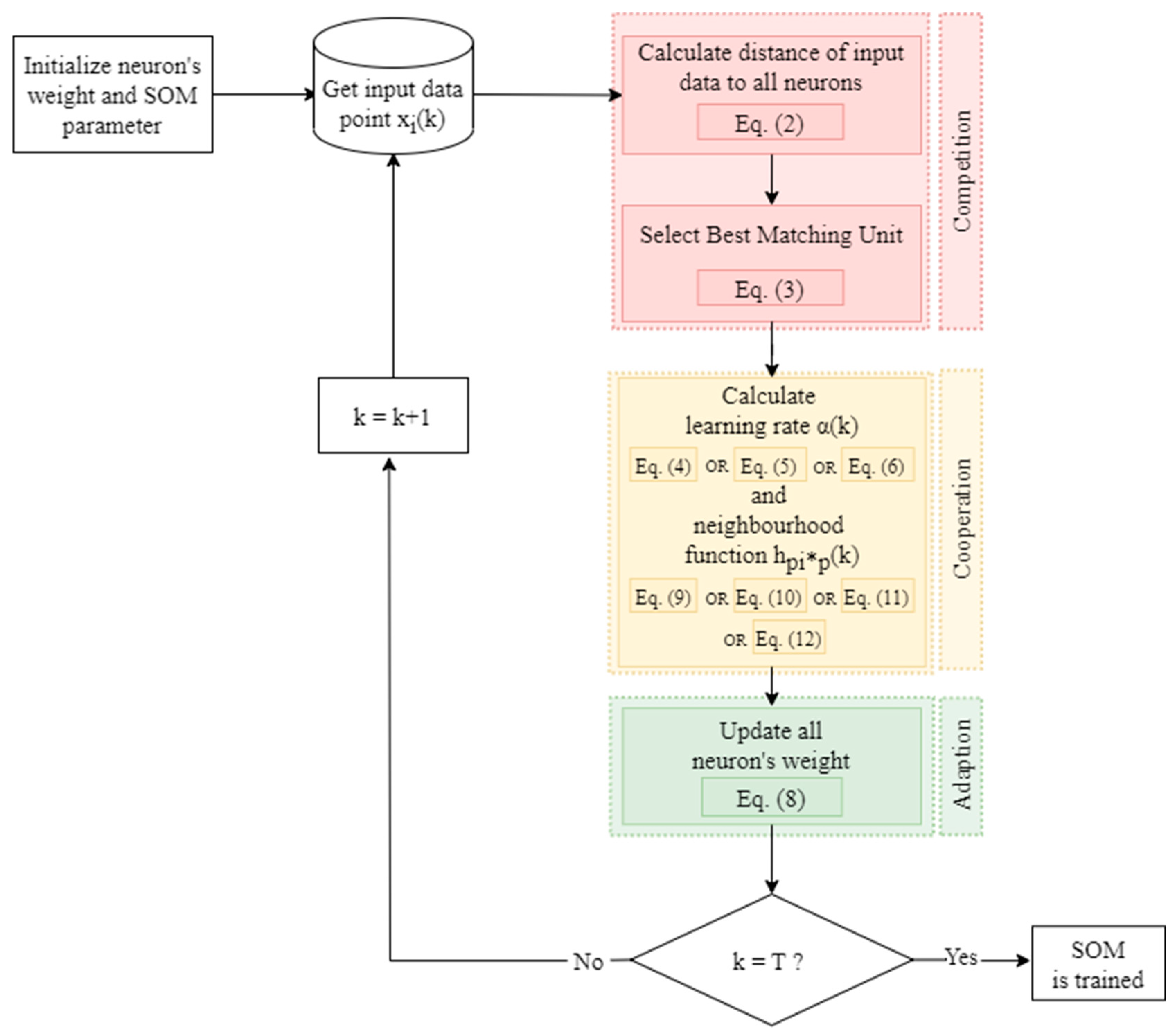
All the steps taken during the SOM algorithm’s training phase are depicted in a flowchart in Figure 7.

4. Results and Discussions

This section discusses the data collected by the plant. The steady-state and abnormal readings are managed within a single database representing the SOM network’s input. The data are projected onto the map and are validated depending on the quantization error. Finally, correlations between the identified and macro areas are analysed based on the data projected onto the map.

4.1. Raw Data Collection and Data Standardization

By acting on the pneumatic valve (V1, V2, and V3) closures and setting the inlet water pressure (S1) to 5.5 bar, the tank pressure (S5) to 1.3 bar, and the tank level (S7) to 300 mm, the standard plant behaviour has been achieved. Then, all the anomalies were reproduced by acting on the shut-off valve (VM) closures, as described in

Table 3. Description of the anomalies.

Test ID	Description
V10L1	It describes a minor tank water leakage obtained since closing the valve VM10 by 30%
V10L2	It describes a medium tank water leakage obtained since closing the valve VM10 by 60%
V10L3	It describes a grave tank water leakage obtained since closing the valve VM10 by 100%
V3L1	It describes a minor obstruction in the water inlet piping system obtained since closing the valve VM3 by 30%
V3L2	It describes a medium obstruction in the water inlet piping system obtained since closing the valve VM3 by 60%
V3L3	It describes a grave obstruction in the water inlet piping system obtained since closing the valve VM3 by 100%
V5L1	It describes a minor obstruction in the mixture inlet piping system obtained since closing the valve VM5 by 30%
V5L2	It describes a medium obstruction in the mixture inlet piping system obtained since closing the valve VM5 by 60%
V5L3	It describes a grave obstruction in the mixture inlet piping system obtained since closing the valve VM5 by 100%
V6L1	It describes a minor obstruction in the water outlet piping system obtained since closing the valve VM6 by 30%
V6L2	It describes a medium obstruction in the water outlet piping system obtained since closing the valve VM6 by 60%
V6L3	It describes a grave obstruction in the water outlet piping system obtained since closing the valve VM6 by 100%
V7L1	It describes a minor obstruction in the air inlet piping system obtained since closing the valve VM7 by 30%
V7L2	It describes a medium obstruction in the air inlet piping system obtained since closing the valve VM7 by 60%
V7L3	It describes a grave obstruction in the air inlet piping system obtained since closing the valve VM7 by 100%
V8L1	It describes a minor air leakage in the tank obtained since closing the valve VM8 by 30%
V8L2	It describes a medium air leakage in the tank obtained since closing the valve VM8 by 60%
V8L3	It describes a grave air leakage in the tank obtained since closing the valve VM8 by 100%
V9L1	It describes a minor obstruction in the air outlet piping system obtained since closing the valve VM9 by 30%
V9L2	It describes a medium obstruction in the air outlet piping system obtained since closing the valve VM9 by 60%
V9L3	It describes a grave obstruction in the air outlet piping system obtained since closing the valve VM9 by 100%

. The data are collected in a single database containing physical quantities of different types of different scales. Indeed, for each sampling, flow, pressure, and level measurements characterize the fluids circulating in the system. For this very reason, before starting the training phase of the SOM, the data are standardized through the z-score method, where a random variable X, with a mean $\mathsf{\gamma }$ and variance σ², is transformed to a random variable $\mathrm{Z}$ with mean 0 and variance equal to 1 [52]. The calculation involves subtracting from X, the variable of interest, its mean $\mathsf{\gamma }$ and dividing it by the standard deviation σ (Equation (26)).

$$\mathrm{Z}=\frac{\mathrm{X}-\mathsf{\mu }}{\mathsf{\sigma }}$$

(26)

4.2. The Algorithm

A computer equipped with a 12th Gen Intel(R) Core(TM) i9-12900KF 3.20 GHz processor, 32.0 GB RAM, and 16 GB GPU was used to perform the research work. The Self-Organizing map was written in Python code, and several libraries were used. NumPy and Pandas packages were needed to manipulate the data, while the MiniSom library was used for map creation and the Bokeh package for graphical representation. The MiniSom Function appears as follows:

$$\mathrm{SOM}=\mathrm{MiniSom}(\mathrm{x},\mathrm{y},\mathrm{input}\mathrm{len},\mathrm{topology},\mathrm{sigma},\mathrm{learning}\mathrm{rate},\mathrm{neighborhood}\mathrm{function},\mathrm{seed})$$

(27)

where $\mathrm{x}$ and $\mathrm{y}$ are the numbers of rows and columns of the output grid, $\mathrm{input}\mathrm{len}$ is the length of the database supplied to the network, $\mathrm{topology}$ defines the topology of the grid (rectangular or hexagonal), $\mathrm{sigma}$ is the initial radius of the neighbourhood, $\mathrm{learning}\mathrm{rate}$ represents the $\mathsf{\alpha }(0)$, $\mathrm{neighborhood}\mathrm{function}$ is Equation (10), and the $\mathrm{seed}$ is the seed of the network.

The readings from the steady-state test and all the Level 3 anomalies are collected in a database of 5321 samples. To improve readability and ensure a homogeneous output, the number of rows and columns in the output map was set to be equal, resulting in a square map. Applying the formula explained in Section 3.2 to the spatial dimension of the map, it is also possible to calculate these last two parameters. There are 18 rows and columns of the output map.

In function (27), the hexagonal topology is set for the grid cells, the inverse learning rate function is chosen (Equation (5)), the Gaussian neighbourhood function is imposed (Equation (10)), and the seed is also set to 0 to realize an isotropic, repeatable map that preserves the initial topological relationships.

The algorithm is hyper-parametrized for the optimal choice of parameters characterizing the learning rate and neighbourhood size. In Equation (14), $\mathsf{\mu }$ is set to 4 for both linear distributions. Therefore, the range $[1, 5\times {10}^{\mathsf{\mu }}]$ in Equations (15) and (16) is composed of 50,000 values, and the algorithm tests the SOM network by combining all possible values between these two distributions.

The input parameters to the network are defined as follows:

• x: 18.
• y: 18.
• Input len: 5130.
• Topology: hexagonal.
• Sigma: 2.382866878925671.
• Learning rate: 2.422871364551101.
• Neighbourhood function: Gaussian Function.
• Seed: 0

4.3. Validation

After setting the various parameters within the MiniSom Function, it is necessary to initialize the weights and start training the network. The weights associated with each output node are initialized randomly to small values close to zero, and the number of iterations is set to 10,000. Before visually studying the output map, it is necessary to validate the network according to the quantization and topographic errors. The quantization error allows us to assess the quality of network learning and shows how well the map fits the source data. This parameter is calculated by determining the average distance of the sample vectors to the BMU. The closer the error is to zero, the higher the quality of the map and the more correctly arranged the output data. Topographic error defines the percentage of vectors for which the first and second BMUs are not adjacent. A sample for which these two nodes are not adjacent counts as an error. If the topographic error is 0, no error has occurred. If it is 1, the topology was not preserved for any of the samples, and relationships from the input dataset are lost in the output map. As shown in Figure 8, both parameters tend to zero so the well-trained network preserves in the output map the topological relationships present in the source dataset.

Before studying the results obtained from projecting the input data into the output map, it is essential to analyse the U-Matrix (Unified Distance Matrix). This matrix contains the various Euclidean distances between the input data and its associated weight. Through the study of the U-Matrix, an initial analysis of the potential clusters in the map is possible. In Figure 9a, the U-Matrix is represented using a heat map. If the node’s colour is lighter, that node has similar properties to neighbouring nodes. On the other hand, if the colour is dark blue, that node has different characteristics from the neighbouring node. Eight clusters are visible while doing an initial qualitative study of the map’s colour tones, which the artificial intelligence programme projects the input data into.

4.4. Output Map

After an initial analysis of the U-Matrix, it is possible to analyse the matrix of occurrences of BMU responses (Figure 9b) through a colour map. In this case, dark-coloured boxes indicate those nodes that are recalled the most during the training phase and vice versa for the light-coloured boxes. The most responsive nodes have coordinates [5, 10] and [6, 10]. As shown in Figure 10, all readings of the system’s steady state are placed in these two locations. Unlike all other samples in the anomaly tests, the system’s steady-state samples always present the same trend and do not vary its state. Therefore, all steady-state readings are projected at those two nodes.

The nodes that make up the output grid accommodate only one class type, but sometimes this does not happen. Therefore, an analysis of cluster purity (Equation (21)) is conducted to uniquely assign a single class to each cell in the map. First, the purity value is calculated for each cell. Then, the overall purity value considers all cell purities. The overall value is 0.90, which means that statistically, the algorithm assigns each cell only one class 90% of the time. In conclusion, each node in the output map is assigned a class based on the purity of the clusters and the values provided by the U-Matrix. Figure 11 represents the final output map, where each cell has been filled with the colour of the specific category, as shown in

Table 4. Legend of SOM output map.

System State	Type of Anomaly	Tag	Colour
Transient of steady state	/	Hex	Fuchsia
Steady state	/	Asterisk	Orange
Anomaly 3 L3	Water	Dot	Green
Anomaly 5 L3	Air-water	Dot	Red
Anomaly 6 L3	Water	Dot	Purple
Anomaly 7 L3	Air	Dot	Brown
Anomaly 8 L3	Air	Cross	Pink
Anomaly 9 L3	Air	Line	Gray
Anomaly 10 L3	Tank	Rhombus	Yellow

.

The first readings of almost all anomaly tests are clustered near the regime area. Then, the shut-off valves are closed manually, and the system goes from a steady state to a new operating point. Indeed, the database provided to the network also contains the readings that characterize the transient of each abnormal test. The shut-off valves VM3 and VM6 impede the passage of water into the system and out of the tank. The SOM can recognize a water anomaly in the system in both cases and projects the readings in the left part of the map. The VM7 valve prevents air inflow, VM9 prevents air outflow, and VM8 simulates an air leak inside the tank. The algorithm recognizes that all three anomalies involve air and arranges the readings in the right part of the map. The red area shown in Figure 12 collects all the readings recorded on the system when the VM5 valve impedes the passage of the two-phase air-water fluid into the tank. The algorithm arranges these anomalous readings under the area marking the water anomaly and the air anomaly area. Finally, the yellow area (Figure 12) in the lower right collects the readings recorded on the system when a water leakage from the tank through the VM10 valve is simulated. The diversity of this anomaly from the others described above prompts the SOM to arrange the readings in a new area set in the lower right corner.

From the study conducted on the output map, the algorithm arranges the input data into six macro areas (Figure 12): (i) steady-state area (orange), (ii) water anomaly macro-area (green), (iii) air-water anomaly area (red), (iv) tank anomaly area(yellow), (v) air anomaly macro-area (blue sky), and (vi) steady-state transition area (fuchsia).

4.5. Input Data Confusion Matrix

As explained in Section 3.4, each node provided to the algorithm contains a particular system state. Therefore, since nine classes are supplied to the input, the confusion matrix is 9 × 9 (Figure 13).

Table 5. Classification report of the level 3 anomalies.

	Precision	Recall	F1-Score	Support
Transient of Steady State	0.79	0.75	0.77	848
Steady State	0.72	1.00	0.84	717
Anomaly 3	0.98	0.81	0.89	301
Anomaly 5	1.00	0.98	0.99	168
Anomaly 6	0.98	0.75	0.85	328
Anomaly 7	1.00	0.95	0.97	238
Anomaly 8	1.00	0.98	0.99	918
Anomaly 9	0.97	0.97	0.97	755
Anomaly 10	0.98	0.91	0.94	1048

collects all the parameters needed for analysis. The lowest precision value (0.72) is assigned to the class representing the steady state. Filtering the projected data on the output map shows that the steady-state area contains all the first anomalous test readings. The reason why this result appears is that the anomaly test data are not acquired automatically. The shut-off valves are mechanical. In addition, proper coordination is needed between the operator who turns on the acquisition system and the operator who rotates the shut-off valve obstructing the flow.

Figure 14 displays all the airflow sensor output values from every experiment. The data are standardized, and the different tests are divided according to the colours shown in Table 4. The black dots indicate the samples in the node [6,10]. This result is confirmed further by the fact that when the shut-off valve is triggered, the system needs some time to migrate to a new operating point. Consequently, the first measurements obtained during anomaly tests often reflect the transition of the system from a steady state to anomaly state.

The overall accuracy of the algorithm is 90%, so the network optimally classifies the readings in the output map.

4.6. The Algorithm Evaluation

In the second phase of the research work, level 1 and level 2 anomalous readings are analysed on the output map. As performed previously, the level 1 and level 2 outlier test data were first unified and then standardized with the mean and variance of the input dataset. Figure 15 represents all readings of levels 1 and 2 projected onto the output map.

The green circles in Figure 15a represent the level 1 and 2 anomaly readings generated by the VM3 shut-off valve. The new input data are arranged in four distinct clusters. The first two clusters are projected close to the border of the green area and the edge of the orange-coloured steady state. The readings of the first two levels of VM3 are similar to those of these two clusters. The last two clusters represent the readings of level 2. They are placed within the area of the reservoir anomaly since the system in both situations has the same incoming water flow rate.

The red area on the map represents the cluster in which the source network distributes the anomalous readings of the system caused by the occlusion of the pipe connecting the ejector outlet to the inlet of the holding tank. Level 1 and level 2 anomaly test data from the VM5 valve are shown using red circles. These new input data, recording lower occlusions than level 3, are distributed to the sides of the red area. The first readings of anomaly 5 level 1 deviate from the red area board and are located at the board of the air anomaly macro area (Figure 15b).

The purple circles represent the data from the level 1 and level 2 anomalous tests of the VM6 shut-off valve. Again, the new data are projected into the edge of the corresponding anomalous area since, once more, the occlusions are less severe than those of level 3 (Figure 15c).

The brown circles depict the first two degrees of occlusion generated by the VM7 shut-off valve on the output map. The data recorded from these two tests show a reduced obstruction of the air intake duct. The system is ready and immediately returns to the steady-state condition; this is why level 1 and 2 readings are projected between the brown and orange areas of the steady-state data (Figure 15d).

The network separates the data from levels 1 and 2 of anomaly 8 into four major clusters, each symbolized by a pink cross. Due to their reduced intensity, all level 1 measurements are projected near the regime data zone. Level 2 measures, on the other hand, are situated close to the edge of the anomaly 8 level 3 region and have a bigger valve opening (Figure 15e).

By providing the algorithm with data from levels 1 and 2 of anomaly 9, all readings are projected into three clusters marked with a grey line. In addition, because the occlusions are smaller than those in level 3, the data are also projected near to the regime zone, notably in the transient zone. (Figure 15f).

The VM10 manual shut-off valve simulates the loss of water from the tank. The yellow area of the map at the bottom right contains the level 3 VM10 readings. The map shows the network level 1 and 2 readings as separate clusters of yellow rhombi positioned throughout the network. Even slightly opening VM10 makes the system unstable and prevents it from finding a new equilibrium point. While level 1 readings, due to their lower intensity, are projected to be close to the regime zone, level 2 readings are projected to be close to the yellow area (Figure 15g).

Moreover, the confusion matrix is used to verify the effectiveness of the algorithm. Figure 16 represents the confusion matrix, and

Table 6. Classification report of the level 1 and 2 anomalies.

	Precision	Recall	F1-Score	Support
Anomaly 3	0.00	0.00	0.00	1195
Anomaly 5	0.95	0.48	0.63	913
Anomaly 6	0.80	0.31	0.45	709
Anomaly 7	0.00	0.00	0.00	949
Anomaly 8	0.83	0.38	0.52	1737
Anomaly 9	0.00	0.00	0.00	1550
Anomaly 10	0.48	0.23	0.31	1541

compiles the findings after sending the network level 1 and 2 anomaly values as input.

A closer look at the data on the confusion matrix reveals that many samples of level 1 and level 2 anomalies are misclassified. Most readings are projected in the steady-state area and some in the transient area. Thus, the occlusion intensity is too low.

The VM3 shut-off valve prevents water from entering the system. Therefore, this anomaly will only affect the system when the valve is entirely closed. The reason is that if the valve is not entirely closed, it can allow water through, regardless of the amount of water the system needs. For precisely this reason, the algorithm recognizes level 1 and level 2 anomaly 3 values as steady-state measurements when supplied.

However, the new tests for anomaly 5 show the highest accuracy level at 95 per cent. Even by slightly closing the inlet water flow shut-off valve at the tank, the system enters a new state that differs significantly from the steady state, and it is like level 3.

The results obtained from anomaly 6 level 1 and 2 data projection are also good. The accuracy reaches 80% because even if the VM6 valve is closed a little, the flow rate of water leaving the tank is like that of level 3.

Anomaly tests of inlet and outlet air produce the lowest accuracy values. In these two scenarios, even with valves VM7 and VM9 partially closed, air still enters and exits the system without experiencing a real occlusion. Figure 17 depicts the inlet air flow rate relative to the steady state for testing anomaly 7 levels 1 and 2. Figure 18 shows the air output for the tests of anomaly 9 level 1 and level 2 compared to the steady state.

The two figures attest that the trend of the anomalous air system is very similar to the trend of the steady state under both circumstances.

In conclusion, despite the low-precision results, the algorithm can still evaluate system conditions. The created model can classify the presence or absence of an anomaly. For example, suppose there is a significant occlusion in the system pipelines. In that case, the algorithm can identify and classify it, but if there is only a minor occlusion, the model can only notify the problem.

4.7. Summary

Self-Organizing Maps are generally used to solve clustering problems such as image classification [53] or customer segmentation in the economic-financial domain [54]. In the case of this study, the SOM algorithm is applied to anomaly detection instead. The proposed algorithm can ensure reliable performance in detecting and classifying anomalies in the experimental two-phase system.

The readings with which the algorithm was trained describe six distinct macro-areas on the output map: the steady-state area, the transient area, the water anomaly area, the air anomaly area, the air-water two-phase fluid anomaly area, and the reservoir leakage anomaly area. Given that the algorithm has an overall accuracy of 90%, the network efficiently classifies the readings on the output map.

Once the algorithm is trained using steady-state test data and level 3 anomalies, it maps the output for data obtained from level 1 and level 2 anomalous tests. However, the accuracy of these tests is lower compared to the training data since the pipe obstructions created during these tests are of lower intensity. As a result, in most cases, the readings from level 1 and 2 anomalous states are projected into the transient area.

Apart from its ease of implementation, the algorithm generates an easily comprehensible output map, even for individuals not well versed in artificial neural networks. Moreover, if the algorithm is connected to the Digital Twin of the experimental system, it would enable real-time projection of the system data onto the output map. Consequently, if the system were to be in a condition different from the steady state, it would be easy to identify the anomaly type, as the readings would be mapped onto the relevant anomaly area.

Two conclusions can be drawn from the output map if an anomaly is detected. Firstly, the more severe the obstruction, the further the map will project the reading towards the centre of the region of interest. Secondly, if the obstruction is minimal, the data will be displayed at the border of the area.

However, the analysed case study highlighted a limitation in characterizing the transient region. The algorithm can alert us that the system is no longer in steady-state conditions but cannot classify the detected anomaly type. To describe the transient area more thoroughly, one could study how the network organizes readings recorded on the system when multiple anomalies are combined simultaneously. In addition, these new tests could make a more detailed analysis of the macro-output areas boundaries.

5. Conclusions

The purpose of the paper was to implement a Self-Organizing Map to monitor the health of the two-phase air-water plant within the Department of Industrial Engineering and Mathematical Sciences (DIISM) of the Università Politecnica delle Marche (Ancona, Italy).

This algorithm is an example of unsupervised learning, which is advantageous because it does not require the user to label the training data manually. Moreover, the SOM algorithm offers the benefit of decreasing the dimensionality of the input dataset to yield an output that is simple to interpret. The input dataset is multidimensional and consists of readings from all the flow, level, and pressure sensors directly connected to the experimental system during various tests. In contrast, the output of the algorithm is a two-dimensional map that is easy to interpret, even for an operator who is not an expert in artificial neural networks. The algorithm implemented in this research has an accuracy of 90%. It can identify the state of the two-phase system by associating a particular state with each node on the output map. The output map comprises six macro-areas representing the possible states of the two-phase system. Thus, the operator can quickly identify the state of the plant by observing which area the system reading is projected onto. If the system deviates from normal operating conditions, the system reading will be projected into the anomaly area of the output map, allowing the operator to pinpoint the location of the fault within the system.

The research study has identified certain limitations. The first constraint pertains to the synchronization of data acquisition on the system. Anomaly tests are conducted by manually closing the shut-off valves to generate obstructions in the line to create the training dataset. However, there is often a lack of synchronization between the operator closing the valve and the one initiating the recording. To overcome this limitation in future research, replacing manual valves with solenoid valves is being considered to have complete control over the system and reduce acquisition errors. Another limitation is associated with the anomalies of air at level 1 and level 2. When these two types of anomalies are recorded, the readings in the output map are projected close to the steady-state and transient areas. This is because, in such scenarios, the system behaviour is very similar to that of the steady-state state. In the next research work, it will be necessary to discriminate these anomalous areas more efficiently to generate a detailed map.

In addition, in the transient area, the algorithm cannot accurately identify the type of anomaly but only indicates that the system is no longer in steady-state conditions. New readings will be recorded in the upcoming research work to overcome this limitation by combining multiple anomalies in the same test. This method may enable the study of individual boundaries of the output macro-areas in greater detail.

References

1. Barari, A.; Tsuzuki, M.S.G. Smart Manufacturing and Industry 4.0. Appl. Sci. 2023, 13, 1545. [Google Scholar] [CrossRef]
2. Iamsumang, C.; Mosleh, A.; Modarres, M. Monitoring and learning algorithms for dynamic hybrid Bayesian network in on-line system health management applications. Reliab. Eng. Syst. Saf. 2018, 178, 118–129. [Google Scholar] [CrossRef]
3. Di Carlo, F.; Mazzuto, G.; Bevilacqua, M.; Ciarapica, F. Retrofitting a Process Plant in an Industry 4.0 Perspective for Improving Safety and Maintenance Performance. Sustainability 2021, 13, 646. [Google Scholar] [CrossRef]
4. Tiddens, W.; Braaksma, J.; Tinga, T. Decision Framework for Predictive Maintenance Method Selection. Appl. Sci. 2023, 13, 2021. [Google Scholar] [CrossRef]
5. Mazzuto, G.; Antomarioni, S.; Ciarapica, F.E.; Bevilacqua, M. Health Indicator for Predictive Maintenance Based on Fuzzy Cognitive Maps, Grey Wolf, and K-Nearest Neighbors Algorithms. Math. Probl. Eng. 2021, 2021, 8832011. [Google Scholar] [CrossRef]
6. Converso, G.; Gallo, M.; Murino, T.; Vespoli, S. Predicting Failure Probability in Industry 4.0 Production Systems: A Workload-Based Prognostic Model for Maintenance Planning. Appl. Sci. 2023, 13, 1938. [Google Scholar] [CrossRef]
7. Zornio, P.; Boudreaux, M. Case Study: How Digital Transformation Paved the Way for One Refinery’s Predictive Maintenance Strategy. In Proceedings of the Offshore Technology Conference, Houston, TX, USA, 6–9 May 2019. [Google Scholar] [CrossRef]
8. Lian, Y.; Geng, Y.; Tian, T. Anomaly Detection Method for Multivariate Time Series Data of Oil and Gas Stations Based on Digital Twin and MTAD-GAN. Appl. Sci. 2023, 13, 1891. [Google Scholar] [CrossRef]
9. Bevilacqua, M.; Ciarapica, F.E.; Mazzuto, G. A Fuzzy Cognitive Maps Tool for Developing a RBI&M Model. Qual. Reliab. Eng. Int. 2014, 32, 373–390. [Google Scholar] [CrossRef]
10. Luo, R.; Sheng, B.; Lu, Y.; Huang, Y.; Fu, G.; Yin, X. Digital Twin Model Quality Optimization and Control Methods Based on Workflow Management. Appl. Sci. 2023, 13, 2884. [Google Scholar] [CrossRef]
11. Huang, J.; Pham, D.T.; Wang, Y.; Qu, M.; Ji, C.; Su, S.; Xu, W.; Liu, Q.; Zhou, Z. A case study in human–robot collaboration in the disassembly of press-fitted components. Proc. Inst. Mech. Eng. Part B J. Eng. Manuf. 2019, 234, 654–664. [Google Scholar] [CrossRef]
12. Wanasinghe, T.R.; Wroblewski, L.; Petersen, B.; Gosine, R.G.; James, L.A.; De Silva, O.; Mann, G.K.I.; Warrian, P.J. Digital twin for the oil and gas industry: Overview, research trends, opportunities, and challenges. IEEE Access 2020, 8, 104175–104197. [Google Scholar] [CrossRef]
13. Bevilacqua, M.; Bottani, E.; Ciarapica, F.E.; Costantino, F.; Di Donato, L.; Ferraro, A.; Mazzuto, G.; Monteriù, A.; Nardini, G.; Ortenzi, M.; et al. Digital Twin Reference Model Development to Prevent Operators’ Risk in Process Plants. Sustainability 2020, 12, 1088. [Google Scholar] [CrossRef] [Green Version]
14. Pierdicca, R.; Prist, M.; Monteriù, A.; Frontoni, E.; Ciarapica, F.; Bevilacqua, M.; Mazzuto, G. Augmented Reality Smart Glasses in the Workplace: Safety and Security in the Fourth Industrial Revolution Era. In Lecture Notes in Computer Science (Including Subseries Lecture Notes in Artificial Intelligence and Lecture Notes in Bioinformatics; Springer: Berlin/Heidelberg, Germany, 2020; Volume 12243, pp. 231–247. [Google Scholar] [CrossRef]
15. Chen, T.; Sampath, V.; May, M.C.; Shan, S.; Jorg, O.J.; Martín, J.J.A.; Stamer, F.; Fantoni, G.; Tosello, G.; Calaon, M. Machine Learning in Manufacturing towards Industry 4.0: From ‘For Now’ to ‘Four-Know’. Appl. Sci. 2023, 13, 1903. [Google Scholar] [CrossRef]
16. Zunino, C.; Valenzano, A.; Obermaisser, R.; Petersen, S. Factory Communications at the Dawn of the Fourth Industrial Revolution. Comput. Stand. Interfaces 2020, 71, 103433. [Google Scholar] [CrossRef]
17. Selvik, J.T.; Bellamy, L.J. Addressing human error when collecting failure cause information in the oil and gas industry: A review of ISO 14224:2016. Reliab. Eng. Syst. Saf. 2020, 194, 106418. [Google Scholar] [CrossRef]
18. Pech, M.; Vrchota, J.; Bednář, J. Predictive Maintenance and Intelligent Sensors in Smart Factory: Review. Sensors 2021, 21, 1470. [Google Scholar] [CrossRef]
19. Wu, Y.; Zhao, H.; Zhang, C.; Wang, L.; Han, J. Optimization analysis of structure parameters of steam ejector based on CFD and orthogonal test. Energy 2018, 151, 79–93. [Google Scholar] [CrossRef]
20. Zio, E. Prognostics and Health Management (PHM): Where are we and where do we (need to) go in theory and practice. Reliab. Eng. Syst. Saf. 2022, 218, 108119. [Google Scholar] [CrossRef]
21. Chen, C.L.P.; Zhang, C.-Y. Data-intensive applications, challenges, techniques and technologies: A survey on Big Data. Inf. Sci. 2014, 275, 314–347. [Google Scholar] [CrossRef]
22. Koroteev, D.; Tekic, Z. Artificial intelligence in oil and gas upstream: Trends, challenges, and scenarios for the future. Energy AI 2021, 3, 100041. [Google Scholar] [CrossRef]
23. Li, H.; Yu, H.; Cao, N.; Tian, H.; Cheng, S. Applications of Artificial Intelligence in Oil and Gas Development. Arch. Comput. Methods Eng. 2021, 28, 937–949. [Google Scholar] [CrossRef]
24. Mazzuto, G.; Antomarioni, S.; Marcucci, G.; Ciarapica, F.E.; Bevilacqua, M. Learning-by-Doing Safety and Maintenance Practices: A Pilot Course. Sustainability 2022, 14, 9635. [Google Scholar] [CrossRef]
25. Redutskiy, Y.; Camitz-Leidland, C.M.; Vysochyna, A.; Anderson, K.T.; Balycheva, M. Safety systems for the oil and gas industrial facilities: Design, maintenance policy choice, and crew scheduling. Reliab. Eng. Syst. Saf. 2021, 210, 107545. [Google Scholar] [CrossRef]
26. Mohammed, A. Data driven-based model for predicting pump failures in the oil and gas industry. Eng. Fail. Anal. 2023, 145, 107019. [Google Scholar] [CrossRef]
27. Naseri, M.; Baraldi, P.; Compare, M.; Zio, E. Availability assessment of oil and gas processing plants operating under dynamic Arctic weather conditions. Reliab. Eng. Syst. Saf. 2016, 152, 66–82. [Google Scholar] [CrossRef] [Green Version]
28. Antomarioni, S.; Ciarapica, F.E.; Bevilacqua, M. Association rules and social network analysis for supporting failure mode effects and criticality analysis: Framework development and insights from an onshore platform. Saf. Sci. 2022, 150, 105711. [Google Scholar] [CrossRef]
29. Quatrini, E.; Costantino, F.; Di Gravio, G.; Patriarca, R. Machine learning for anomaly detection and process phase classification to improve safety and maintenance activities. J. Manuf. Syst. 2020, 56, 117–132. [Google Scholar] [CrossRef]
30. Zainuddin, Z.E.; Akhir, A.P.; Hasan, M.H. Predicting machine failure using recurrent neural network-gated recurrent unit (RNN-GRU) through time series data. Bull. Electr. Eng. Inform. 2021, 10, 870–878. [Google Scholar] [CrossRef]
31. Wang, H.; Chen, S. Insights into the Application of Machine Learning in Reservoir Engineering: Current Developments and Future Trends. Energies 2023, 16, 1392. [Google Scholar] [CrossRef]
32. Choubey, S.; Karmakar, G.P. Artificial intelligence techniques and their application in oil and gas industry. Artif. Intell. Rev. 2021, 54, 3665–3683. [Google Scholar] [CrossRef]
33. Gupta, D.; Shah, M. A comprehensive study on artificial intelligence in oil and gas sector. Environ. Sci. Pollut. Res. 2022, 29, 50984–50997. [Google Scholar] [CrossRef] [PubMed]
34. Aljameel, S.S.; Alomari, D.M.; Alismail, S.; Khawaher, F.; Alkhudhair, A.A.; Aljubran, F.; Alzannan, R.M. An Anomaly Detection Model for Oil and Gas Pipelines Using Machine Learning. Computation 2022, 10, 138. [Google Scholar] [CrossRef]
35. Mazzuto, G.; Ciarapica, F.E.; Ortenzi, M.; Bevilacqua, M. The Digital Twin Realization of an Ejector for Multiphase Flows. Energies 2021, 14, 5533. [Google Scholar] [CrossRef]
36. Barbariol, T.; Feltresi, E.; Susto, G.A. Machine Learning approaches for Anomaly Detection in Multiphase Flow Meters. IFAC-PapersOnLine 2019, 52, 212–217. [Google Scholar] [CrossRef]
37. Mohammed, A.S.; Anthi, E.; Rana, O.; Saxena, N.; Burnap, P. Detection and mitigation of field flooding attacks on oil and gas critical infrastructure communication. Comput. Secur. 2023, 124, 103007. [Google Scholar] [CrossRef]
38. Breiman, L. Random forests. Mach. Learn. 2001, 45, 5–32. [Google Scholar] [CrossRef] [Green Version]
39. Khoei, T.T.; Kaabouch, N. A Comparative Analysis of Supervised and Unsupervised Models for Detecting Attacks on the Intrusion Detection Systems. Information 2023, 14, 103. [Google Scholar] [CrossRef]
40. Kohonen, T. The self-organizing map. Proc. IEEE 1990, 78, 1464–1480. [Google Scholar] [CrossRef]
41. Natita, W.; Wiboonsak, W.; Dusadee, S. Appropriate Learning Rate and Neighborhood Function of Self-organizing Map (SOM) for Specific Humidity Pattern Classification over Southern Thailand. Int. J. Model. Optim. 2016, 6, 61–65. [Google Scholar] [CrossRef] [Green Version]
42. Reutterer, T.; Natter, M. Segmentation-based competitive analysis with MULTICLUS and topology representing networks. Comput. Oper. Res. 2000, 27, 1227–1247. [Google Scholar] [CrossRef]
43. Hoomod, H.K.; Al-Mejibli, I.; Jabboory, A.I. Efficient Neighborhood Function and Learning Rate of Self-Organizing Map (SOM) for Cell Towers Traffic Clustering. J. Al-Qadisiyah Comput. Sci. Math. 2017, 9, 122–130. [Google Scholar] [CrossRef]
44. Probst, P.; Boulesteix, A.L.; Bischl, B. Tunability: Importance of Hyperparameters of Machine Learning Algorithms. arXiv 2018, arXiv:1802.09596. Available online: http://arxiv.org/abs/1802.09596 (accessed on 14 March 2023).
45. Bassi, D.; Singh, H. A Comparative Study on Hyperparameter Optimization Methods in Software Vulnerability Prediction. In Proceedings of the 2nd International Conference on Computational Methods in Science & Technology (ICCMST), Mohali, India, 17–18 December 2021. [Google Scholar] [CrossRef]
46. Bergstra, J.; Komer, B.; Eliasmith, C.; Yamins, D.; Cox, D.D. Hyperopt: A Python library for model selection and hyperparameter optimization. Comput. Sci. Discov. 2015, 8, 014008. [Google Scholar] [CrossRef]
47. Pölzlbauer, G. Survey and Comparison of Quality Measures for Self-Organizing Maps. In Proceedings of the Fifth Workshop on Data Analysis, Vysoké Tatry, Slovakia, 24–27 June 2004; Elfa Academic Press: Vysoké Tatry, Slovakia, 2004; pp. 67–82. [Google Scholar]
48. Dresp-Langley, B.; Wandeto, J. Human Symmetry Uncertainty Detected by a Self-Organizing Neural Network Map. Symmetry 2021, 13, 299. [Google Scholar] [CrossRef]
49. Arockiam, A.J.M.S.; Irudhayaraj, E.S. Reclust: An efficient clustering algorithm for mixed data based on reclustering and cluster validation. Indones. J. Electr. Eng. Comput. Sci. 2022, 29, 545–552. [Google Scholar] [CrossRef]
50. Jaiswal, A.; Kumar, R. Stochastic Self-Organizing Map and Proposed Enlarge C4.5 to Diagnose Breast Cancer. In Proceedings of the 2022 2nd International Conference on Advance Computing and Innovative Technologies in Engineering, ICACITE, Greater Noida, India, 28–29 April 2022; pp. 582–587. [Google Scholar] [CrossRef]
51. Kulkarni, A.; Chong, D.; Batarseh, F.A. Foundations of data imbalance and solutions for a data democracy. In Data Democracy: At the Nexus of Artificial Intelligence, Software Development, and Knowledge Engineering; Academic Press: Cambridge, MA, USA, 2020; pp. 83–106. [Google Scholar] [CrossRef]
52. Gustafsson, J.; Sandin, F. District heating monitoring and control systems. In Advanced District Heating and Cooling (DHC) Systems; Woodhead Publishing: Sawston, UK, 2015; pp. 241–258. [Google Scholar] [CrossRef]
53. Amitrano, D.; Di Martino, G.; Iodice, A.; Riccio, D.; Ruello, G. Urban Area Mapping Using Multitemporal SAR Images in Combination with Self-Organizing Map Clustering and Object-Based Image Analysis. Remote Sens. 2022, 15, 122. [Google Scholar] [CrossRef]
54. Wang, C. Efficient customer segmentation in digital marketing using deep learning with swarm intelligence approach. Inf. Process. Manag. 2022, 59, 103085. [Google Scholar] [CrossRef]
Figure 1. Oil and gas documents by year.
Applsci 13 03725 g001
Figure 2. The research approach.
Applsci 13 03725 g002
Figure 3. The experimental plant 3D model.
Applsci 13 03725 g003
Figure 4. Some views of the experimental plant.
Applsci 13 03725 g004
Figure 5. Different discrete neighbourhood functions with different grid types. (a,b) Rectangular SOM Grid; (c,d) Hexagonal SOM Grid.
Applsci 13 03725 g005
Figure 6. Confusion matrix for the binary classification [51].
Applsci 13 03725 g006
Figure 7. All steps of the SOM artificial neural network.
Applsci 13 03725 g007
Figure 8. Parameters for network validation: (a) quantization error; (b) topographic error.
Applsci 13 03725 g008
Figure 9. SOM Colour map: (a) U-Matrix Colour Map; (b) activation response map.
Applsci 13 03725 g009
Figure 10. The output map of input data. The figure legend can be consulted in Table 4.
Applsci 13 03725 g010
Figure 11. All classes predicted by the SOM algorithm. The color legend can be consulted in Table 4.
Applsci 13 03725 g011
Figure 12. Macro-areas in the output map.
Applsci 13 03725 g012
Figure 13. Input data confusion matrix.
Applsci 13 03725 g013
Figure 14. Airflow sensor readings and samples in the box [6,10]. The color legend can be consulted in Table 4.
Applsci 13 03725 g014
Figure 15. Output map for level 1 and level 2 anomalies samples. (a) Anomalies 3 L1, L2; (b) anomalies 5 L1, L2; (c) anomalies 6 L1, L2; (d) anomalies 7 L1, L2; (e) anomalies 8 L1, L2; (f) anomalies 9 L1, L2; (g) anomalies 10 L1, L2. The color legend can be consulted in Table 4.
Applsci 13 03725 g015aApplsci 13 03725 g015b
Figure 16. Levels 1 and 2 confusion matrix.
Applsci 13 03725 g016
Figure 17. Inlet air flow rate of steady state, anomaly 7 level 1 and 2 samples.
Applsci 13 03725 g017
Figure 18. Outlet air flow rate of steady state, anomaly 9 level 1 and 2 samples.
Applsci 13 03725 g018