Article

Explainable AI for Machine Fault Diagnosis: Understanding Features’ Contribution in Machine Learning Models for Industrial Condition Monitoring

Dipartimento di Ingegneria Meccanica e Aerospaziale (DIMEAS), Politecnico di Torino, Corso Duca Degli Abruzzi 24, 10129 Torino, Italy
*
Author to whom correspondence should be addressed.
Appl. Sci. 2023, 13(4), 2038; https://doi.org/10.3390/app13042038
Submission received: 30 December 2022 / Revised: 19 January 2023 / Accepted: 1 February 2023 / Published: 4 February 2023

Abstract

:
Although the effectiveness of machine learning (ML) for machine diagnosis has been widely established, the interpretation of the diagnosis outcomes is still an open issue. Machine learning models behave as black boxes; therefore, the contribution given by each of the selected features to the diagnosis is not transparent to the user. This work is aimed at investigating the capabilities of the SHapley Additive exPlanation (SHAP) to identify the most important features for fault detection and classification in condition monitoring programs for rotating machinery. The authors analyse the case of medium-sized bearings of industrial interest. Namely, vibration data were collected for different health states from the test rig for industrial bearings available at the Mechanical Engineering Laboratory of Politecnico di Torino. The Support Vector Machine (SVM) and k-Nearest Neighbour (kNN) diagnosis models are explained by means of the SHAP. Accuracies higher than 98.5% are achieved for both the models using the SHAP as a criterion for feature selection. It is found that the skewness and the shape factor of the vibration signal have the greatest impact on the models’ outcomes.

1. Introduction

One of the most important components of modern industry is rotating machinery [1]. Rolling element bearings are one of the essential parts of these machines, because they provide stiff support with a low-power consumption, thanks to their overall low friction coefficient, in a wide range of operating conditions [2]. They are also the most critical component, because they are susceptible to many failure causes not only related to wear and fatigue, but also to faulty installation, poor maintenance, and bad handling practices [3,4,5]. Their damage and consequent failure can cause significant unexpected downtimes, economic losses, and safety-related issues [6,7]. Therefore, in the past few decades, industries have recognised the importance of a reliable and robust condition monitoring (CM) system for fault detection and diagnosis [8,9].
Rolling element bearings are complex mechanical systems, in which the interaction between their elements produces vibrations even if they are “geometrically perfect”, and the presence of faults, defects, and their location produce a characteristic impulsive vibration signature [10]. Thus, vibration analysis has become one of the most used techniques in CM, because the signal acquired from the machine contains clear fault-related signatures and can be explored easily through signal processing techniques [11,12,13,14,15,16]. In most situations the bearing vibration cannot be measured directly, so the vibration signature is affected by noise coming from the structure and other equipment in the system. For that reason, machine users would prefer an automatic method to shorten the maintenance cycle and improve the diagnosis accuracy, which is called intelligent fault diagnosis (IFD). This technique uses machine learning (ML) theories and algorithms, such as the support vector machine (SVM) [17,18,19,20,21], the k-nearest algorithm (kNN) [22,23], artificial neural networks (ANNs) [24,25], deep belief networks (DBNs) [26], and convolutional neural networks (CNNs) [27,28,29], for fault classification [30]. A database of vibration data is used to extract some important and characteristic features to train the ML algorithms at the recognition of faults. Features can be extracted from the time, frequency, or time–frequency domain, but high-dimension feature vectors may contain either redundant or irrelevant information that can increase the computational cost and reduce the accuracy of the classification algorithm [31]. Indeed, overfitting problems correlated to high-dimensional data can deteriorate the performance of ML algorithms, since their generalisability decreases as the number of features increases [32]. Thus, feature selection, with a dimensionality-reduction technique, plays a fundamental role in designing powerful and robust AI algorithms [33]. Then, unlike physics-based models, explaining the contribution given by each feature to the outcome of an IFD model is not straightforward.
The term “feature importance” refers to a set of strategies for allocating scores to input features in a predictive model, indicating the relative significance of each item when producing a prediction [34]. Commonly used feature selection algorithms for bearing fault diagnosis include the following:
  • Filter-based methods: filters directly pre-process the collected features depending on the data intrinsic characteristics (correlation between features and class label), independent to the training of the algorithm. Typical importance indicators are Relief and Relief-F [35], information gain (IF) [36], Minimum Redundancy Maximum Relevance [37], Fischer score [38], and Distance Evaluation (DE) [39];
  • Wrapper-based methods: wrappers evaluate the interaction of the feature selection activity with the training phase of classifiers [40,41];
  • Embedded methods: feature selection is performed during the classification process by adding an L1 [42] or L2 [43] regularisation term in the cost function, making the computation faster than that of the wrappers.
Other widely used data-compression techniques are the principal component analysis (PCA) [44], the linear discriminant analysis (LDA) [45], and the partial least square (PLS) [46], which are based on an algebraic calculation and geometric projection to create the separability into the feature space. However, these approaches lack an appropriate explanation of the feature selection process and a proper justification about the influence of each feature on the final output of the IFD. Without a proper understanding of the feature selection process, all the ML-based classifiers only focus on the classification accuracy, such as the black box approach [9].
The SHAP (SHapley Additive exPlanations) value [47] is a novel feature importance calculation method, which is suitable for both regression and classification problems that can represent a valid alternative to the most used feature selection methods, because it can provide a local interpretation of the model on a single prediction, as well as the global average behaviour of the model in terms of the contribution of each feature to the outcome of the ML algorithm [48].According to the existing literature [9,49,50,51], the terms “interpretability” and “explainability” are often used synonymously, referring to models where users can understand how the inputs are mapped into outputs. This is the case for the techniques aimed at quantifying the contribution given by each feature to determine the outcome of their importance and highlight those with the greatest impact on prediction. In recent years, the SHAP value has become a popular method for the interpretation of the feature contributions in fitted ML models, as it can be seen in the references [47,52,53,54,55,56,57], posing the bases to Explainable Artificial Intelligence (XAI) [58] and new feature selection methods.

1.1. Literature Review

A review of the existing literature about Shapley values shows that the researches from Strumbelj et al. [55,59] were the first to propose them in the explanation of how features contribute to the prediction of classification and regression machine learning algorithms, posing the basis for XAI. They showed that Shapley values can reveal the influence of features, no matter the concept that the AI algorithm learns. An issue that affected all the algorithms based on the Shapley values was the high computational cost, but Song et al. [52] proposed a solution to make the computation feasible, even for a large number of input data and features, by sampling the permutations of the inputs randomly and estimating the cost functions related to the evaluated algorithms via the Monte Carlo simulation. The work by Lundberg et al. [47] introduced the kernel SHAP framework, which involved the standard Shapley value algorithm and the local interpretable model-agnostic explanation (LIME) algorithm, to assign each feature an importance value for a particular prediction. Further developments of the SHAP method were carried out by Aas et al. [53], who introduced the extension to the kernel SHAP to reduce the computation time and lead to more reliable predictions when features are correlated. Redelmeier et al. [56], who developed an algorithm able to explain the contribution of mixed (continuous, discrete, and categorical) and dependent features using conditional inference trees, and reported an improvement in the computation time when the features are dependent, with respect to Aas et al.
The kernel SHAP and the extension to the kernel SHAP were successfully used in studies regarding many different subjects to explain the outcome of both classifiers and the regression ML algorithms. Banerjee et al. [60] used the Shapley values to find causal connections between socioeconomic metrics and the spread of COVID-19 in the different phases of the pandemic. Vega Garcia et al. [34] applied the SHAP method to explain the forecasts of the air quality in terms of the NO2 concentration made by the long short-term memory (LSTM) deep learning model, while Rohmer et al. [61] explained the predictions of a machine-learning-based model for sea-level projections. The SHAP method can also be applied to finance, as it was performed in the study by Moehle et al. [57], who wanted to assess the feature importance in the evaluation of the portfolio performance to genomics. This is similar to the work by Watson et al. [62], who explained the importance of interpretable machine learning (iML) for making the prediction of the ML algorithm understandable to human, when the observed phenomena are highly complex and dependent on a large number of variables, and to aviation, as cited in the research by Midftfjord et al. [63]. They employed the SHAP method to highlight the most important features affecting the outcome of the XGBoost algorithm for the real-time evaluation of the airport runway conditions. The SHAP method can also be used for the multi-label classification problem, as it was reported in Dong et al. [64] and Goštautaite et al. [65]: the former proposed and tested a multi-label learning fused with the Shapley value (SHAPFS-ML), while the latter used the SHAP method to explain the predictions about the students’ learning style. The SHAP explanation was also used in medicine (Chen et al. [66], Oh et al. [67]), psychology (Akimoto et al. [68], Li et al. [69]), and engineering (Sun et al. [70], Remman et al. [71])
In the field of feature selection, the research from Cohen et al. [72] was the first to present contribution selection algorithms (CSAs) that were based on Shapley values to select the most relevant features. The CSA was tested on seven different datasets and the authors reported its capability to improve the performance of their classifier, competing with the most used feature selection methods, especially in those cases where features interacted with each other. Marcilio et al. [73] stated that the absolute of the SHAP values can be extrapolated to be used as a feature selection mechanism, while providing a human-compatible explanation for the predictions of ML algorithms. However, they reported that the kernel SHAP approach takes a quadratic amount of time in both the dimensionality and size of the dataset, making the computation unfeasible even for moderate datasets, but they concluded that this problem could be decreased by selecting features based on correlation before feeding the SHAP algorithm. Zacharias et al. [74] developed a design framework of an XAI-based feature selection method that evaluates the performance of a ML model with a reduced number of features, selected depending on their SHAP values, with respect to the original one, which is trained considering all the features. They highlighted that the use of XAI for feature selection may make the task more accessible for intermediate data scientists and might thereby contribute to data democratisation, facilitating the exchange of information between ML developers and domain experts to enhance the effectiveness of feature selection. This kind of algorithm was employed by Guha et al. [75] in a ML model for visual human action recognition and by Jothi et al. [76] for a ML model predicting generalised anxiety disorder among women. They both reported a high improvement in the computation time of their models after feature selection, proving the validity of that method. A further development was proposed by Tripathi et al. [77] who developed a feature selection algorithm that was based on the SHAP values for a binary classification problem, which does not need a user-defined threshold on the importance values or the number of important features.
There are reports in the literature about the application of the SHAP method to explain the outcomes of ML classifying algorithms for fault detection in rotating machinery. The SHAP algorithm was applied to supervised learning in the works by Hasan et al. [9], who explained the decisions of a kNN classifier for a small-sized ball bearing fault diagnosis, highlighting the most relevant features and concluding that the presented model had a better generalisation capability than the standard algorithm, making it perform a bearing fault diagnosis under different configurations and working conditions. Mey et al. [78] explained that the prediction of deep neural networks applied to the fault diagnosis of rotating systems through the analysis of vibration data. On the other hand, Brito et al. [49] explained the outputs of an unsupervised machine learning algorithm for fault detection in rotating machinery with gears and employed the Shapley values in a fault diagnosis to find the root causes of the faults.

1.2. Scope of the Research and Outline

In the field of IFD that is related to rotating machinery, only few works deal with the SHAP value as an instrument to assess the importance of features [9,17,49,78,79]. Additionally, the literature presents no evidence of XAI analysis performed for industrial applications characterised by medium-sized bearings and the assessment of the effects of SHAP-based feature selection on the testing accuracy of classifying algorithms. To the best of the authors’ knowledge, this is the first work dealing with this topic for industrial cases, involving medium-sized spherical roller bearings for high-duty applications.
For that reason, the present work is aimed at investigating the capabilities of the SHAP method to analyse feature contributions, making their selection univocally justifiable and trackable to achieve more robust and reliable ML algorithms for IFD of industrial bearings in rotating machinery for industrial interest. To this aim, specific experimental activities were conducted on the test rig for medium-sized industrial bearings available at the Mechanical Engineering Laboratory of Politecnico di Torino [80].
This paper is organised as follows: The introduction provides and overview of IFD and XAI by exploring the existing literature. Additionally, the aim of this work is described. The second section provides insight into the theoretical arguments underlying SVM, kNN, and Shapley values. The third section describes the test rig and the experimental activity conducted on medium-sized bearings. Section 4 includes the application of the SHAP analysis to the trained IFD models, whereas the fifth section provides the results and discussion on the explainability of diagnosis models and feature selection abilities. Finally, the sixth section includes the concluding remarks.

2. Theoretical Background

This section introduces the Artificial Intelligence (AI) tools that are employed in this study for the IFD and interpretability of AI models. Namely, the SVM and the kNN algorithms are selected among the ML models, whereas the SHAP technique is employed for interpreting the diagnosis that is achieved through the black box models.

2.1. ML Models

AI algorithms for fault diagnoses of rotating machinery have become popular due to their robustness and adaptation capabilities The first and most traditionally used algorithms for fault diagnosis are the SVM and kNN [30].

2.1.1. Support Vector Machines (SVMs)

A SVM is a supervised learning AI algorithm developed by Cortes and Vapnik [81] that is widely used in classification tasks and can manage large feature spaces, because the dimension of the classified vectors used for the training phase does not have an influence on the performance. Thus, the SVM is a good approach for fault diagnosis, since the vibration features might not have to be limited. It has good generalisation properties, because in the goal of the training phase is the minimisation of the Structural Misclassification Risk (SMR) [82,83,84]. The SMR is an inductive principle of use in ML, which was introduced by Vapnik and Chervonenkis [85] and is implemented through the minimisation of the expression reported in Equation (1):
E t r a i n + λ   H w  
where E t r a i n is the training error, λ is the constant regularisation term, H is the regularisation function that controls the trade-off between minimising the training error and minimising the expected gap between the training and test errors, and w is the vector containing the weight of each feature.
Thus, the cost function J of the algorithm can be written as reported in Equation (2):
J w = 1 2 N i = 1 N h w x i y i 2 + λ 2 j = 1 d w j 2  
where N is the number of examples in the database, x the vector of the feature values related to the i-th example, h w is the predicting function of the classifier, y is the label of the i-th example, d is the number of features, and w is the j-th entry of the vector of weights.
Given the set of input data reported in Equation (3),
D = x 1 , y 1 , , x N , y N             i = 1 , , N  
which are labelled depending on the class ( y i = ± 1 ) . The linear SVM theory supposes that there exists a hyperplane that represent the boundary between classes. The hyperplane is expressed in Equation (4),
w T   x + b = 0  
where b is a constant scalar term.
The maximisation of the margin distance between the points and the decision hyperplanes provides some reinforcement to the algorithm, making the classification of new points simpler [86].
Considering the possible presence of noise in data with the slack variable ζ i and the error penalty constant C , the optimal hyperplane that separates the data can be obtained as a solution to the optimisation problem of Equation (5):
minimize       1 2 w 2 + C i = 1 N ζ i s . t .         y i w T   x i + b = 0 1 ζ i ,         i = 1 , , N ζ i 0 ,                                                                                           i = 1 , , N  
Replacing the weight vector w with w = i = 1 N α i y i x i , where α is the weight of the i-th sample, the optimisation problem can be written in the form of Equation (6):
f x = sign i , j = 1 N α i y i ( x i x j ) + b  
SVMs can also be used in nonlinear classification problems that apply kernel functions, which map the d -dimensional input vector x into a l -dimensional feature space to make a linear classification feasible. Using the non-linear vector function K x i , x j = Φ T x i   Φ x j , the decision function can be written in the form of Equation (7):
f x = sign i , j = 1 N α i y i ( Φ T x i   Φ x j ) + b  
The kernel function of the following Equation (8) returns the dot product of the feature space mapping from the original data points:
K x i , x j = Φ T x i   Φ x j  
There are many types of kernel functions, such as linear, polynomial, and Gaussian RBF (radial basis function). The selection of the most suitable kernel is crucial, because it defines the feature space in which the training set data will be classified [20,82].

2.1.2. k-Nearest Neighbour (kNN)

The kNN algorithm is a non-parametric, supervised learning method developed by Fix and Hodges [87], in which the input is made of the k closest training samples of a dataset and the output for a classification problem is a class membership: the object is assigned to the class most common among its k nearest neighbours. Given a set of observations D ,
D = x 1 , y 1 , , x N , y N             i = 1 , , N  
where x i is the feature vector and y i is the corresponding class label of the i-th example. The x i , y i is assumed to be i.i.d. from some unknown distribution P of ( x , y ) on R d × ω 1 , , ω M , where M is the number of classes, and the goal is the design of a classifying function ϕ n   :   R d ω 1 , , ω M that maps a feature vector x into its desired class from ω 1 , , ω M .
The performance of the classifier is evaluated through the probability error of Equation (10) [88]:
J ϕ n = P x , y :   ϕ n x y  
where J is the cost function and ϕ n   is the classifying function.
If the underlying distribution is known, then the optimal decision rule ϕ * that minimises the probability of error is the Bayes decision rule of Equation (11):
ϕ * x = arg max P ( y | x )  
It can be shown that at any given point, x , the probability that its nearest neighbour x belongs to class ω i converges to the corresponding a posteriori probability P ( ω i | x ) as the number of reference observations goes to infinity. It was shown by Cover and Hart [89] that under some continuity conditions on the underlying distribution, the asymptotic probability of error L N N for a multi-class kNN classifier is bound by the terms reported in Equation (12):
L * L N N L * 2 M M 1 L *  
where L * is the optimal Bayes probability of error. Thus, the nearest-neighbour rule is asymptotically optimal when the classes are not overlapping [90].
In the classification phase, after the constant k has been defined by the user, an unlabelled vector is classified by assigning the label that is most frequent among the k training samples that are nearest to that query point. The distance metric could be represented by the Euclidean distance, the Hamming distance, or the correlation coefficients. The value of k deeply affects the classification performance [40]: larger values reduce the effects of noise but make the boundaries between classes less distinct. The accuracy is also affected by the presence of noisy or irrelevant features, or if the feature scales are not consistent with their importance. Finally, data-reduction is one of the biggest problems when working with huge datasets, because only some of the data points, called prototypes, are needed for accurate classification. A commonly used algorithm for dataset reduction is the Hart algorithm [91].

2.2. Shapley Values

The Shapley values [92] were introduced to assign pay-outs to players depending on their contribution towards the total playout, but they can be effectively used to measure the global importance of a feature. Shapley values can be explained by using the game theory as follows: given a cooperative game with d players aiming at maximising a payoff and letting S M = 1 , , d be a subset of S players, the contribution function ν S , which maps a subset of players to the real number, called the contribution of coalition S , describes the total expected sum of payoffs that the member of S can obtain by cooperation. Thus, Shapley values embody a method to distribute the total gains to players. The amount that player j earns is given by Equation (13) [53]:
ϕ j ν = ϕ j = S M \ j S ! d S 1 ! d ! ( ν ( S j ) ν S ) ,     j = 1 , , d  
This expression is a weighted mean over the contribution functions differences for all subsets S of players not containing player j . The algorithm also accounts for the non-distributed gain ϕ 0 = ν .
In the ML theory, single predictions take the place of a pay-out, and features become the players. The main properties of the Shapley values can be summarised as follows [93].
  • Efficiency: the total gain is distributed j = 0 d ϕ j = ν M ;
  • Symmetry: if i and j are two players that contribute equally to all coalitions, then their Shapley value is the same ν S i = ν S j ϕ i = ϕ j ;
  • Dummy player: if a player does not contribute to any coalitions, then his Shapley value is zero ϕ j = 0 ;
  • Monotonicity: if two games v and v and a player always makes a greater contribution to v than to v for all S , then the gain for v will be greater than that for v   ν S i v S ν S i v S   S     ϕ i v ϕ i v ;
  • Linearity: if two coalition games described by the gain functions v and w are combined, the distributed gain is the sum of the two gains is ϕ j v + w = ϕ j v + ϕ j w . This is valid also for a multiplication by a constant value α , ϕ j α   v = α   ϕ j v .
Given a training set of N labelled samples D = x 1 , y 1 , , x N , y N   used to train a predictive ML model f x whose outcome should be as close as possible to label y , Shapley values can be used to explain the prediction y * = f x * for a specific feature vector x = x * . The prediction can be written as reported in Equation (14):
f x * = ϕ 0 + j = 1 d ϕ j *  
where ϕ 0 = E f x and ϕ j * is the ϕ j for x = x * .
Therefore, Shapley values explain the difference between the prediction y * = f x * and the global average prediction. For the computation of the Shapley values for a prediction explanation, the contribution v S for a certain subset S must be defined. This function should take values similar to f x * when only the value of the subset S of these features is known. As cited by Lundberg [47], the expected output of the predictive model of Equation (15), conditional to the feature values x S = x S * of this subset, can be used:
v S = E [ f x | x S = x S * ]  
Thus, the conditional expectation summarises the whole probability distribution and, if it is considered the prediction for f x * , it is also the minimiser of the squared error loss function.
There are two main algorithms for the computation of the Shapley: the KernelSHAP and the extension to the KernelSHAP method. Both define the value function of Equation (16) such that the sum of the Shapley values of a query point over all the features corresponds to the total deviation of the prediction for the query point from an average:
j = 1 d ϕ j ν S = f x E f x  
Their main difference is in the way the feature contribution to the final prediction is evaluated: the latter is an interventional method, which attributes an influence onto x j only if the value function that is computed and considering that element is significantly different than if it was computed without it. On the contrary, the conditional approach of the former attributes even influences features with no interventional effect, only because of their presence in the model. Thus, this kind of approach requires further modelling of how the features are correlated [94].
The extension to the KernelSHAP algorithm [53] defines the value function of Equation (17) of the feature in S at the query point x using the conditional distribution of X S C , given that X S is the query point values:
ν S = E X S C | X S = x S f x S , X S C  

3. Dataset for Industrial Bearings

The dataset employed in this study was constructed by means of the test rig for industrial medium-sized bearings available at the Mechanical Engineering Laboratory of Politecnico di Torino [80]. The test rig was specifically designed for research activities. A comprehensive description of the test rig is provided in the reference [80]. The dataset involves ten shaft speeds, three different radial loads, and three bearing health states.

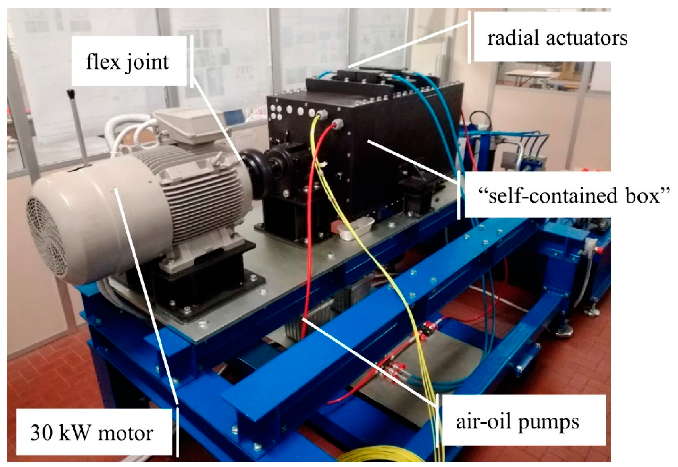
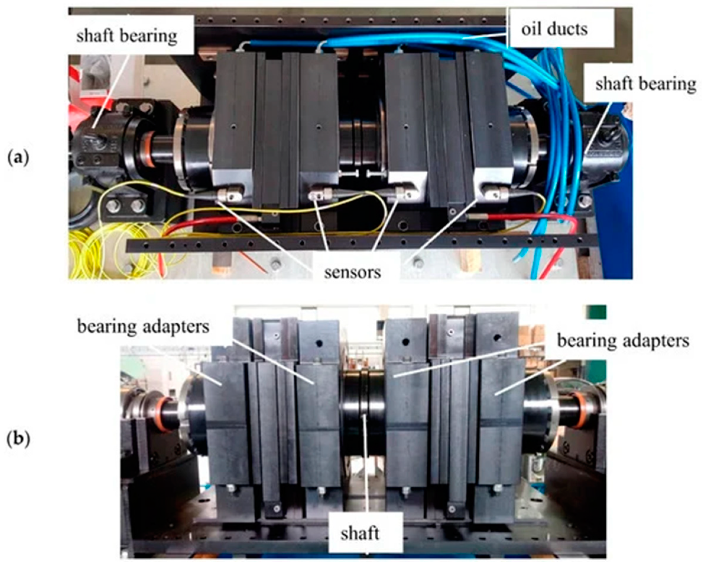
3.1. Test Rig Description

The test rig shown in Figure 1 is powered by a 30   kW three-phase motor by SIEMENS®, which is connected to the SIEMENS® G120_CU240E_2 INVERTER with a brake resistor that drives the shaft up to 195 Nm of the maximum torque at the rated spin speed of 1470 rpm. The speed and torque controls, managed by the inverter, can set the motor speed up to 2500 rpm. The “self-contained box” (Figure 2) is made of two housing blocks with oil lubrication and is equipped with up to four different roller bearings, whose reactions are directly balanced by the box. Hydraulic actuators on the upper panel of the box and between each pair of bearings allow the application of radial and axial static loads, respectively, up to 200   kN . The innovative design of the box makes it an isolated system with respect to all of the loads applied; in fact, radial and axial loads act only inside the box and are uncoupled with the outer part of the rotor system. The vibration signature is in the time and frequency domain as long as the operating temperature of each bearing under test can be measured through four SKF CMSS 2200 T sensors, which are mounted along the radial direction of the bearing-box adapters. Vibration signals are acquired through the LMS Scadas III Digital Acquisition system, equipped with four PQMAs (Programmable Quad Microphone Amplifiers). The main advantages of this test rig can be resumed as follows:
  • Independent radial and axial loads of up to 200 kN on each tested bearing;
  • Simultaneous testing of four bearings, which allows the self-balance of applied loads with minimal transmission to the platform;
  • High modularity, which enables testing on different sized bearings up to 420 mm of the outer diameter;
  • Direct measure of friction torque of tested bearings;
  • Main bearings are immune to the loads acting on the test bearings.

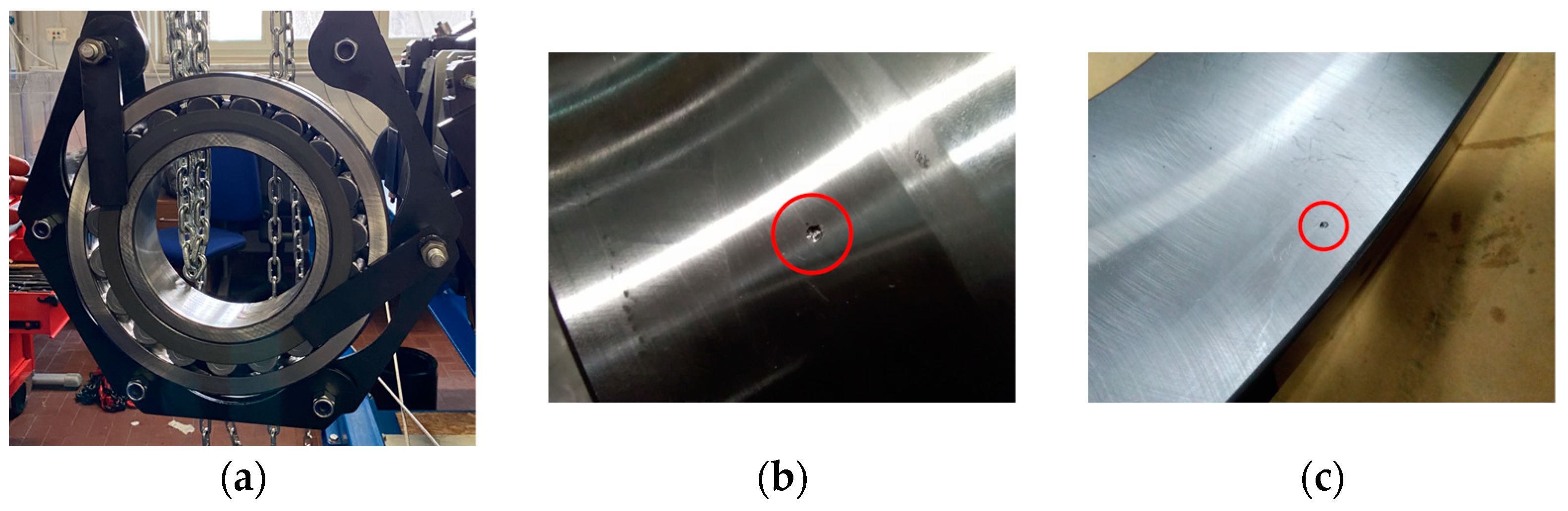
3.2. Vibration Dataset

The vibration signals coming from any bearing are always affected by the noise coming from the surrounding parts of the machine, which can make the recognition of defects and faults difficult [5]. In fact, those paths are usually complex and have non-stationary behaviour and the extraction of the required information could be hard [49]. For those reasons, a preliminary analysis of the vibration signature of the test rig in regular operating conditions is essential before the beginning of any condition monitoring activity [80].
In the experimental testing session carried out for the generation of the database of vibration data used in this work, four SKF spherical self-aligning bearings 22,240 CCK/W33 with a tapered bore and a 360   mm outer diameter were mounted inside the test rig. The vibration signals were acquired through the sensors and the DAQ system and were digitally sampled at f s = 20,480   Hz with AC coupling, which was used to remove the offset DC component of the voltage that was used to energise the piezoelectric accelerometers from the acquisition. A sixth-order Butterworth filter with a 10,200   Hz cut-off frequency was initially applied to the acquired signals and some digital filters were then designed for the elimination of the mechanical and electromagnetic noise to improve the signal-to-noise ratio (SNR).
Experimental data were obtained for three radial load cases over ten different rotational speeds and three defect conditions. The rotational speed refers to the three-phase motor synchronous velocity. Point defects were made by removing a circular portion of the material with a diameter of 2   mm and a depth of 0.5   mm from the raceways and only a single defect was present at a time in the bearing. The inner race (IR) and the outer race (OR) defects are shown in Figure 3, whereas Table 1 shows the operating conditions for the tests. Each recorded vibration path is 60   s long and the whole database consists of 90 vibration paths, labelled depending on the defect condition of the tested bearing.

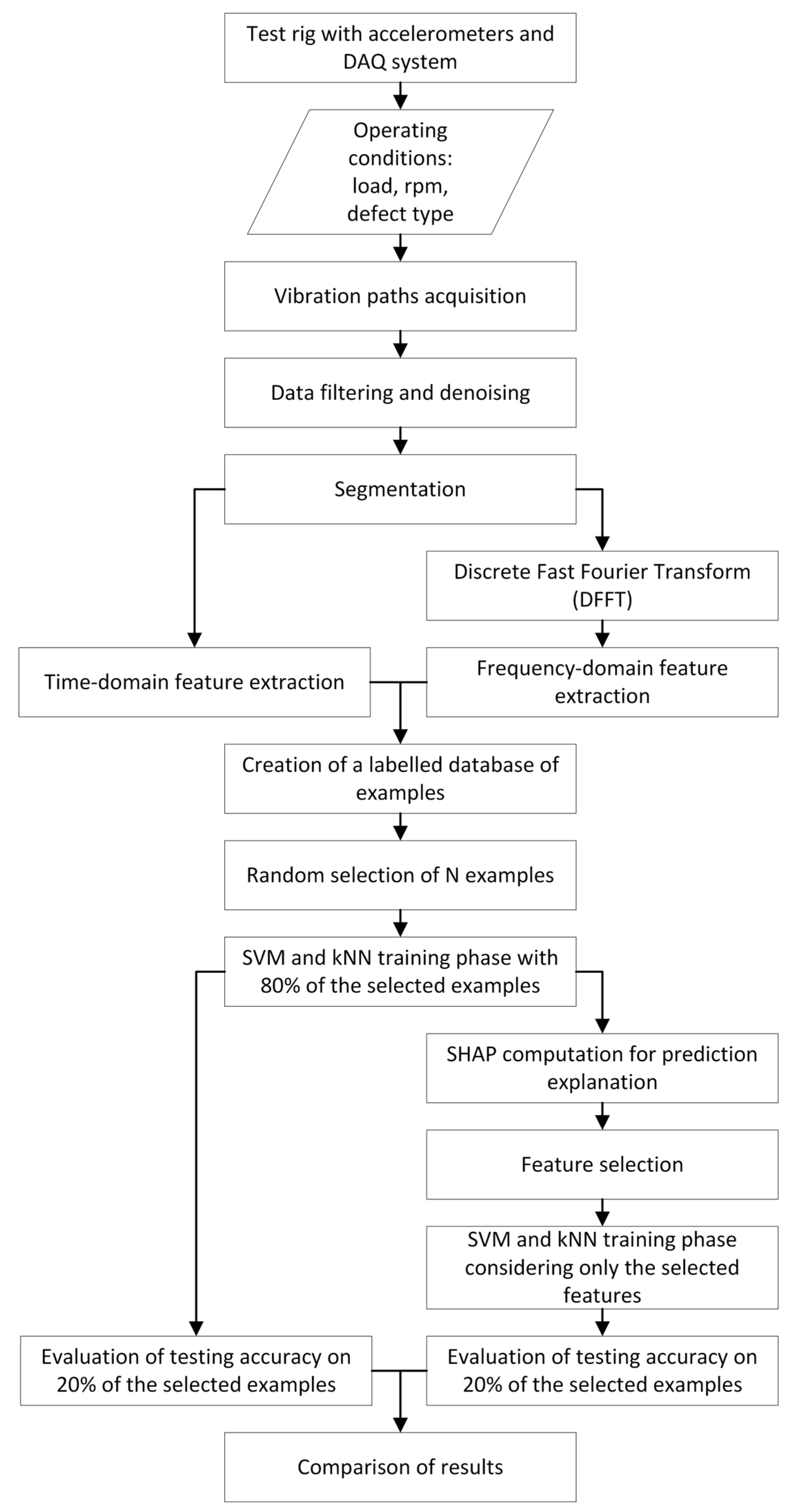
4. SHAP Analysis for Industrial Bearings

In this paragraph the proposed methodology for feature selection through the SHAP analysis is presented, and the results obtained in the above-mentioned experimental database are reported. All the computations were carried out using Matlab® and Python environments. These are the main steps of our method:
  • Vibration database acquisition and data pre-processing;
  • Feature extraction and creation of a database of the labelled samples;
  • Training of AI algorithms;
  • Shapley values computation and feature selection.
Figure 4 resumes the most important phases and operations performed in this work.

4.1. Features Extraction and Labelling of Vibration Samples

The extraction of the most relevant features from the data gathered during the collecting phase is the step following the data acquisition for the setup of the ML models. This stage is aimed at the identification and computation of representative features from the recorded data using a time-domain statistical analysis and a Fourier spectral analysis [95].
These characteristics can highlight the presence of defects, but they can also contain irrelevant information that can influence the performance of the classifier [96].
The features used in this work belong to the time and the frequency domain. The time-domain signal usually changes in its amplitude and distribution when a defect is present in one of the elements of the bearing since it induces some characteristics vibration impulses. For example, the mean, root mean square, and impulse factor reflect the vibration amplitude and energy, while the standard deviation, crest factor, kurtosis, and shape factor can be used to describe the time series distribution [97,98]. The frequency-domain parameters can add some information, which is not present in the time-domain. They can be extracted after the computation of the frequency-domain signal through the Discrete Fast Fourier Transform (DFFT) [99]. Commonly used frequency-domain features include the mean frequency, which represents the vibration energy, frequency centre, and root mean square frequency, which shows the position shift of the main excited frequencies and the standard deviation frequency that describes the degree of convergence of the spectrum power [100].
In this work, prior to the feature extraction, the vibration paths were segmented into 400   ms long intervals to achieve more examples for the training phase of the AI algorithms. From each segment, twenty-three features, taken from Lei et al. [101,102], were extracted and they are reported in Table 2. The first eleven parameters belong to the time-domain, whereas the others belong to the frequency domain: x i is the i-th acceleration sample, N is the number of data points in the time segment, s k is the k-th spectrum amplitude, K is the number of spectrum lines, and f k is the frequency value of the k-th spectrum line. After the feature extraction activity, a sample with twenty-three features and a label depending on the defect condition was generated from each segment. Therefore, a wide database of labelled samples was setup for the subsequent training phase.

4.2. Training of AI Algortihms

ML algorithms such as the SVM and kNN have been among the most used theories since the introduction of IFD [30]. For that reason, they were chosen for the analysis made in this work. Both the algorithms are characterised by some parameters that must be tuned to achieve their best performance.
As said previously, the goal of the SVM algorithm is the identification of the optimal hyperplane that maximises the margin of the training data and therefore, the distance between the nearest points of each class. The parameters that were tuned are the following:
  • The kernel function that defines the function of the hyperplane used to separate data;
  • C, called the regularisation term, which is the penalty parameter of the error term and controls the tradeoff between a smooth decision boundary and classifying the training points correctly;
  • γ, which influences the number of nearby points used for the calculation of the separating hyperplane using the radial basis function (RBF) kernel.
Regarding the kNN algorithm, the main tuneable parameter is the number of neighbours k , which represents the number of the closest training examples that are considered for the classification of a new point. The training of the algorithms and optimisation of the tuneable parameters were carried out through the Python function GridSearchCV, using a 5-fold cross-validation, and the main parameters of the optimised algorithms are resumed in Table 3, where d is the number of features and σ X is the variance of the feature database. Before the training phase, N = 2000 samples were randomly selected from the original database and then split into two sets with a ratio 80 / 20 : the bigger dataset was used for the training phase itself, while the other one was used for the evaluation of the algorithms testing accuracy.

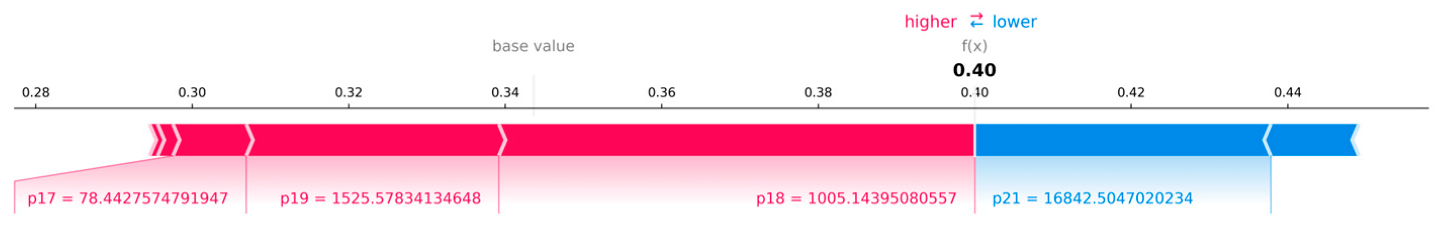
4.3. Shapley Values Computation and Features Selection

When a trained model provides an outcome for a regression or classification task, we may want to analyse its behaviour with respect to the inputs and outputs in an easy and understandable way, since the accuracy does not give a complete and exhaustive description of the performance [34]. For example, the decision process of non-linear and complex models is often difficult to be understood. To evaluate the performance of the proposed AI algorithms and the contribution of each feature to the outcome of the classification problem, three stages were implemented in this study:
  • Computation of Shapley values;
  • Feature selection;
  • Accuracy evaluation.
The SHAP values can be analysed from two points of view: they are the expression of the contribution of each feature to the outcome of a single classification outcome or, on the other side, we can study how these values are attributed globally for each feature.
The SHAP values computed on each point explain how each feature contributed to the model classification prediction, by modifying the base value, which is the mean prediction of the model trained on the specific set of data used in the training phase. Figure 5 shows how each feature contributes to the change of the base value towards higher or lower values. The base value of each class is the probability that a sample is classified into that class, independent of the values of its features. Therefore, it is highly linked to the probability distribution of the training examples among the classes. On the contrary, the final value of the prediction represents the probability of the point under investigation to be classified in that specific class and it is the result of the feature contribution: if the computed value is one, the predicted probability of a specific fault by the model is 100%. Thus, the outcome of the classification would be the class with the highest probability. In this specific case the base value is around 0.34. This is plausible because, since the training examples were taken randomly from the database, the distribution among the selected examples of each of the three defect classes should be around 33%. Then, the base value is modified by each feature, depending on its value. The amounts of contribution of each feature is represented by the Shapley value and is displayed by an arrow that pushes to increase or decrease the prediction. During the training phase, the SHAP algorithm learns a threshold value for each feature that is related to each different class to determine if that feature, depending on its value, will have a positive or negative effect towards the prediction and the magnitude of the contribution. For example, a certain feature can have a positive effect on a class and a negative effect on the others. From Figure 5 It can be seen that p 17 , p 18 , and p 19 (red arrows) are the most important features in increasing the probability of this example to be classified in that class, whereas p 21 (blue arrow) is the most influent in decreasing the base value. Features can have a positive or a negative contribution depending on their value, which is related to the threshold value computed in the training phase of the algorithm. The final value, which is 0.40, tells that the sample under investigation has a 40% probability to be classified in this defect class.
Then, if this computation is replicated for the entire dataset, it is possible to analyse how the SHAP values are attributed to features globally. The computation of the Shapley values was performed using the “shapley” library in Python on both the optimised algorithms trained on the previously cited training set with N t r a i n = 1600 examples. The Shapley values were computed using the first 500 samples of the training set. Only the ten most important features, selected depending on the overall absolute value of their Shapley values, were plotted for each one of the three classes of defect.

5. Results and Discussion

Figure 6 shows the SHAP values obtained for different damage classes when the SVM and the kNN algorithms are applied; similarly, Figure 7 shows the mean SHAP values for the features. The plots of Figure 6 present the features sorted along the y -axis depending on their impact on the output, but they also report the SHAP values of every feature computed on each example of the dataset. As stated in Shapley [92], for the feature with the highest importance, their SHAP values span over a greater range than the rest. Points are also coloured depending on their value. In this way, it is easy to figure out when a feature has a high or low impact on the output and when it contributes to increasing or decreasing the base probability value of each class. Interestingly, the impact on model outputs given by the analysed features is similar in both the ML models. For instance, high values of the feature p 6 have a positive impact for the class zero and the class one, whereas high values of the feature p 6 have a negative impact for the class two, which is the outer race damage. This means that signals characterised by high values of p 6 are very unlikely to belong to bearings that are damaged on the outer race. For some features, such as p 19 and p 3 , a similar attitude is detectable for both the models.
Figure 7 reports the SHAP values of the ten most important features, which are sorted depending on their average impact on predictions for the three different defect conditions. As it can be seen from those plots, p 6 , which is the skewness parameter, is by far the most important feature for the classification of the bearing defect condition for both the SVM and kNN algorithms. Skewness is the ratio of the average deviation from the mean cubed divided by the standard deviation cubed; for a random variable with normal distribution, the skewness is zero. Higher values of skewness discriminate between an outer race defect and the other two defect conditions. For classes zero and two, the skewness has a much higher mean SHAP value than the other features. Other important features for both the algorithms that belong to the time-domain are p 3 , the squared mean root of absolute values (SMRA), which is determinant in the recognition of the defect-free class, and p 10 , the shape factor, which is a parameter dependent on the signal shape that seems to be important in the discrimination between the inner and the outer race defect, especially for the SVM. The skewness and shape factor were also found to be relevant features in other works, such as the one from Hui et al. [41]. The last two relevant parameters that are in common with both the algorithms are p 18 and p 19 : the former, which is the root mean square frequency, is nearly the most important feature for class one, while the latter has a greater impact on kNN.
After the SHAP analysis was carried out, the four most important features of each class were selected for the SVM and kNN algorithms. Table 4 reports all the selected features for each algorithm. In kNN, only five features appear in the top four places of the three different defect-related classes, while the most relevant features related to the SVM are nine. Therefore, the kNN model is explained by fewer parameters, with respect to the SVM. The influence of the feature selection activity was evaluated by comparing the accuracy of the algorithm trained considering all the twenty-three features, or only the features in Table 4 that are in common to both the SVM and kNN, which are p 3 , p 6 , p 10 , p 18 , and p 19 . For this task, 100 different datasets containing N = 2000 randomly selected samples from the original database were used. Each dataset was split into two subsets with a ratio 80 / 20 : the former was used for the training phase, while the latter was used for the computation of the testing accuracy. The accuracy of the algorithms in both the considered cases and for each set of data was recorded and the mean accuracy was computed to analyse the overall impact of the feature selection activity. The results are reported in Figure 8.
Thus, with the help of the insights provided by the SHAP analysis, the number of relevant features could be reduced with proper justification, making the ML models more robust and easily explainable in terms of feature importance for the outcome of the model. As it can be seen from Figure 8a, the accuracy for the SVM is only 1% worse, as if it has been trained considering all the features, whereas Figure 8b shows that the kNN algorithm performs better only if the most important features are considered. This was expected, because, as cited previously, this kind of algorithm suffers from feature redundancy. Then, diagnosis accuracies are not significantly affected by the selection of only five features out of twenty-three, as long as the SHAP values are employed to select the relevant features by means of model explanations.

6. Conclusions

This study aimed at investigating the capabilities of SHAP for explaining machine learning models in the intelligent fault diagnosis of industrial bearings. Additionally, this results in identifying the most relevant features for diagnosis. The explanations of the diagnosis outcomes were provided for the SVM and kNN models. The authors investigated the case provided by the test rig for industrial bearings available at the Mechanical Engineering Laboratory of Politecnico di Torino. The conclusions are as follows:
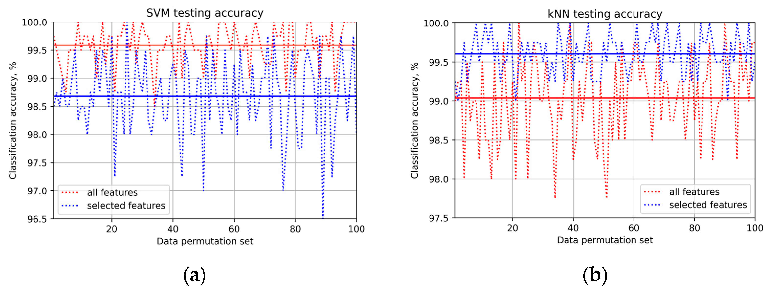
  • The SVM and the kNN models are able to achieve diagnosis accuracies higher than 98.5% for medium-sized industrial bearings;
  • The SHAP values are effective for interpreting machine learning models that are aimed at industrial condition monitoring;
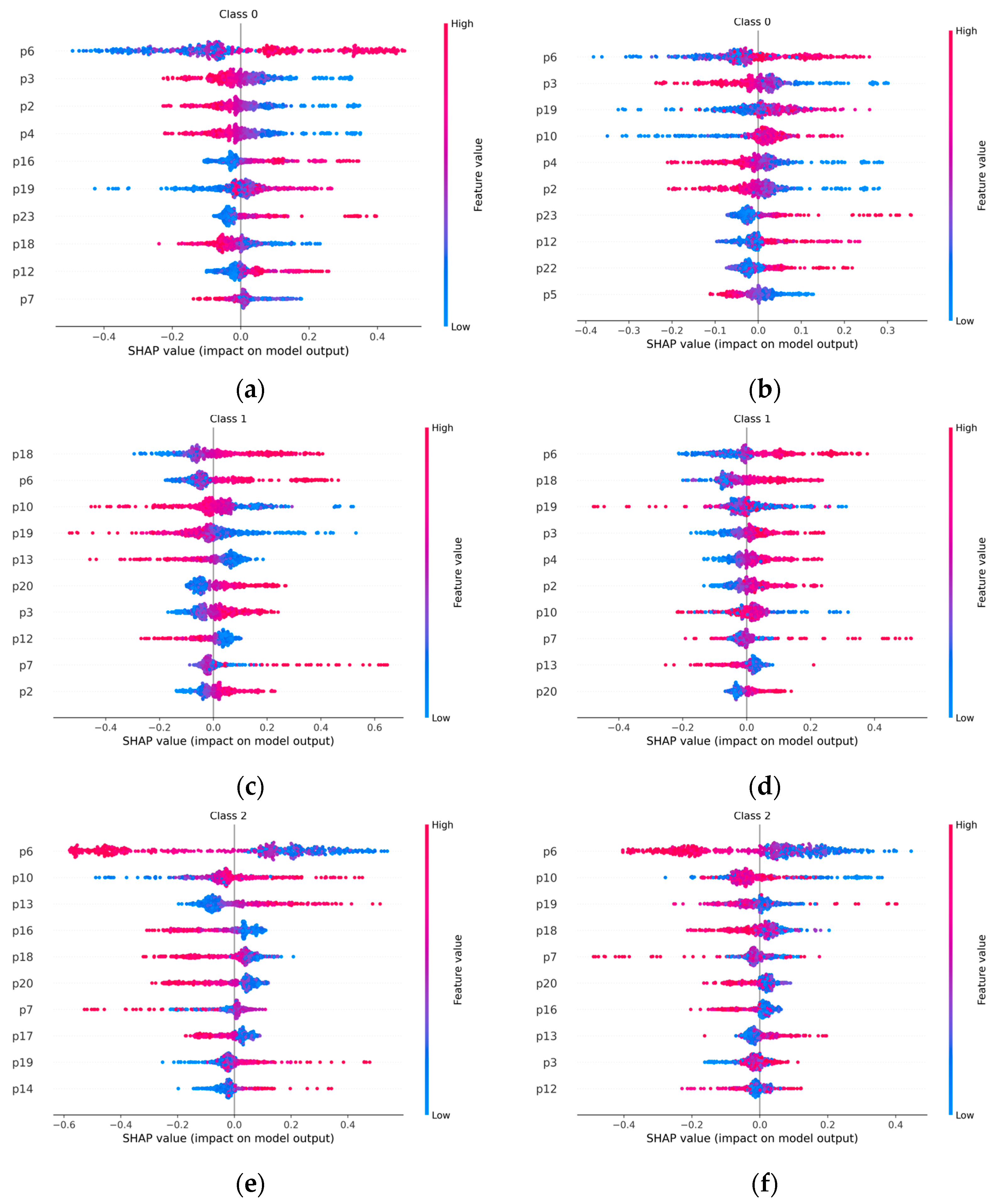
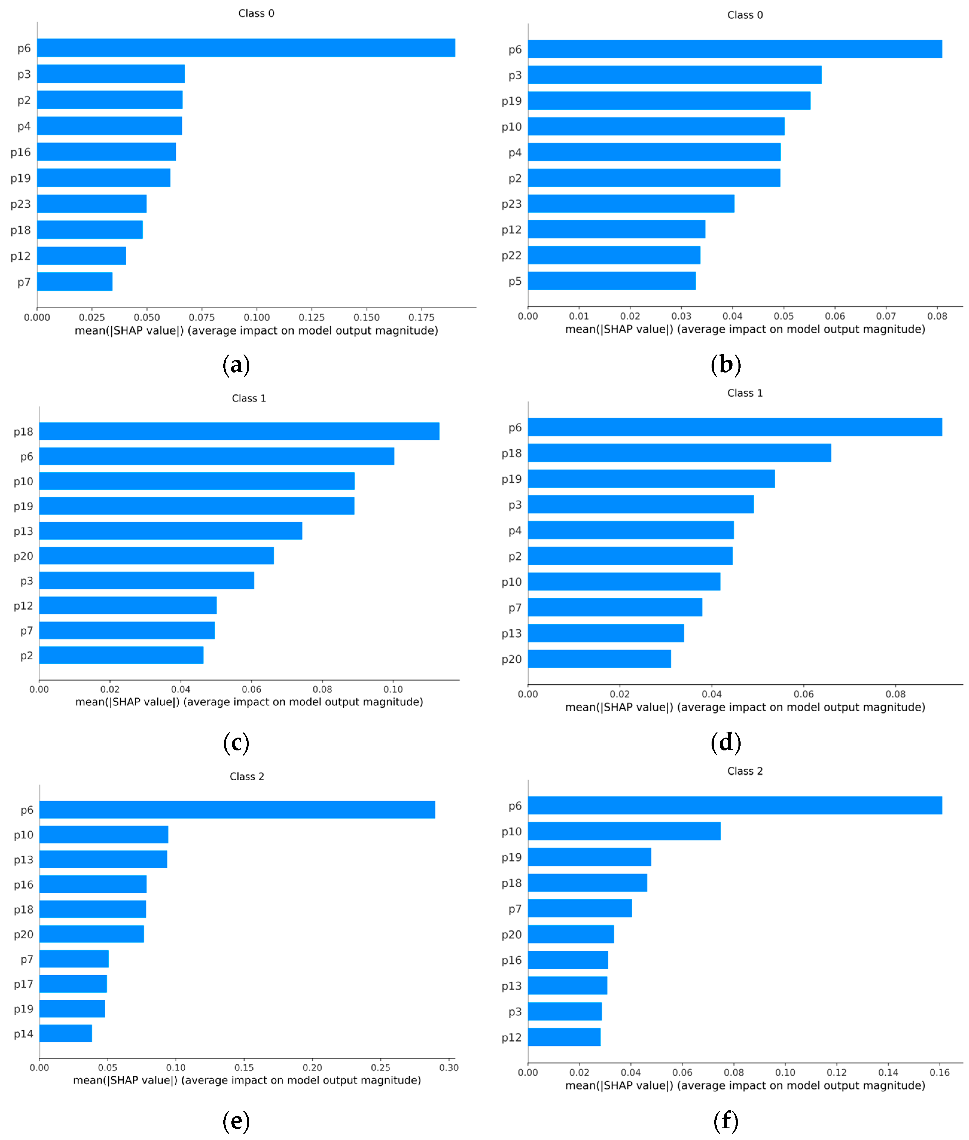
  • The SHAP analysis is employed to show that four features out of twenty-three are really important to achieve good diagnosis accuracies;
  • The skewness and the shape factor of the vibration signals have the greatest impact on the outcomes of machine learning diagnosis models.
The generalisability of these results is subjected to certain limitations. For instance, the choice of the diagnosis model could influence the explainability. Then, future works will provide explanations for different ML models, and the results will be compared with those of this study. Especially, research will be focused on deep learning, which is the most used in IFD nowadays, because it allows the automatic learning of fault features from the collected data instead of the artificial feature extraction, attempting to provide end-to-end diagnosis models when handling increasingly grown data and connecting the raw monitoring data to their corresponding health states of machines, which will further release the contribution of human labour [30,103]. Another field of investigation will be the effect of the feature selection through the SHAP analysis on the computation time. We noticed a little improvement in the computation time between the ML model trained with all the features and those trained only with the selected ones, but since the SHAP analysis is computationally very expensive, an overall time saving could not be achieved. However, as it is reported in the literature [75,76], ML models involving deep learning techniques could take advantage of the feature selection through the SHAP method in terms of the computation time, and, therefore, it will be the subject of our future study. Additionally, the feature selection capabilities should be assessed on a general level, and we will mainly focus on feature selection capabilities besides explainability, by providing proper comparisons with the common techniques targeted in this task.

Author Contributions

Conceptualisation, E.B., L.C., C.D., and L.G.D.M.; methodology, L.C. and L.G.D.M.; software, L.C.; investigation, L.C. and L.G.D.M.; data curation, L.G.D.M.; writing—original draft preparation, L.C. and L.G.D.M.; writing—review and editing, E.B. and C.D.; project administration, E.B. and C.D.; supervision, E.B. and C.D. All authors have read and agreed to the published version of the manuscript.

Funding

This research received no external funding.

Institutional Review Board Statement

Not applicable.

Informed Consent Statement

Not applicable.

Data Availability Statement

Data are not available due to privacy reasons.

Conflicts of Interest

The authors declare no conflict of interest.

References

  1. Lei, Y.; He, Z.; Zi, Y. A New Approach to Intelligent Fault Diagnosis of Rotating Machinery. Expert Syst. Appl. 2008, 35, 1593–1600. [Google Scholar] [CrossRef]
  2. Gupta, P.K. Advanced Dynamics of Rolling Elements; Springer: New York, NY, USA, 1984; ISBN 978-1-4612-9767-3. [Google Scholar]
  3. Singh, S.; Howard, C.Q.; Hansen, C.H. An Extensive Review of Vibration Modelling of Rolling Element Bearings with Localised and Extended Defects. J. Sound Vib. 2015, 357, 300–330. [Google Scholar] [CrossRef]
  4. Yan, X.; Jia, M. A Novel Optimized SVM Classification Algorithm with Multi-Domain Feature and Its Application to Fault Diagnosis of Rolling Bearing. Neurocomputing 2018, 313, 47–64. [Google Scholar] [CrossRef]
  5. Hasan, M.J.; Sohaib, M.; Kim, J.-M. A Multitask-Aided Transfer Learning-Based Diagnostic Framework for Bearings under Inconsistent Working Conditions. Sensors 2020, 20, 7205. [Google Scholar] [CrossRef] [PubMed]
  6. Cui, L.; Huang, J.; Zhang, F. Quantitative and Localization Diagnosis of a Defective Ball Bearing Based on Vertical–Horizontal Synchronization Signal Analysis. IEEE Trans. Ind. Electron. 2017, 64, 8695–8706. [Google Scholar] [CrossRef]
  7. Tian, J.; Ai, Y.; Zhao, M.; Zhang, F.; Wang, Z.-J. Fault Diagnosis of Intershaft Bearings Using Fusion Information Exergy Distance Method. Shock. Vib. 2018, 2018, 7546128. [Google Scholar] [CrossRef]
  8. Rai, A.; Kim, J.-M. A Novel Health Indicator Based on the Lyapunov Exponent, a Probabilistic Self-Organizing Map, and the Gini-Simpson Index for Calculating the RUL of Bearings. Measurement 2020, 164, 108002. [Google Scholar] [CrossRef]
  9. Hasan, M.J.; Sohaib, M.; Kim, J.-M. An Explainable Ai-Based Fault Diagnosis Model for Bearings. Sensors 2021, 21, 4070. [Google Scholar] [CrossRef]
  10. Lacey, S.J. An Overview of Bearing Vibration Analysis. Maint. Asset Manag. 2008, 23, 32–42. [Google Scholar]
  11. Zheng, H.; Wang, R.; Yang, Y.; Li, Y.; Xu, M. Intelligent Fault Identification Based on Multisource Domain Generalization Towards Actual Diagnosis Scenario. IEEE Trans. Ind. Electron. 2020, 67, 1293–1304. [Google Scholar] [CrossRef]
  12. Oh, H.; Jung, J.H.; Jeon, B.C.; Youn, B.D. Scalable and Unsupervised Feature Engineering Using Vibration-Imaging and Deep Learning for Rotor System Diagnosis. IEEE Trans. Ind. Electron. 2018, 65, 3539–3549. [Google Scholar] [CrossRef]
  13. Brusa, E.; Bruzzone, F.; Delprete, C.; Di Maggio, L.G.; Rosso, C. Health Indicators Construction for Damage Level Assessment in Bearing Diagnostics: A Proposal of an Energetic Approach Based on Envelope Analysis. Appl. Sci. 2020, 10, 8131. [Google Scholar] [CrossRef]
  14. Delprete, C.; Brusa, E.; Rosso, C.; Bruzzone, F. Bearing Health Monitoring Based on the Orthogonal Empirical Mode Decomposition. Shock. Vib. 2020, 2020, 8761278. [Google Scholar] [CrossRef]
  15. Delprete, C.; Milanesio, M.; Rosso, C. Rolling Bearings Monitoring and Damage Detection Methodology. Appl. Mech. Mater. 2006, 3–4, 293–302. [Google Scholar] [CrossRef]
  16. Brusa, E.; Delprete, C.; Giorio, L. Smart Manufacturing in Rolling Process Based on Thermal Safety Monitoring by Fiber Optics Sensors Equipping Mill Bearings. Appl. Sci. 2022, 12, 4186. [Google Scholar] [CrossRef]
  17. Li, Y.; Miao, B.; Zhang, W.; Chen, P.; Liu, J.; Jiang, X. Refined Composite Multiscale Fuzzy Entropy: Localized Defect Detection of Rolling Element Bearing. J. Mech. Sci. Technol. 2019, 33, 109–120. [Google Scholar] [CrossRef]
  18. Zhu, X.; Xiong, J.; Liang, Q. Fault Diagnosis of Rotation Machinery Based on Support Vector Machine Optimized by Quantum Genetic Algorithm. IEEE Access 2018, 6, 33583–33588. [Google Scholar] [CrossRef]
  19. Kang, M.; Kim, J.; Kim, J.-M.; Tan, A.C.C.; Kim, E.Y.; Choi, B.-K. Reliable Fault Diagnosis for Low-Speed Bearings Using Individually Trained Support Vector Machines With Kernel Discriminative Feature Analysis. IEEE Trans. Power Electron. 2015, 30, 2786–2797. [Google Scholar] [CrossRef]
  20. Widodo, A.; Kim, E.Y.; Son, J.-D.; Yang, B.-S.; Tan, A.C.C.; Gu, D.-S.; Choi, B.-K.; Mathew, J. Fault Diagnosis of Low Speed Bearing Based on Relevance Vector Machine and Support Vector Machine. Expert Syst. Appl. 2009, 36, 7252–7261. [Google Scholar] [CrossRef]
  21. Brusa, E.; Delprete, C.; Di Maggio, L.G. Eigen-Spectrograms: An Interpretable Feature Space for Bearing Fault Diagnosis Based on Artificial Intelligence and Image Processing. Mech. Adv. Mater. Struct. 2022, 1–13. [Google Scholar] [CrossRef]
  22. He, D.; Li, R.; Zhu, J. Plastic Bearing Fault Diagnosis Based on a Two-Step Data Mining Approach. IEEE Trans. Ind. Electron. 2013, 60, 3429–3440. [Google Scholar] [CrossRef]
  23. Safizadeh, M.S.; Latifi, S.K. Using Multi-Sensor Data Fusion for Vibration Fault Diagnosis of Rolling Element Bearings by Accelerometer and Load Cell. Inf. Fusion 2014, 18, 1–8. [Google Scholar] [CrossRef]
  24. Yang, D.-M.; Stronach, A.F.; Macconnell, P.; Penman, J. THIRD-ORDER SPECTRAL TECHNIQUES FOR THE DIAGNOSIS OF MOTOR BEARING CONDITION USING ARTIFICIAL NEURAL NETWORKS. Mech. Syst. Signal Process. 2002, 16, 391–411. [Google Scholar] [CrossRef]
  25. Zarei, J.; Tajeddini, M.A.; Karimi, H.R. Vibration Analysis for Bearing Fault Detection and Classification Using an Intelligent Filter. Mechatronics 2014, 24, 151–157. [Google Scholar] [CrossRef]
  26. He, X.; Wang, D.; Li, Y.; Zhou, C. A Novel Bearing Fault Diagnosis Method Based on Gaussian Restricted Boltzmann Machine. Math. Probl. Eng. 2016, 2016, 2957083. [Google Scholar] [CrossRef]
  27. Guo, S.; Yang, T.; Gao, W.; Zhang, C. A Novel Fault Diagnosis Method for Rotating Machinery Based on a Convolutional Neural Network. Sensors 2018, 18, 1429. [Google Scholar] [CrossRef]
  28. Brusa, E.; Delprete, C.; Di Maggio, L.G. Deep Transfer Learning for Machine Diagnosis: From Sound and Music Recognition to Bearing Fault Detection. Appl. Sci. 2021, 11, 11663. [Google Scholar] [CrossRef]
  29. Di Maggio, L.G. Intelligent Fault Diagnosis of Industrial Bearings Using Transfer Learning and CNNs Pre-Trained for Audio Classification. Sensors 2022, 23, 211. [Google Scholar] [CrossRef]
  30. Lei, Y.; Yang, B.; Jiang, X.; Jia, F.; Li, N.; Nandi, A.K. Applications of Machine Learning to Machine Fault Diagnosis: A Review and Roadmap. Mech. Syst. Signal Process. 2020, 138, 106587. [Google Scholar] [CrossRef]
  31. Islam, M.R.; Islam, M.M.M.; Kim, J.-M. Feature Selection Techniques for Increasing Reliability of Fault Diagnosis of Bearings. In Proceedings of the 2016 9th International Conference on Electrical and Computer Engineering (ICECE), Dhaka, Bangladesh, 20–22 December 2016; pp. 396–399. [Google Scholar]
  32. Roelofs, R.; Shankar, V.; Recht, B.; Fridovich-Keil, S.; Hardt, M.; Miller, J.; Schmidt, L. A Meta-Analysis of Overfitting in Machine Learning. In Proceedings of the Advances in Neural Information Processing Systems; Curran Associates, Inc.: Vancouver, BC, Canada, 2019; Volume 32. [Google Scholar]
  33. Yassine, A.; Mohamed, C.; Zinedine, A. Feature Selection Based on Pairwise Evalution. In Proceedings of the 2017 Intelligent Systems and Computer Vision (ISCV), Fez, Morocco, 17–19 April 2017; pp. 1–6. [Google Scholar]
  34. Vega García, M.; Aznarte, J.L. Shapley Additive Explanations for NO2 Forecasting. Ecol. Inform. 2020, 56, 101039. [Google Scholar] [CrossRef]
  35. Kononenko, I. Estimating Attributes: Analysis and Extensions of RELIEF. In Proceedings of the Machine Learning: ECML-94; Bergadano, F., De Raedt, L., Eds.; Springer: Berlin/Heidelberg, Germany, 1994; pp. 171–182. [Google Scholar]
  36. Hall, M.A.; Smith, L.A. Practical Feature Subset Selection for Machine Learning. In Proceedings of the 21st Australasian Computer Science Conference ACSC’98, Perth, Australia, 6 February 1998; Volume 20, pp. 181–191. [Google Scholar]
  37. Peng, H.; Long, F.; Ding, C. Feature Selection Based on Mutual Information Criteria of Max-Dependency, Max-Relevance, and Min-Redundancy. IEEE Trans. Pattern Anal. Mach. Intell. 2005, 27, 1226–1238. [Google Scholar] [CrossRef]
  38. Bishop, C.M. Neural Networks for Pattern Recognition; Oxford University Press: Oxford, UK, 1995. [Google Scholar]
  39. Yang, B.S.; Han, T.; An, J.L. ART–KOHONEN Neural Network for Fault Diagnosis of Rotating Machinery. Mech. Syst. Signal Process. 2004, 18, 645–657. [Google Scholar] [CrossRef]
  40. Landau, S.; Leese, M.; Stahl, D.; Everitt, B.S. Cluster Analysis; John Wiley & Sons: Hoboken, NJ, USA, 2011; ISBN 978-0-470-97844-3. [Google Scholar]
  41. Hui, K.H.; Ooi, C.; Lim, M.; Leong, M.; Al-Obaidi, S. An Improved Wrapper-Based Feature Selection Method for Machinery Fault Diagnosis. PLoS ONE 2017, 12, e0189143. [Google Scholar] [CrossRef] [PubMed]
  42. Tibshirani, R.; Saunders, M.; Rosset, S.; Zhu, J.; Knight, K. Sparsity and Smoothness via the Fused Lasso. J. R. Stat. Soc. Ser. B 2005, 67, 91–108. [Google Scholar] [CrossRef]
  43. Tikhonov, A.N.; Goncharsky, A.V.; Stepanov, V.V.; Yagola, A.G. Numerical Methods for the Solution of Ill-Posed Problems; Springer: Dordrecht, The Netherlands, 1995; ISBN 978-90-481-4583-6. [Google Scholar]
  44. Qin, S.J. Survey on Data-Driven Industrial Process Monitoring and Diagnosis. Annu. Rev. Control. 2012, 36, 220–234. [Google Scholar] [CrossRef]
  45. Yadav, A.; Swetapadma, A. A Novel Transmission Line Relaying Scheme for Fault Detection and Classification Using Wavelet Transform and Linear Discriminant Analysis. Ain Shams Eng. J. 2015, 6, 199–209. [Google Scholar] [CrossRef]
  46. MacGregor, J.F.; Jaeckle, C.; Kiparissides, C.; Koutoudi, M. Process Monitoring and Diagnosis by Multiblock PLS Methods. AIChE J. 1994, 40, 826–838. [Google Scholar] [CrossRef]
  47. Lundberg, S.M.; Lee, S.-I. A Unified Approach to Interpreting Model Predictions. In Proceedings of the Advances in Neural Information Processing Systems; Guyon, I., Luxburg, U.V., Bengio, S., Wallach, H., Fergus, R., Vishwanathan, S., Garnett, R., Eds.; Curran Associates, Inc.: Long Beach, CA, USA, 2017; Volume 30. [Google Scholar]
  48. Choi, S.H.; Lee, J.M. Explainable Fault Diagnosis Model Using Stacked Autoencoder and Kernel SHAP. In Proceedings of the 2022 IEEE International Symposium on Advanced Control of Industrial Processes (AdCONIP), Vancouver, BC, Canada, 7–9 August 2022; pp. 182–187. [Google Scholar]
  49. Brito, L.C.; Susto, G.A.; Brito, J.N.; Duarte, M.A.V. An Explainable Artificial Intelligence Approach for Unsupervised Fault Detection and Diagnosis in Rotating Machinery. Mech. Syst. Signal Process. 2022, 163, 108105. [Google Scholar] [CrossRef]
  50. Adadi, A.; Berrada, M. Peeking Inside the Black-Box: A Survey on Explainable Artificial Intelligence (XAI). IEEE Access 2018, 6, 52138–52160. [Google Scholar] [CrossRef]
  51. Doran, D.; Schulz, S.; Besold, T.R. What Does Explainable AI Really Mean? A New Conceptualization of Perspectives. arXiv 2017. [Google Scholar] [CrossRef]
  52. Song, E.; Nelson, B.L.; Staum, J. Shapley Effects for Global Sensitivity Analysis: Theory and Computation. SIAM/ASA J. Uncertain. Quantif. 2016, 4, 1060–1083. [Google Scholar] [CrossRef] [Green Version]
  53. Aas, K.; Jullum, M.; Løland, A. Explaining Individual Predictions When Features Are Dependent: More Accurate Approximations to Shapley Values. Artif. Intell. 2021, 298, 103502. [Google Scholar] [CrossRef]
  54. Lundberg, S.; Erion, G.; Chen, H.; DeGrave, A.; Prutkin, J.; Nair, B.; Katz, R.; Himmelfarb, J.; Bansal, N.; Lee, S.-I. Explainable AI for Trees: From Local Explanations to Global Understanding. arXiv 2019, arXiv:1905.04610. [Google Scholar] [CrossRef] [PubMed]
  55. Štrumbelj, E.; Kononenko, I. Explaining Prediction Models and Individual Predictions with Feature Contributions. Knowl. Inf. Syst. 2014, 41, 647–665. [Google Scholar] [CrossRef]
  56. Redelmeier, A.; Jullum, M.; Aas, K. Explaining Predictive Models with Mixed Features Using Shapley Values and Conditional Inference Trees. In Machine Learning and Knowledge Extraction; Lecture Notes in Computer Science; Holzinger, A., Kieseberg, P., Tjoa, A.M., Weippl, E., Eds.; Springer International Publishing: Cham, Oslo, Norway, 2020; Volume 12279, pp. 117–137. ISBN 978-3-030-57320-1. [Google Scholar]
  57. Moehle, N.; Boyd, S.; Ang, A. Portfolio Performance Attribution via Shapley Value. arXiv 2021, arXiv:2102.05799. [Google Scholar]
  58. Fryer, D.; Strümke, I.; Nguyen, H. Shapley Values for Feature Selection: The Good, the Bad, and the Axioms. IEEE Access 2021, 9, 144352–144360. [Google Scholar] [CrossRef]
  59. Strumbelj, E.; Kononenko, I. An Efficient Explanation of Individual Classifications Using Game Theory. J. Mach. Learn. Res. 2010, 11, 1–18. [Google Scholar]
  60. Banerjee, T.; Paul, A.; Srikanth, V.; Strümke, I. Causal Connections between Socioeconomic Disparities and COVID-19 in the USA. Sci. Rep. 2022, 12, 15827. [Google Scholar] [CrossRef]
  61. Rohmer, J.; Thieblemont, R.; Le Cozannet, G.; Goelzer, H.; Durand, G. Improving Interpretation of Sea-Level Projections through a Machine-Learning-Based Local Explanation Approach. Cryosphere 2022, 16, 4637–4657. [Google Scholar] [CrossRef]
  62. Watson, D.S. Interpretable Machine Learning for Genomics. Hum. Genet. 2022, 141, 1499–1513. [Google Scholar] [CrossRef]
  63. Midtfjord, A.D.; Bin, R.D.; Huseby, A.B. A Decision Support System for Safer Airplane Landings: Predicting Runway Conditions Using XGBoost and Explainable AI. Cold Reg. Sci. Technol. 2022, 199, 103556. [Google Scholar] [CrossRef]
  64. Dong, H.; Sun, J.; Sun, X. A Multi-Objective Multi-Label Feature Selection Algorithm Based on Shapley Value. Entropy 2021, 23, 1094. [Google Scholar] [CrossRef]
  65. Goštautaitė, D.; Sakalauskas, L. Multi-Label Classification and Explanation Methods for Students’ Learning Style Prediction and Interpretation. Appl. Sci. 2022, 12, 5396. [Google Scholar] [CrossRef]
  66. Chen, Y.; Aleman, D.M.; Purdie, T.G.; McIntosh, C. Understanding Machine Learning Classifier Decisions in Automated Radiotherapy Quality Assurance. Phys. Med. Biol. 2022, 67, 025001. [Google Scholar] [CrossRef]
  67. Oh, A.R.; Park, J.; Lee, J.-H.; Kim, H.; Yang, K.; Choi, J.-H.; Ahn, J.; Sung, J.D.; Lee, S.-H. Association Between Perioperative Adverse Cardiac Events and Mortality During One-Year Follow-Up After Noncardiac Surgery. J. Am. Heart Assoc. 2022, 11, e024325. [Google Scholar] [CrossRef]
  68. Akimoto, S.; Lebreton, P.; Takahashi, S.; Yamagishi, K. Quantitative Causality Analysis of Viewing Abandonment Reasons Using Shapley Value. In Proceedings of the 2022 IEEE 24th International Workshop on Multimedia Signal Processing (MMSP), Shanghai, China, 26–28 September 2022; pp. 01–06. [Google Scholar]
  69. Li, L.; Wu, X.; Kong, M.; Zhou, D.; Tao, X. Towards the Quantitative Interpretability Analysis of Citizens Happiness Prediction. In Proceedings of the 39th International Joint Conference on Artificial Intelligence (IJCAI-ECAI 2022), Vienna, Austria, 23–29 July 2022; Volume 6, pp. 5094–5100. [Google Scholar]
  70. Sun, Q.; Sun, J.; Guo, K.; Liu, J. Investigation on Mechanical Properties and Energy Absorption Capabilities of AlSi10Mg Triply Periodic Minimal Surface Sheet Structures Fabricated via Selective Laser Melting. J. Mater. Eng. Perform. 2022, 31, 9110–9121. [Google Scholar] [CrossRef]
  71. Remman, S.B.; Strumke, I.; Lekkas, A.M. Causal versus Marginal Shapley Values for Robotic Lever Manipulation Controlled Using Deep Reinforcement Learning. In Proceedings of the 2022 American Control Conference (ACC), Atlanta, GA, USA, 8–10 June 2022; Volume 2022, pp. 2683–2690. [Google Scholar]
  72. Cohen, S.; Ruppin, E.; Dror, G. Feature Selection Based on the Shapley Value. In Proceedings of the 19th International Joint Conference on Artificial Intelligence, Montreal, QC, Canada, 19–27 August 2005; Cohen, S., Ruppin, E., Dror, G., Eds.; Morgan Kaufmann Publishers Inc.: San Francisco, CA, USA, 2005; pp. 665–670. [Google Scholar]
  73. Marcílio, W.E.; Eler, D.M. From Explanations to Feature Selection: Assessing SHAP Values as Feature Selection Mechanism. In Proceedings of the 2020 33rd SIBGRAPI Conference on Graphics, Patterns and Images (SIBGRAPI), Porto de Galinhas, Brazil, 7–10 November 2020; pp. 340–347. [Google Scholar]
  74. Zacharias, J.; von Zahn, M.; Chen, J.; Hinz, O. Designing a Feature Selection Method Based on Explainable Artificial Intelligence. Electron. Mark. 2022, 32, 2159–2184. [Google Scholar] [CrossRef]
  75. Guha, R.; Khan, A.H.; Singh, P.K.; Sarkar, R.; Bhattacharjee, D. CGA: A New Feature Selection Model for Visual Human Action Recognition. Neural Comput. Applic 2021, 33, 5267–5286. [Google Scholar] [CrossRef]
  76. Jothi, N.; Husain, W.; Rashid, N.A. Predicting Generalized Anxiety Disorder among Women Using Shapley Value. J. Infect. Public Health 2021, 14, 103–108. [Google Scholar] [CrossRef] [PubMed]
  77. Tripathi, S.; Hemachandra, N.; Trivedi, P. Interpretable Feature Subset Selection: A Shapley Value Based Approach. In Proceedings of the 2020 IEEE International Conference on Big Data (Big Data), Atlanta, GA, USA, 10–13 December 2020; pp. 5463–5472. [Google Scholar]
  78. Mey, O.; Neufeld, D. Explainable AI Algorithms for Vibration Data-Based Fault Detection: Use Case-Adadpted Methods and Critical Evaluation. Sensors 2022, 22, 9037. [Google Scholar] [CrossRef]
  79. Yang, D.; Karimi, H.R.; Gelman, L. A Fuzzy Fusion Rotating Machinery Fault Diagnosis Framework Based on the Enhancement Deep Convolutional Neural Networks. Sensors 2022, 22, 671. [Google Scholar] [CrossRef] [PubMed]
  80. Brusa, E.; Delprete, C.; Giorio, L.; Di Maggio, L.G.; Zanella, V. Design of an Innovative Test Rig for Industrial Bearing Monitoring with Self-Balancing Layout. Machines 2022, 10, 54. [Google Scholar] [CrossRef]
  81. Cortes, C.; Vapnik, V. Support-Vector Networks. Mach. Learn. 1995, 20, 273–297. [Google Scholar] [CrossRef]
  82. Widodo, A.; Yang, B.-S. Support Vector Machine in Machine Condition Monitoring and Fault Diagnosis. Mech. Syst. Signal Process. 2007, 21, 2560–2574. [Google Scholar] [CrossRef]
  83. Boser, B.; Guyon, I.; Vapnik, V. A Training Algorithm for Optimal Margin Classifier. In Proceedings of the Fifth Annual Workshop on Computational Learning Theory, Pittsburgh, PA, USA, 27–29 July 1992. [Google Scholar] [CrossRef]
  84. Buchaiah, S.; Shakya, P. Bearing Fault Diagnosis and Prognosis Using Data Fusion Based Feature Extraction and Feature Selection. Measurement 2022, 188, 110506. [Google Scholar] [CrossRef]
  85. Vapnik, V. The Nature of Statistical Learning Theory; Springer Science & Business Media: New York, NY, USA, 1999; ISBN 978-0-387-98780-4. [Google Scholar]
  86. Shalev-Shwartz, S.; Ben-David, S. Understanding Machine Learning: From Theory to Algorithms, 1st ed.; Cambridge University Press: New York, NY, USA, 2014; ISBN 978-1-107-05713-5. [Google Scholar]
  87. Fix, E. Discriminatory Analysis: Nonparametric Discrimination, Consistency Properties; USAF School of Aviation Medicine: Randolph Field, TX, USA, 1985. [Google Scholar]
  88. Hart, P.E.; Stork, D.G.; Duda, R.O. Pattern Classification; Wiley: Hoboken, NJ, USA, 2000. [Google Scholar]
  89. Cover, T.; Hart, P. Nearest Neighbor Pattern Classification. IEEE Trans. Inf. Theory 1967, 13, 21–27. [Google Scholar] [CrossRef]
  90. Wang, J.; Neskovic, P.; Cooper, L.N. Neighborhood Size Selection in the K-Nearest-Neighbor Rule Using Statistical Confidence. Pattern Recognit. 2006, 39, 417–423. [Google Scholar] [CrossRef]
  91. Hart, P. The Condensed Nearest Neighbor Rule (Corresp.). IEEE Trans. Inf. Theory 1968, 14, 515–516. [Google Scholar] [CrossRef]
  92. Shapley, L.S. A Value for N-Person Games. In Classics in Game Theory; The Rand Corporation: Santa Monica, CA, USA, 1997; Volume 69. [Google Scholar]
  93. Covert, I.; Lundberg, S.M.; Lee, S.-I. Understanding Global Feature Contributions with Additive Importance Measures. In Proceedings of the Advances in Neural Information Processing Systems; Larochelle, H., Ranzato, M., Hadsell, R., Balcan, M.F., Lin, H., Eds.; Curran Associates, Inc.: Seattle, WA, USA, 2020; Volume 33, pp. 17212–17223. [Google Scholar]
  94. Kumar, I.E.; Venkatasubramanian, S.; Scheidegger, C.; Friedler, S. Problems with Shapley-Value-Based Explanations as Feature Importance Measures. In Proceedings of the Proceedings of the 37th International Conference on Machine Learning; PMLR, Salt Lake City, UT, USA, 13 July 2020, Daumé, H., III, Singh, A., Eds.; Volume 119, pp. 5491–5500.
  95. Lei, Y.; Jia, F.; Lin, J.; Xing, S.; Ding, S.X. An Intelligent Fault Diagnosis Method Using Unsupervised Feature Learning Towards Mechanical Big Data. IEEE Trans. Ind. Electron. 2016, 63, 3137–3147. [Google Scholar] [CrossRef]
  96. Yousefi, S. A Data-Driven Approach for Fault Classification of a Manufacturing Process. Master’s Thesis, NTNU, Trondheim, Norway, 2022. [Google Scholar]
  97. Lei, Y.; Zuo, M.J.; He, Z.; Zi, Y. A Multidimensional Hybrid Intelligent Method for Gear Fault Diagnosis. Expert Syst. Appl. 2010, 37, 1419–1430. [Google Scholar] [CrossRef]
  98. Caesarendra, W.; Tjahjowidodo, T. A Review of Feature Extraction Methods in Vibration-Based Condition Monitoring and Its Application for Degradation Trend Estimation of Low-Speed Slew Bearing. Machines 2017, 5, 21. [Google Scholar] [CrossRef]
  99. Elliott, D.F.; Rao, K.R. Fast Transforms: Algorithms, Analyses, Applications; Academic Press: New York, NY, USA, 1982; ISBN 978-0-12-237080-9. [Google Scholar]
  100. Oppenheim, A.; Schafer, R. Discrete-Time Signal Processing, 3rd ed.; Pearson: Upper Saddle River, NJ, USA, 2009; ISBN 978-0-13-198842-2. [Google Scholar]
  101. Lei, Y.; He, Z.; Zi, Y.; Hu, Q. Fault Diagnosis of Rotating Machinery Based on Multiple ANFIS Combination with GAs. Mech. Syst. Signal Process. 2007, 21, 2280–2294. [Google Scholar] [CrossRef]
  102. Lei, Y.; He, Z.; Zi, Y.; Chen, X. New Clustering Algorithm-Based Fault Diagnosis Using Compensation Distance Evaluation Technique. Mech. Syst. Signal Process. 2008, 22, 419–435. [Google Scholar] [CrossRef]
  103. Dou, Z.; Sun, Y.; Wu, Z.; Wang, T.; Fan, S.; Zhang, Y. The Architecture of Mass Customization-Social Internet of Things System: Current Research Profile. ISPRS Int. J. Geo-Inf. 2021, 10, 653. [Google Scholar] [CrossRef]
Figure 1. Test rig for industrial medium-sized bearings [80].
Applsci 13 02038 g001
Figure 2. Interior of the “self-contained box” [80]: (a) top view; (b) front view.
Applsci 13 02038 g002
Figure 3. SKF 22240 CCK/W33 [29]: (a) normal state bearing during dismounting; (b) inner race damage with 2 mm diameter and 0.5 mm depth; and (c) outer race damage with 2 mm diameter and 0.5 mm depth.
Applsci 13 02038 g003
Figure 4. Flowchart of the procedure presented in this work.
Applsci 13 02038 g004
Figure 5. SHAP explanation for a single prediction.
Applsci 13 02038 g005
Figure 6. SHAP values: (a) SVM Shapley values for class 0 (normal); (b) kNN Shapley values for class 0 (normal); (c) SVM Shapley values for class 1 (IR damage); (d) kNN Shapley values for class 1 (IR damage); (e) SVM Shapley values for class 2 (OR damage); and (f) kNN Shapley values for class 2 (OR damage).
Applsci 13 02038 g006
Figure 7. Mean SHAP values: (a) SVM mean Shapley values for class 0 (normal); (b) kNN mean Shapley values for class 0 (normal); (c) SVM mean Shapley values for class 1 (IR damage); (d) kNN mean Shapley values for class 1 (IR damage); (e) SVM mean Shapley values for class 2 (OR damage); and (f) kNN mean Shapley values for class 2 (OR damage).
Applsci 13 02038 g007
Figure 8. Test accuracy for 100 different test sets: (a) SVM model; (b) kNN model.
Applsci 13 02038 g008
Table 1. Operating conditions.
Case 1Case 2Case 3
Radial load (kN)062.4124.8
Nominal speed (rpm)127, 227, 353, 457, 523, 607, 727, 877, 937, and 997
Defect typeNon-defective (0), inner race defect (1), and outer race defect (2)
Table 2. Features.
Table 2. Features.
Time−Domain FeaturesFrequency−Domain Features
p 1 = 1 N i = 1 N x i p 12 = 1 K k = 1 K s k
p 2 = 1 N 1 i = 1 N x i p 1 2 p 13 = 1 K 1 k = 1 K s k p 12 2
p 3 = 1 N i = 1 N x i 2 p 14 = k = 1 K s k p 12 3 K   p 13 3
p 4 = 1 N i = 1 N x i 2 p 15 = k = 1 K s k p 12 4 K   p 13 4
p 5 = max x i p 16 = k = 1 K f k   s k k = 1 K s k
p 6 = i = 1 N x i p 1 3 N 1   p 2 3 p 17 = k = 1 K ( f k p 16 ) 2   s k K
p 7 = i = 1 N x i p 1 4 N 1   p 2 4 p 18 = k = 1 K f k 2   s k k = 1 K s k
p 8 = p 5 p 4 p 19 = k = 1 K f k 4   s k k = 1 K f k 2   s k
p 9 = p 5 p 3 p 20 = k = 1 K f k 2   s k k = 1 K s k k = 1 K f k 4   s k
p 10 = p 4 1 N i = 1 N x i p 21 = p 17 p 16
p 11 = p 5 1 N i = 1 N x i p 22 = k = 1 K f k p 16 3   s k K   p 17 3
p 23 = k = 1 K f k p 16 4   s k K   p 17 4
Table 3. Hyperparameters for the SVM and kNN algorithms.
SVMkNN
KernelRadial Basis Function (RBF)Nearest neighbours 1
C 43
γ 1 d   σ X Distance metricEuclidean
Decision functionone vs. one
Table 4. Most important features according to SHAP analysis.
ModelSelected Features
SVM p 2 , p 3 , p 4 ,   p 6 ,   p 10 ,   p 13 , p 16 , p 18 , p 19
kNN p 3 ,   p 6 ,   p 10 ,   p 18 , p 19
Disclaimer/Publisher’s Note: The statements, opinions and data contained in all publications are solely those of the individual author(s) and contributor(s) and not of MDPI and/or the editor(s). MDPI and/or the editor(s) disclaim responsibility for any injury to people or property resulting from any ideas, methods, instructions or products referred to in the content.

