End-to-End: A Simple Template for the Long-Tailed-Recognition of Transmission Line Clamps via a Vision-Language Model

Abstract

Raw image classification datasets generally maintain a long-tailed distribution in the real world. Standard classification algorithms face a substantial issue because many labels only relate to a few categories. The model learning processes will tend toward the dominant labels under the influence of their loss functions. Existing systems typically use two stages to improve performance: pretraining on initial imbalanced datasets and fine-tuning on balanced datasets via re-sampling or logit adjustment. These have achieved promising results. However, their limited self-supervised information makes it challenging to transfer such systems to other vision tasks, such as detection and segmentation. Using large-scale contrastive visual-language pretraining, the Open AI team discovered a novel visual recognition method. We provide a simple one-stage model called the text-to-image network (TIN) for long-tailed recognition (LTR) based on the similarities between textual and visual features. The TIN has the following advantages over existing techniques: (1) Our model incorporates textual and visual semantic information. (2) This end-to-end strategy achieves good results with fewer image samples and no secondary training. (3) By using seesaw loss, we further reduce the loss gap between the head category and the tail category. These adjustments encourage large relative magnitudes between the logarithms of rare and dominant labels. TIN conducted extensive comparative experiments with a large number of advanced models on ImageNet-LT, the largest long-tailed public dataset, and achieved the state-of-the-art for a single-stage model with 72.8% at Top-1 accuracy.

1. Introduction

Transmission lines are at the heart of the power patrol and inspection tasks as their regular operation is linked to people’s productivity and lives [1,2]. A clamp is a critical transmission line component that connects the transmission line and high-voltage tower components [3]. Due to prolonged exposure, the hardware is susceptible to erosion and fall-off, causing power fluctuations and possibly large-scale power outages, resulting in significant economic losses. The most typical fault of concern is clamp rust, which poses a severe risk. Accidents involving power outages caused by rust and transmission line clamps sliding off are typical [4]. Considering the wide range of such accidents, the identification of clamp problems is critical for ensuring the stable and long-term operation of a power system. The current clamp dataset was uniformly photographed by an unmanned aerial vehicle (UAV) following the regulations of the State Grid [5]; please read Section 4 for further information. Since no study on rust-related efforts is available in the literature, we must create a model based on this dataset to obtain better outcomes.

Vision-based deep learning models have made remarkable progress in recent years in areas including object detection [6,7,8], semantic segmentation [9,10], and image classification [11,12,13]. However, long-tailed recognition (LTR), as a classification branch, has long puzzled scholars [14]. As classification problems in the real world tend to exhibit long-tailed imbalanced distributions, most labels are associated with only a few samples [15,16]. Models trained on these datasets accrue more gradients and slant the outcomes toward dominant labels, resulting in poor results belonging to fewer sample categories.

Compared with the high cost of creating a more balanced dataset (e.g., MSCOCO [17] or ImageNet [18]) with manual annotation, it is more cost-effective to improve the model being utilized. After much effort, this problem has been alleviated through techniques such as resampling the training data [19,20,21,22,23,24,25,26], reweighting gradients [27,28,29], loss function replacement [30,31,32], transfer learning [33,34], and data augmentation [35,36,37,38,39,40,41,42]. Thus, weight normalization relies on the use of more minor weight norms for rare classes, which are also sensitive to the chosen optimizer. However, resampling forcibly destroys the original data’s distribution to induce a more precise fit, resulting in suboptimal solutions in real-world settings. Decoupled training is the most common and successful method at present [43,44]. In the first stage, researchers often conduct pretraining and extract features from the original dataset, and then train the chosen classifier using the above strategies in the second stage. This method is not elegant and requires considerable computational power for two consecutive training steps. The effect of this method still falls short in LTR. Significant research has determined that the current model-based methods primarily focus on the visual module and ignore the inherent relationship between text and visuals. Providing a text information supervision signal for an inadequate dataset could be beneficial. As a result, this research focuses on efficiently combining linguistic modules and visual features to obtain the best effect at one stage.

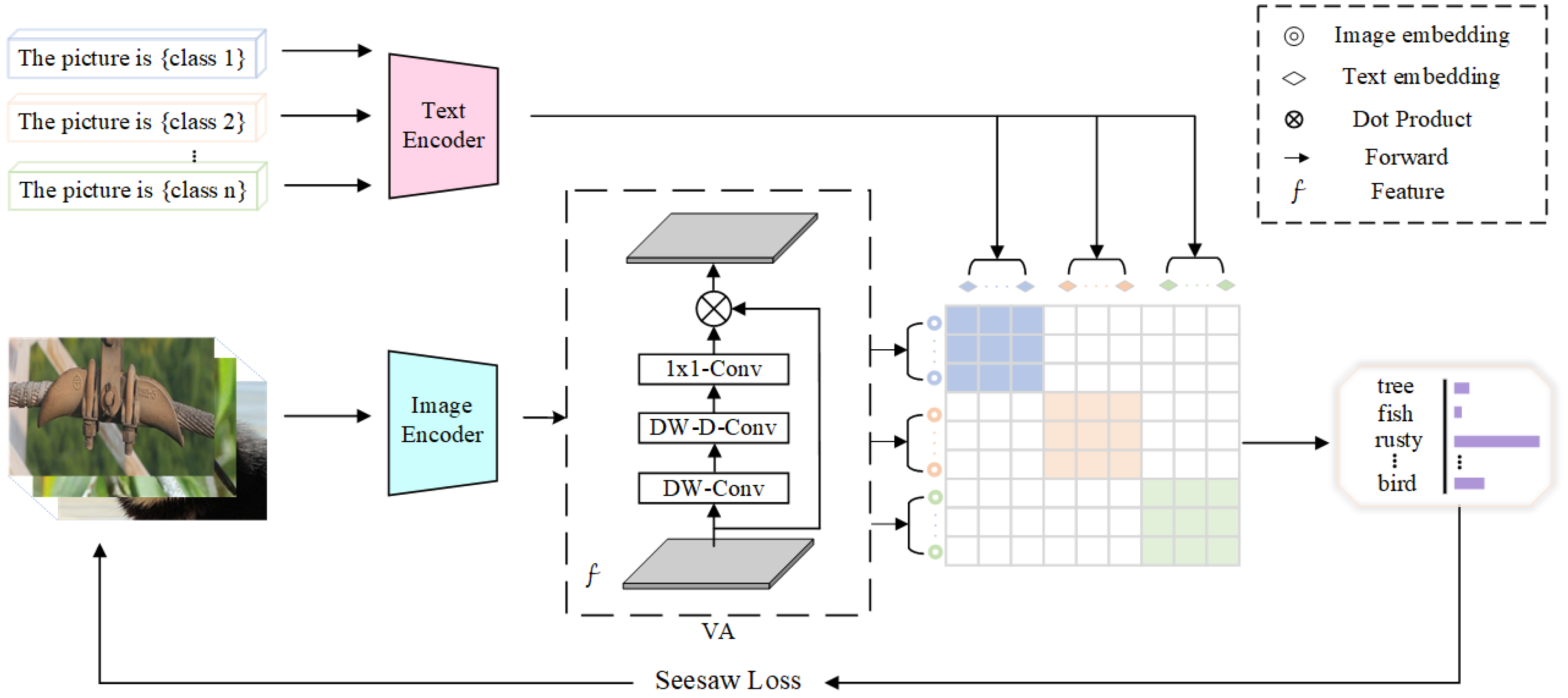
Recently, excellent work has been carried out alongside the rise in contrastive visual language learning, especially CLIP [45]. Multimodule visual models frequently learn the low-level properties of targets (e.g., their color, structure, and texture). In contrast, text models frequently display high-level semantic information and concepts, enabling them to serve as highly effective supplemental solutions for unbalanced data. However, this type of model is less effective in real-world scenarios due to the gap between visual and text representations and the lack of robustness to noisy text. CLIP compares 400 million image–text pairs collected from the web to produce consistent visual text representations, revitalizing the vision community. These robust visual-language representations derived from pretraining boost zero-shot classification performance in open-vocabulary settings without further annotations. We propose a simple visual language template for LTR, termed the text-to-image network (TIN), which is an end-to-end model that can combine the benefits of text and visual modules in visual tasks.

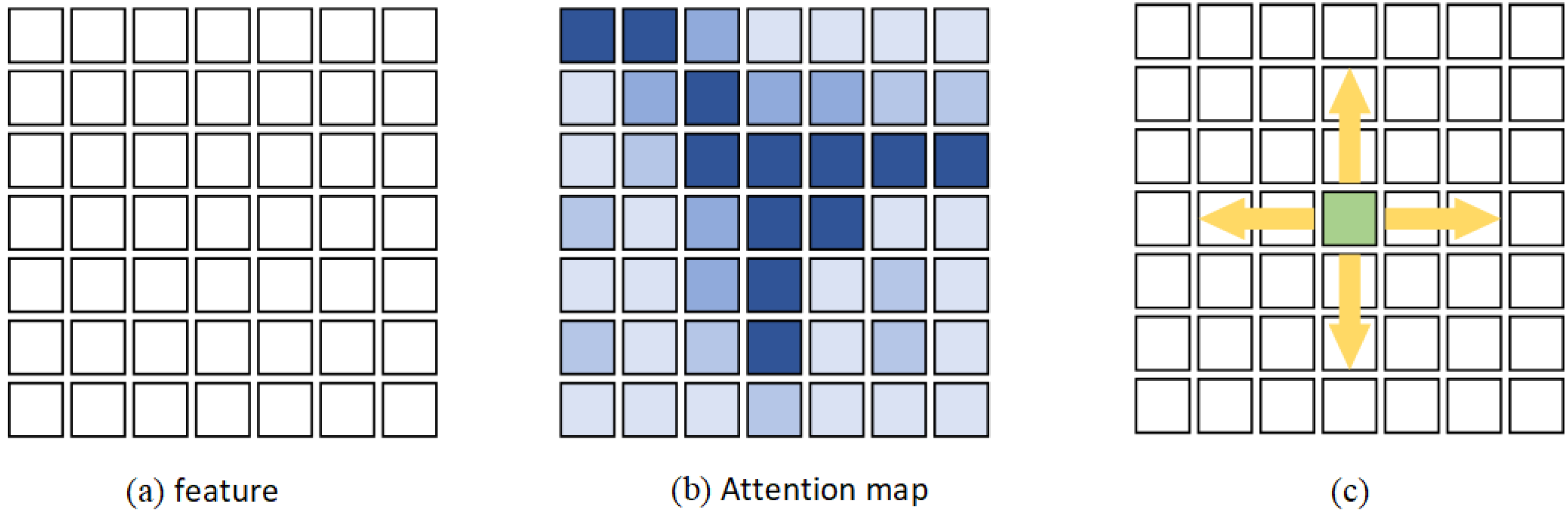
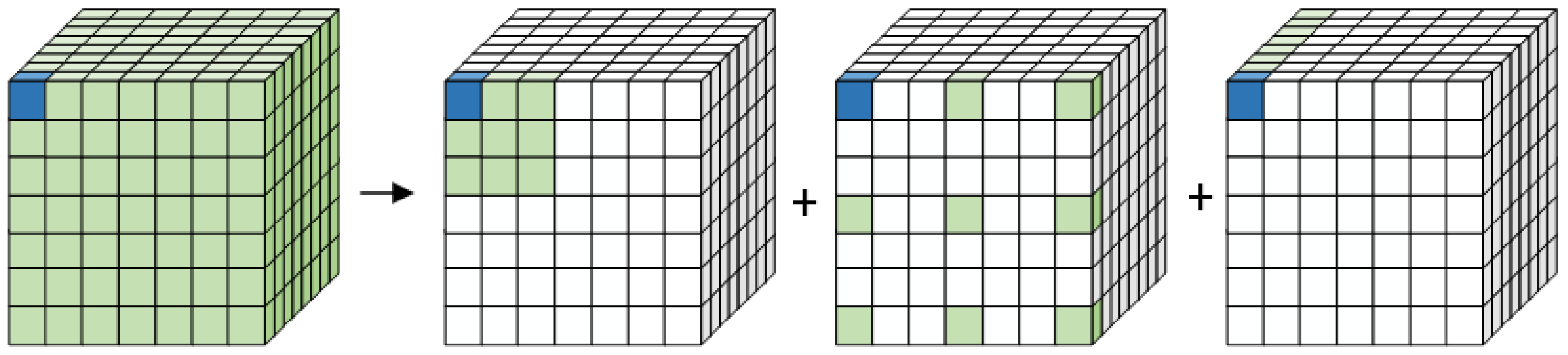
Our model has only one stage, saving a significant amount of processing time relative to two-stage models, and works well with imbalanced data. The primary process is as follows. We pretrained the model on the original unbalanced dataset and obtained language and visual expressions through comparative learning. Then, the large convolution kernel was split into three parts to generate an attention map and weigh the original image; this approach can better recognize the importance levels of different channels and ignore irrelevant parts [46]. 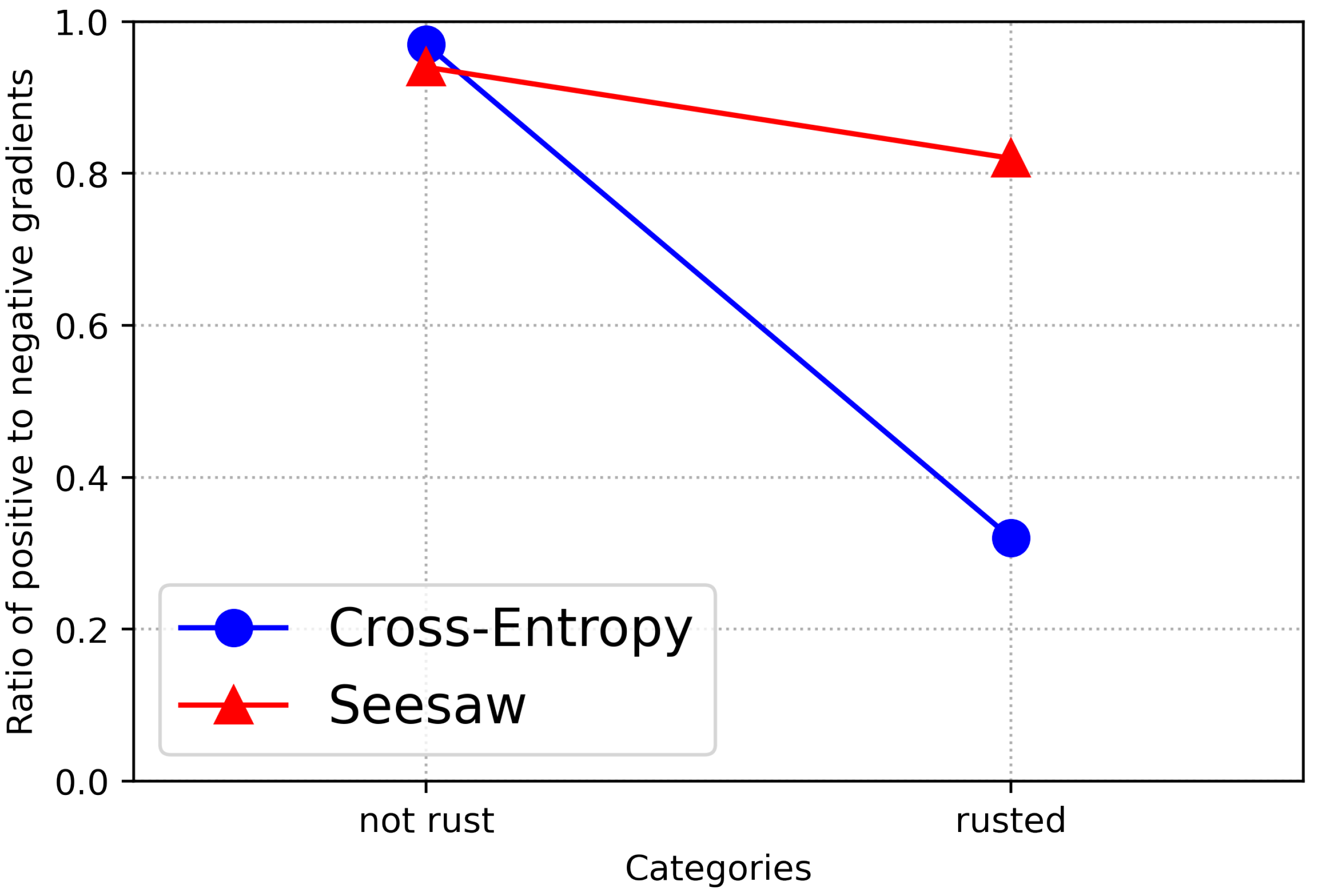This operation can save computational resources and estimate each channel’s importance when obtaining long-distance dependence, which is equivalent to combining the advantages of self-attention and squeeze-and-excitation (SE) attention [47]. A seesaw loss replaced the cross-entropy loss to better balance the two modules and long-tailed data [32]. Finally, classification results were obtained by matching the output text expression and image features using cosine similarity.

We performed extensive experiments on the clamp and ImageNet-LT datasets, and, in a fair comparison, our model outperformed the one-stage model by a considerable margin. In summary, our contributions are three-fold:

(1)

We pioneer the introduction of text-supervised signals from natural language processing in a computer-vision long-tailed dataset, and propose an end-to-end single-stage model, TIN, after combining visual supervision and textual information.

(2)

This innovative and simple template, TIN, consists of three main parts: two encoders, one for extracting text templates and the other for extracting picture features, and one visual attention method that can flexibly connect spatial location information and channel dimension importance. Ultimately, the seesaw loss function can suppress the negative gradient of the rare class and significantly improve the tail category, while only slightly sacrificing the accuracy of the head class. Unlike the previous individual visual information, we can combine visual features and text-supervised signals to conclude that the language and visual modules are complementary, especially in the case of sparse categories, effectively complementing the available information.

(3)

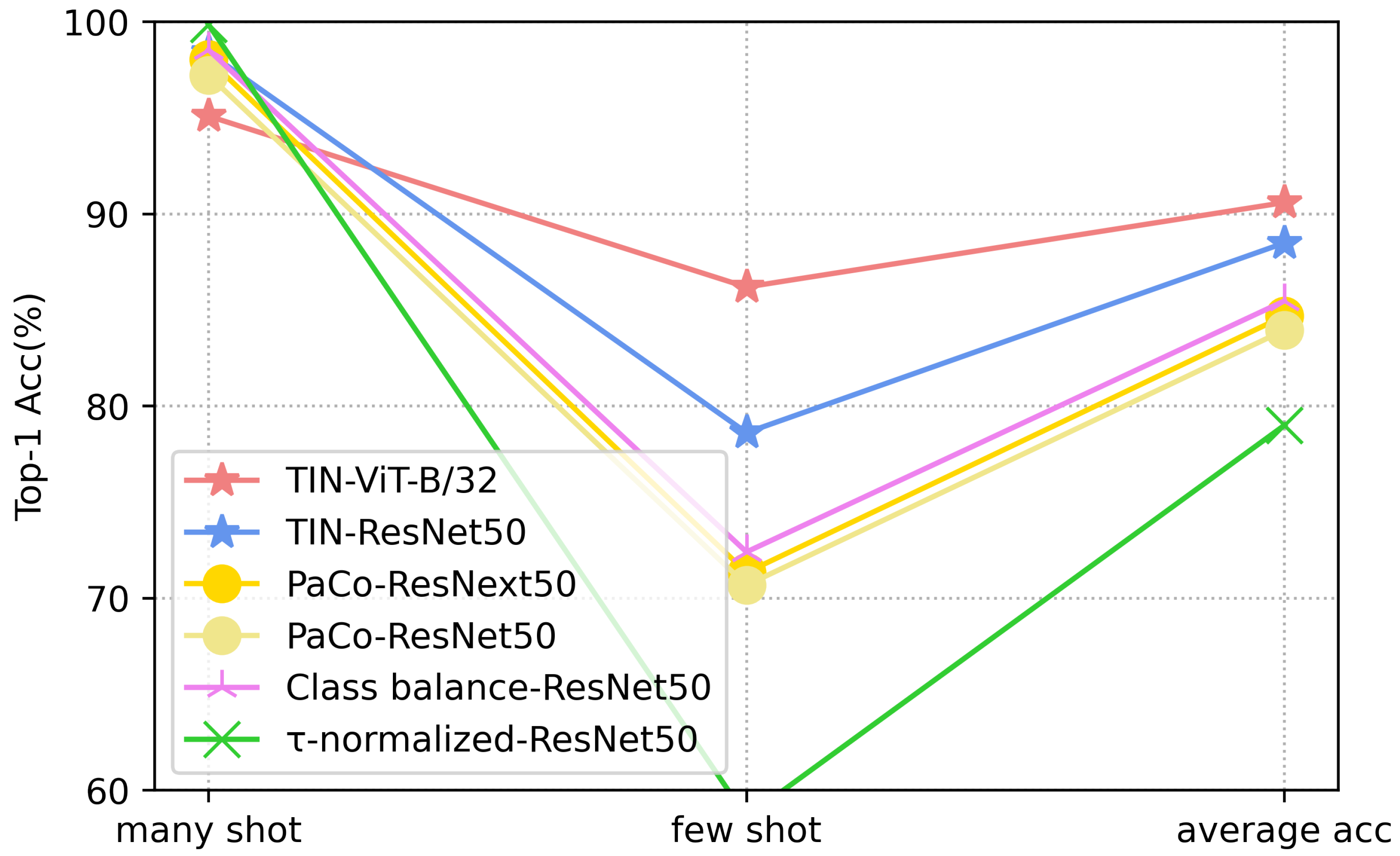
Using the clamp dataset, we conducted a comprehensive evaluation to demonstrate the effectiveness of the TIN, which substantially outperformed prior methods. Notably, we also conducted generalization experiments on the largest long-tailed dataset, ImageNet-LT, and TIN outperformed all single-stage advanced classifiers in recent years and achieved a state-of-the-art performance without bells and whistles.

2. Related Works

2.1. LTR

The distribution of training data in classic classification and identification tasks is typically artificially balanced, with no substantial variance in the sample numbers in different categories. A balanced dataset simplifies the algorithm’s robustness requirements, and somewhat ensures the reliability of the obtained model. However, as the number of categories expands, the cost of maintaining a balance exponentially increases.

We can obtain all the data naturally if we ignore the artificial equilibrium, i.e., the long-tailed dataset. Directly training for classification and detection tasks on these datasets will result in head data overfitting and tail data underfitting.

Resampling and reweighting are the two most basic long-tailed distribution solutions [19,25,26,27,28,29]. These strategies destroy the existing data distribution to fit an equilibrium function, i.e., by reverse weighting, strengthening the tail category learning process, and offsetting the long-tailed impact, thus reducing the effect of the head class to some extent. Moreover, some researchers have discovered that the image feature and category distributions are irrelevant. When learning to perform backbone feature extraction, we should avoid resampling with the category distribution and instead use the original data distribution [44]. Better outcomes can be achieved when extracting features in the first stage and retraining the employed classifiers in the second stage. Additionally, some academics believe that the head and tail classes have certain commonalities in transfer learning [48]. The visual information knowledge contained in head labels can be transferred to tail labels via a set of dynamic meta embeddings [49]. Some works have also created virtual samples to surround the tail samples to build a feature region, instead of the original feature points, e.g., a feature cloud, to relieve the problem of sample scarcity. For further information, see

Table 1. Summary of different learning approaches under class imbalances.

Method	Reference
Re-sampling	[19,25,26]
Re-weighting	[27,28,29]
Loss adjustment	[15,16,32]
Data augmentation	[35,42]
Decoupled training	[43,44]
Transfer learning	[33,34,48,49]

for details.

2.2. Vision-Language Models

Visionl-Language models are mainly divided into single-stream models and two-stream models. A single-stream model combines picture and text embeddings and feeds the result into a transformer model. On the other hand, a two-stream model allows the visual and text sides of the input data to be encoded separately using two independent transformers, where attention is inserted in the intermediate layer between the two encoders to merge the multimodule information.

The visual encoder method primarily extracts features from images and feeds them into a multimodule model. This primarily consists of three aspects: object detection (OD)-based region features, convolutional neural network (CNN)-based grid features, and vision transformer (ViT)-based patch features. OD-based region features identify the target region in the given image using a pretarget detection model and extract the representation of each region as the image side input. CNN-based grid features use CNN models such as ResNet to extract information from the original image [11], tile the final CNN input features into a sequence, and feed them into the multimodule model. ViT-based patch features extract picture information using the patch embedding approach as a reference [50].

VisualBERT splices text and image embedding sequences and feeds them into a transformer network using a single-stream model structure [51]. The network needs to clarify whether each embedding comes from a text measurement, an image measurement, or a position embedding. Then, the OD-based region feature extraction strategy is used to identify the target area on the image side and identify the results as the inputs for the next step. The text token is masked in one stage, and then the masked text is forecasted using additional text and image information in the next stage. Finally, the approach evaluates whether the image and text are consistent. Unicode-VL describes location data more thoroughly, creating a five-dimensional vector for each region [52]. The first four dimensions show the region’s position with respect to the complete image, and the fifth dimension represents the region’s size in proportion to that of the original image. VL-BERT adds a visual feature embedding module to the input, using the original image to improve the text encoding [53]. ImageBERT collects images and text from a website and ranks the positive sample pairings to incorporate more weakly supervised data and boost the learning effect [54]. Uniter calculates the corresponding relationship between the image and text embeddings via optimal transport [55]. In mask tasks, a sample only masks one module at a time during mask operations to avoid blocking critical information.

Lxmert [56], an OD-based two-stream model, employs two encoders to encode pictures and words and an interactive transformer to fuse the two data streams. Instead of using the OD technique, Pixel-BERT employs a CNN to extract the characteristics of the original picture and then splices the image and text embeddings into the model, drastically reducing the model’s complexity [57]. CLIP uses comparison learning to calculate the similarities between pictures and labels by gathering 400 million image–text pairs from the Internet as pretraining data; this approach has spawned a slew of CLIP-based models [45].

In this research, we demonstrate the effectiveness of CLIP in long-tailed data and the benefits of comparative learning compared to standard classifiers. As a result, we offer a CLIP-based single-stage network, which improves the essential information between channels using visual attention, adjusts the weight balance via the seesaw loss, and achieves a more balanced performance across all categories.

3. Methodology of TIN

This section provides a high-level summary of how the proposed multimodule model TIN addresses the long-tailed problem.

3.1. Overall Architecture

Our proposed model was implemented in an end-to-end manner without requiring secondary training and retuning, as illustrated in Figure 1. First, a pretraining CLIP model extracts picture and text features and then merges them into a single-latitude space. Previous attempts based on multiself-attention (MSA) were fruitful [58], but they overlooked the role of channels while focusing on the link between long and short distances. In this paper, the larger convolution block was divided into three steps using visual attention to reduce the number of calculations and obtain the attention map of every point [46]. When the attention map and original characteristics are weighted, the visual feature map can highlight the target features while weakening irrelevant information. The seesaw loss can update the logit based on the label frequencies, ensuring that the results are consistent with the distribution of the dataset. Ultimately, we conducted a similarity match between the output of the CNN network and the output of the transformer to obtain the final classification result.

3.2. Contrastive Learning Model

The success of the GPT series [59] in natural language processing (NLP) proves that learning from web-scale data can yield better results than good manual annotation [60]; however, this strategy is ignored in the computer vision (CV) field. CLIP establishes a link between image and text via a visual encoder and a text encoder, and then trains the model on 400 million pairs of image and text-in-text pairs of network data, with the aim of learning the representation of images from text. This very large training dataset offers CLIP the powerful ability to learn features and provides it with a zero-shot nature, making it unparalleled in its adaptability to the environment and allowing for good results to be obtained by direct inference on different datasets. The two encoders process text and image data separately, with the text encoder using Transformer and the image encoder using two models, ResNet or Vision Transformer (ViT). The visual encoder accepts an image as input and the text encoder accepts a text sentence as input, e.g., ’The image is a {label}’. The subsequent process can be divided into several steps. First, the image encoder and text encoder are used to map an image $I={\left\{I_i\right\}}_{i=1}^N$ and all label templates $T={\left\{T_i\right\}}_{i=1}^N$ to different spatial dimensions, where N denotes the batch size, i.e., $f_v=E_i^I\left(I_i\right)\in {\mathbb{R}}^{d_v}$, $f_t=E_i^T\left(T_i\right)\in {\mathbb{R}}^{d_t}$. The features of the two modules are mapped to the same embedding space and normalized through the dimension matrices $D_v\in {\mathbb{R}}^{d_v\times d}$ and $D_t\in {\mathbb{R}}^{d_t\times d}$:

$$V={\displaystyle \frac{D_v^T{f}_v}{\left|\right|D_v^T{f}_v\left|\right|}},T={\displaystyle \frac{D_t^T{f}_t}{\left|\right|D_t^T{f}_t\left|\right|}}$$

(1)

where V and T represent the normalized visual and textual features of the same dimension, respectively, and N represents the number of image–text pairs in the batch. Then, we optimize the two encodes via a contrastive learning loss, which can be formulated as:

$$\begin{array}{cc}\hfill {\mathcal{L}}_{v-t}=& {\mathcal{L}}_{vis}+{\mathcal{L}}_{text}\hfill \\ \hfill =& -{\displaystyle \frac{1}{N}}\sum _i^{N}log{\displaystyle \frac{exp\left(V_i^T{T}_i/\tau \right)}{{\sum }_{j=1}^{N}exp\left(V_i^T{T}_j/\tau \right)}}\hfill \\ \hfill & -{\displaystyle \frac{1}{N}}\sum _i^{N}log{\displaystyle \frac{exp\left(T_i^T{V}_i/\tau \right)}{{\sum }_{j=1}^{N}exp\left(T_i^T{V}_j/\tau \right)}}.\hfill \end{array}$$

(2)

The overall training goal was to maximize the high similarity score and decrease the mismatch score when coping with matching losses from two separate directions. ${\mathcal{L}}_{vis}$ and ${\mathcal{L}}_{text}$ denote the loss of the visual and language sides, respectively, and $\tau$ is the temperature parameter.

3.3. Visual Attention

Self-attention was first effectively used in NLP [58]. However, it has recently shown promise in CV, capturing both long- and short-distance dependencies and exhibiting the ability to spatially adjust. However, three faults remain when simply transferring self-attention from NLP to CV:

(1)

Limitation of dimensions: Self-attention is good at processing a one-dimensional sequence structure, but ignores the image’s two-dimensional structural information if it is directly employed for analysis.

(2)

Limitation of model complexity: Processing high-resolution images is difficult due to the complexity of self-attention.

(3)

Concerns about spatial and channel inconsistencies: The self-attention mechanism only considers spatial adaptation and ignores the channel dimension (e.g., the success of SENet).

Convolution, as opposed to the self-attention method, can fully extract an image’s 2D structural information, as shown in Figure 2; therefore, we can combine the advantages of both techniques to design the network.

As shown in Figure 3, the large convolution kernel is split into three operations that can reduce computational expense and generate long- and short-distance dependencies without self-attention [46]. One $K\times K$ large kernel convolution, for example, can be broken down into a ${\displaystyle \frac{K}{d}}\times {\displaystyle \frac{K}{d}}$ depthwise convolution, a $\left(2d-1\right)\times \left(2d-1\right)$ depthwise convolution, and a 1 × 1 pointwise convolution. According to the obtained attention map, the importance of each point can be judged, and the attention formula can be simplified as follows:

$$\begin{array}{cc}\hfill Attention=& Conv\left(input\right)\hfill \\ \hfill =& Con{v}_{1\times 1}\left(DW-D-Conv\left(DW-Conv\left(F\right)\right)\right),\hfill \end{array}$$

(3)

$$Output=Attention⨂F,$$

(4)

where $F\mathrm{and}Attention\in {\mathbb{R}}^{C\times H\times W}$, and then the dot product between Attention and F, are used to obtain the output.

3.4. Loss Function

The head class accounts for most of the samples in the long-tailed dataset, whereas the tail class accounts for only a minor portion. Therefore, the samples from the head category impose enormous negative gradients on the tail categories during training, swamping the positive gradients from the tail categories themselves. The classifier tends to deliver low responses to the tail categories to minimize the training loss incurred due to the uneven learning process.

For the single-label classification problem, we revisited the concept and formulation of the cross-entropy loss function. Each sample can only have one label in some tasks, such as the ImageNet image classification task or the MNIST handwriting digit recognition dataset [18]. For a single sample, the loss function is calculated as follows:

$$\begin{array}{c}\hfill L_{ce}=-\sum _{i=1}^n{y}_{i}log\widehat{y_i},\widehat{y_i}={\displaystyle \frac{e^{z_i}}{{\sum }_{j=1}^n{e}^{z_j}}},\end{array}$$

(5)

where n is the label, $y_i$ is the one-hot encoding, $z=[z_1,z_2,\cdots ,z_n]$ is the logit of each category, and $\widehat{y_i}$ is the predicted probability.

$${\displaystyle \frac{\partial L_{ce}\left(\mathbf{z}\right)}{\partial z_i}}=\widehat{y_i}-1$$

(6)

$${\displaystyle \frac{\partial L_{ce}\left(\mathbf{z}\right)}{\partial z_j}}=\widehat{y_j}$$

(7)

When i is the head label, and j is the tail label, the classifier applies a higher penalty to class j under the action of the loss function, and the prediction probability becomes massively skewed toward the head class.

By decreasing the weights of uncommon negative samples, the seesaw loss equalizes the gradient [32]. In this paper, we simplify the seesaw loss, and the formula is as follows:

$$\begin{array}{c}\hfill L_{seesaw}\left(\mathbf{z}\right)=-\sum _{i=1}^n{y}_{i}log\widehat{y_i},\\ \hfill \widehat{y_i}={\displaystyle \frac{e^{z_i}}{{\sum }_{j\ne 1}^n{M}_{ij}{e}^{z_j}+e^{z_i}+eps}},\end{array}$$

(8)

$$\begin{array}{c}\hfill \frac{\partial L_{seesaw}\left(\mathbf{z}\right)}{\partial z_j}=M_{ij}{\displaystyle \frac{e^{z_j}}{e^{z_i}}}\widehat{y_i}\end{array}$$

(9)

where $m_{ij}$ is the adjustment factor; $eps=1\times {10}^{-6}$ is used to prevent NaN values. The negative sample gradient of sample i to sample j can be expressed as Equation (9).

Mitigation Factor: According to the collected samples, the seesaw loss can continually adjust the samples in each category. This work supplies the corresponding amount of data as prior knowledge to speed up model training. As shown in Equation (9), the adjustment factor decreases the penalty for negative samples in a type when the number of samples of type i is greater than the number of samples of type j; otherwise, the adjustment factor is set as 1. The exponent p is a hyper-parameter that adapts the magnitude of mitigation.

$$M_{ij}=\left\{\begin{array}{c}1,if{N}_i⩽N_j\hfill \\ {\left({\displaystyle \frac{N_j}{N_i}}\right)}^p,if{N}_i>N_j\hfill \end{array}\right.$$

(10)

During the ResNet training process on the clamp dataset [11], we can determine the distribution of the cumulative gradients of positive and negative samples imposed on each class of classifiers, as shown in Figure 4. The positive-to-negative sample gradient ratio is close to 1.0 for the rust category and is very small for the rare rust label. As the quantity of samples decreases, the classification accuracy dramatically decreases, impacting the model performance. However, the seesaw loss can obtain better outcomes by more effectively balancing the positive and negative gradient ratios.

4. Experiments

4.1. Datasets

Engineers formed the clamp dataset according to the requirements of the National Grid. This dataset contains only two categories: rusty and not rusted. We only used a portion of the data for the experiment to speed up the training process, and the related data information is presented in

Table 2. Distribution of the original clamp dataset.

Train Set		Test Set
not rusted	rusty	not rusted	rusty
11,614	283	2566	58

.

The gap between the two categories is almost 50 times the number of rusty samples, which is a challenge for traditional classification models. Compared with the thousands of categories in an open dataset, a dataset with only two categories lowers the fault tolerance rate. We also conducted trials on ImageNet-LT, the largest long-tailed public dataset, to evaluate the model’s generalization ability. ImageNet-LT is a subset of the ImageNet dataset that contains 115.8K images from 1000 categories, with a maximum of 1280 images per class and a minimum of 5 [14].

4.2. Implementation Details

Due to the proposal of CLIP [45], we used CLIP as the backbone of the model. We tested the visual feature extraction abilities of ResNet-50 and ViT-B/32. The results refer to ViT-B/32 unless otherwise specified. The optimizer was trained on two Nvidia 3090 graphics cards using the most commonly used stochastic gradient descent (SGD) method, with a momentum of 0.9 and a batch size of 128. A cosine function was used to decay the learning rate scheme. Only the most basic data augmentation methods, such as rotation, cropping, and color conversion, were used in this research, and the initial learning rate is $1\times {10}^{-4}$. The input image was uniformly cropped to $224\times 224$ before being passed into the model, and the outcome was directly exported through the associated module. We only trained the TIN for 50 epochs, with the seesaw loss mitigation factor set to 0.7. Random seeds were set in the experiment to ensure reproducibility.

4.3. Evaluation Metrics

Each class adopted the top-1 accuracy metric to evaluate the accuracies achieved for the different datasets. These classes were divided into three subsets, the many-shot, medium-shot, and few-shot sets, which were determined by the number of instances in each category—more than 100 photographs, 20–100 images, and fewer than 20 images, respectively. Because the clamp dataset only has two categories, the rusty label and the not rusted label were divided into many-shot, few-shot, and medium-shot sections (the latter were deleted).

4.4. Performance Comparison

This section compares the performance of the TIN on the clamp dataset and those of the existing standard LTR algorithms.

Clamp Dataset:

Table 3. Results obtained using the clamp dataset.

Method	Backbone	Epochs	Many	Few	Average
$\tau$-normalized [44]	R-50	100	99.87	58.61	79.01
	R-101	100	98.45	60.30	79.38
	R-152	100	98.76	61.65	80.205
	X-50	100	99.31	59.69	79.50
	X-101	100	98.62	62.57	80.59
	X-152	100	99.78	64.80	82.29
Focal loss [61]	R-50	100	99.96	36.21	68.09
	R-101	100	99.51	41.38	70.45
	R-152	100	98.81	58.62	78.72
	X-50	100	99.26	24.14	61.70
	X-101	100	98.89	53.45	76.17
	X-152	100	99.14	25.86	62.50
Class balance [62]	R-50	100	98.55	72.41	85.48
	R-101	100	99.30	55.17	77.24
	R-152	100	99.38	62.07	80.73
	X-50	100	98.97	63.79	81.38
	X-101	100	99.38	60.34	79.86
	X-152	100	98.69	62.07	80.38
PaCo [63]	R-50	100	97.23	70.68	83.96
	X-50	100	98.06	71.34	84.70
TIN (Ours)	R-50	50	98.41	78.62	88.51 (+3.81)
	ViT-B/32	50	96.15	86.21	91.18 (+10.8)

The accuracy outcomes of several backbones and methodologies are compared using the clamp dataset. "R-*" and "X-*" stand for the ResNet [11] and ResNext [64] backbones, respectively. Compared to these algorithms, our model has a more significant advantage.

illustrates the LTR results of each technique, where our minimal baseline outperformed the previously developed single-stage models. By gradually increasing the size of the visual backbone, we found that the performance of the TIN also enjoys an improvement. When ResNet-50 is used as the backbone, the accuracy improves by $+3.81\%$, and when the maximum ViT-B/32 is employed, the accuracy improves by $10.8\%$, enabling our approach to outperform other one-stage models by a large margin. We plotted Figure 5, which clearly shows the gap between the models. In addition, the loss function and accuracy variation of the training process are shown in Figure 6 and Figure 7.

ImageNet-LT Dataset: We further verified the generalization ability of the proposed model on ImageNet-LT. As shown in

Table 4. Results obtained on ImageNet-LT.

Method	Backbone	Epochs	Many	Medium	Few	All
$\tau$-normalized [44]	R-50	90	56.6	44.2	27.4	46.7
LWS [44]	R-50	90	57.1	45.2	29.3	47.7
NCM [44]	R-50	90	58.9	46.6	31.1	49.2
cRT [44]	R-50	90	63.3	47.2	27.8	50.8
RIDE [49]	R-50	100	66.2	52.3	36.5	55.4
PaCo [63]	R-50	400	65.0	55.7	38.2	57.0
	X-50	400	67.5	56.9	36.7	58.2
TIN (Ours)	ViT-B/32	50	77.2	71.3	65.4	72.8 (+14.6)

, we chose ViT-B/32 as the backbone of the visual model for comparative experiments. We observes that, with only 50 training epochs, the TIN outperforms existing single-stage methods by 14.6%. Moreover, a 27.2 point improvement was achieved in the few-shot case, and the overall accuracy reached 72.8%, which is a state-of-the-art result for a single-stage model.

Places-LT Dataset: We performed additional generalizability studies on Place-LT, another large, long-tailed dataset. As shown in the

Table 5. Results obtained on Places-LT.

Method	Backbone	Many	Medium	Few	All
$\tau$-normalized [44]	R-50	34.5	31.4	23.6	31.0
LWS [44]	R-50	36.0	32.1	20.7	31.3
NCM [44]	R-50	37,1	30.6	19.9	30.8
cRT [44]	R-50	38.5	29.7	17.6	30.5
PaCo [63]	R-152	36.1	47.9	35.3	41.2
TIN (Ours)	ViT-B/32	46.2	43.6	35.8	42.3 (+1.1)

, our model shows some improvements over other single-stage models, but the improvement was not very significant, probably because the long-tailed distribution is more severe in this dataset than in ImageNet-LT.

5. Ablation Studies

In this section, we conduct several ablation experiments on our model. Finally, we illustrate the effectiveness of our strategy by fine-tuning the pretrained model, loss function, and visual attention mechanism.

5.1. Influence of the Pretrained Weights

The impacts of the CLIP weights and random initialization on the model are shown in

Table 6. Ablations results obtained with pretrained vision-language weights on the clamp dataset.

Vision	Language	Many	Few	Average
random	random	52.8	0.0	26.4
random	CLIP	53.7	0.0	26.7
CLIP	random	80.6	21.3	51.0
CLIP	CLIP	96.1	86.2	91.2

. As demonstrated by four studies, CLIP initialization significantly influences the accuracy, particularly for the visual encoder. When random initialization is used, the visual encoder learns more target characteristics than it does when utilizing the text encoder. Furthermore, the low performance of random initialization is due to the short training period (50 epochs), which makes convergence difficult. The advantage of contrastive vision-language models is demonstrated in this experiment.

5.2. Fine-Tuning the CLIP Backbone

At the same time, we conducted related research by fine-tuning the parameters of contrastive vision-language models, as shown in

Table 7. Ablation results obtained when fine-tuning on CLIP.

Vision	Language	Many	Few	Average
×	×	67.4	35.6	51.5
✓	×	88.4	76.8	82.6
×	✓	88.6	72.0	80.3
✓	✓	96.1	86.2	91.2

. In the table, × represents the freezing of encoder weights, and √ represents the fine-tuning of parameters. When both encoders are frozen, the model performs zero-shot inference. The table shows that, for the few-shot category, the visual module can lead to greater improvements in accuracy than the text module alone. This observation is highly similar to the conclusion of the previous experiment, which also demonstrates that, in the CV field, the language module is more lof a supplement, and adding thid when the model accuracy is saturated can raise the upper limit to a certain extent.

5.3. Fine-Tuning the Hyperparameter

In

Table 8. Ablation results involving the hyper-parameter p in the loss function of the mitigation factor.

p	Many	Few	Average
0.2	98.8	67.2	83.0
0.3	98.0	77.5	87.8
0.4	97.0	82.4	89.8
0.5	95.3	77.5	86.4
0.6	95.1	86.2	90.7
0.7	96.1	86.2	91.2
0.8	95.1	84.5	89.8
0.9	93.7	85.7	89.7

, we investigate the impact of the mitigation factor hyper parameter on the loss function. The punishment for the rare category is controlled by p. When p is set too high, many false positives (FPs) appear. It is difficult to suppress the gradient imbalance caused by excessive negative samples if p is too small. As a result, the key to achieving a balance in accuracy is choosing a suitable parameter for the given dataset. When p is $0.7$, the few-category and average accuracies are maximized, while the many-class accuracy is slightly reduced.

5.4. Impact of Different Modules

Table 9. Ablation of the different module.

Module	Many	Few	Average
$+CLIP$	99.53	72.41	85.97
$+Seesaw$	96.34	82.75	89.55
$+VA$	96.05	86.21	91.18

probes the role of each module in the entire network. When the previously developed CLIP is introduced, the model is accurate enough to compete with popular algorithms. However, it is far from sufficient in long-tailed engineering projects. The key to the engineering challenge is correctly recognizing the rare class. The seesaw loss improves the few-category accuracy while only slighly sacrificing performance in the many-shot class, making it a very cost-effective trade-off solution. The pixels at different places in multiple channels are weighted using visual attention (VA), which boosts the visual module’s feature capability and leads to high engineering precision. Note that we simply selected a small section of the dataset, achieving giant leaps in performance as we continued to increase the data size.

Finally, we visualized the classification results, as shown in Figure 8. Our model was shown to be more accurate in the identification of rare classes than other algorithms. The recognition accuracies of other algorithms are seriously affected when the parts near the clamp are rusted, but the TIN always produces correct recognition results.

6. Conclusions

The work in this paper mainly proposes an end-to-end model called the TIN to solve the LTR problem in engineering. First, a text module was introduced as a supplementary part of the visual feature mechanism with CLIP, which provides the model with an inherent multimodule advantage. Then, visual attention further improved the feature extraction process by strengthening the correlations between pixels in different channels. Finally, a seesaw loss was used to balance the weights between different categories. TIN achieved a state-of-the-art performance without bells and whistles on both datasets, outperforming the advanced classifiers developed in recent years. This demonstrates that text-supervised signals are important in the field of vision, especially in LTR, and can be an effective means of complementing the existing information. This work focuses on long-tailed image classification tasks, but the proposed approach is generalizable and may benefit other applications. For example, TIN can be applied to an image segmentation task. We can design a set of keywords that correspond to different detection categories in the image segmentation task. Since the final output feature map of the segmentation task is the same size as the input and has a high level of fine-grained information, we can match the similarities between each layer of the segmented feature map with the keywords to achieve better classification results. Although the proposed TIN achieved a good performance on multiple long-tailed recognition benchmarks, it still has some flaws. First, due to the limited text corpus, our method heavily relies on the use of pre-trained weights to learn high-quality language representation. Second, these results are trained on two Nvidia 3090, which are demanding graphics cards that are not easy to deploy. To allow for a better use in industrial equipment, the latter could be used in an attempt to simplify the model in terms of model quantization and pruning.

References

1. Williams, D.F.; Roger, B.M. Accurate transmission line characterization. IEEE Microw. Guid. Wave Lett. 1993, 3, 247–249. [Google Scholar] [CrossRef]
2. Li, L. The UAV intelligent inspection of transmission lines. In Proceedings of the 2015 International Conference on Advances in Mechanical Engineering and Industrial Informatics, Zhengzhou, China, 11–12 April 2015; pp. 1542–1545. [Google Scholar]
3. McGill, P.B.; Ramey, G.E. Effect of suspension clamp geometry on transmission line fatigue. J. Energy Eng. 1986, 112, 168–184. [Google Scholar] [CrossRef]
4. Li, T.; Luo, B.; Liu, L.; Wu, T. Wind accident analysis of transmission line in China Southern Power Grid’s Coastal Regions. In Proceedings of the 2015 5th International Conference on Electric Utility Deregulation and Restructuring and Power Technologies (DRPT), Changsha, China, 26–29 November 2015; IEEE: New York, NY, USA, 2015. [Google Scholar]
5. Li, X.; Lian, Y. Design and implementation of UAV intelligent aerial photography system. In Proceedings of the 2012 4th International Conference on Intelligent Human-Machine Systems and Cybernetics, Nanchang, China, 26–27 August 2012; Volume 2. [Google Scholar]
6. Liu, W.; Anguelov, D.; Erhan, D.; Szegedy, C.; Reed, S.; Fu, C.Y.; Berg, A.C. Ssd: Single shot multibox detector. In European Conference on Computer Vision; Springer: Cham, Swizterland, 2016; pp. 21–37. [Google Scholar]
7. Redmon, J.; Divvala, S.; Girshick, R.; Farhadi, A. You only look once: Unified, real-time object detection. In Proceedings of the IEEE Conference on Computer Vision and Pattern Recognition, Honolulu, HI, USA, 21–26 July 2016; pp. 779–788. [Google Scholar]
8. Hu, K.; Weng, C.; Zhang, Y.; Jin, J.; Xia, Q. An Overview of Underwater Vision Enhancement: From Traditional Methods to Recent Deep Learning. J. Mar. Sci. Eng. 2022, 10, 241. [Google Scholar] [CrossRef]
9. Fan, M.; Lai, S.; Huang, J.; Wei, X.; Chai, Z.; Luo, J.; Wei, X. Rethinking BiSeNet for real-time semantic segmentation. In Proceedings of the IEEE/CVF Conference on Computer Vision and Pattern Recognition, Nashville, TN, USA, 20–25 June 2021; pp. 9716–9725. [Google Scholar]
10. Huynh, C.; Tran, A.T.; Luu, K.; Hoai, M. Progressive semantic segmentation. In Proceedings of the IEEE/CVF Conference on Computer Vision and Pattern Recognition, Nashville, TN, USA, 20–25 June 2021; pp. 16755–16764. [Google Scholar]
11. He, K.; Zhang, X.; Ren, S.; Sun, J. Deep residual learning for image recognition. In Proceedings of the IEEE Conference on Computer Vision and Pattern Recognition, Honolulu, HI, USA, 21–26 July 2016; pp. 770–778. [Google Scholar]
12. Sandler, M.; Howard, A.; Zhu, M.; Zhmoginov, A.; Chen, L.C. Mobilenetv2: Inverted residuals and linear bottlenecks. In Proceedings of the IEEE Conference on Computer Vision and Pattern Recognition, Salt Lake City, UT, USA, 18–23 June 2018; pp. 4510–4520. [Google Scholar]
13. Tan, M.; Le, Q. Efficientnet: Rethinking model scaling for convolutional neural networks. In Proceedings of the International Conference on Machine Learning, PMLR, Long Beach, CA, USA, 15–20 June 2019; pp. 6105–6114. [Google Scholar]
14. Liu, Z.; Miao, Z.; Zhan, X.; Wang, J.; Gong, B.; Yu, S.X. Large-scale long-tailed recognition in an open world. In Proceedings of the IEEE/CVF Conference on Computer Vision and Pattern Recognition, Long Beach, CA, USA, 15–20 June 2019; pp. 2537–2546. [Google Scholar]
15. Van Horn, G.; Perona, P. The devil is in the tails: Fine-grained classification in the wild. arXiv 2017, arXiv:1709.01450. [Google Scholar]
16. Buda, M.; Atsuto, M.; Maciej, A.M. A systematic study of the class imbalance problem in convolutional neural networks. Neural Networks 2018, 106, 249–259. [Google Scholar] [CrossRef] [PubMed] [Green Version]
17. Lin, T.Y.; Maire, M.; Belongie, S.; Hays, J.; Perona, P.; Ramanan, D.; Zitnick, C.L. Microsoft coco: Common objects in context. In European Conference on Computer Vision; Springer: Cham, Switzerland, 2014; pp. 740–755. [Google Scholar]
18. Krizhevsky, A.; Sutskever, I.; Hinton, G.E. Imagenet classification with deep convolutional neural networks. Commun. ACM 2017, 60, 84–90. [Google Scholar] [CrossRef] [Green Version]
19. Jiang, Z.; Chen, T.; Chen, T.; Wang, Z. Improving Contrastive Learning on Imbalanced Seed Data via Open-World Sampling. arXiv 2021, arXiv:2111.01004. [Google Scholar]
20. Miao, S.; Xia, M.; Qian, M.; Zhang, Y.; Liu, J.; Lin, H. Cloud/shadow segmentation based on multi-level feature enhanced network for remote sensing imagery. Int. J. Remote. Sens. 2022, 43, 5940–5960. [Google Scholar] [CrossRef]
21. Wang, Z.; Xia, M.; Lu, M.; Pan, L.; Liu, J. Parameter Identification in Power Transmission Systems Based on Graph Convolution Network. IEEE Trans. Power Deliv. 2022, 37, 3155–3163. [Google Scholar] [CrossRef]
22. Chen, B.; Xia, M.; Qian, M.; Huang, J. MANet: A multi-level aggregation network for semantic segmentation of high-resolution. Remote. Sens. Images 2022, 43, 5874–5894. [Google Scholar] [CrossRef]
23. Gao, J.; Weng, L.; Xia, M.; Lin, H. MLNet: Multichannel feature fusion lozenge network for land segmentation. J. Appl. Remote. Sens. 2022, 16, 1–19. [Google Scholar] [CrossRef]
24. Song, L.; Xia, M.; Weng, L.; Lin, H.; Qian, M.; Chen, B. Axial Cross Attention Meets CNN: Bibranch Fusion Network for Change Detection. IEEE J. Sel. Top. Appl. Earth Obs. Remote. Sens. 2023, 16, 32–43. [Google Scholar] [CrossRef]
25. Hu, H.; Wei, F.; Hu, H.; Ye, Q.; Cui, J.; Wang, L. Semi-supervised semantic segmentation via adaptive equalization learning. Adv. Neural Inf. Process. Syst. 2021, 34, 22106–22118. [Google Scholar]
26. Chang, N.; Yu, Z.; Wang, Y.X.; Anandkumar, A.; Fidler, S.; Alvarez, J.M. Image-level or object-level? A tale of two resampling strategies for long-tailed detection. In Proceedings of the International Conference on Machine Learning, PMLR, Online, 18–24 July 2021; pp. 1463–1472. [Google Scholar]
27. Peng, H.; Mingming, S.; Ping, L. Optimal Transport for Long-Tailed Recognition with Learnable Cost Matrix. In Proceedings of the International Conference on Learning Representations, Online, 3–12 November 2021. [Google Scholar]
28. Kini, G.R.; Paraskevas, O.; Oymak, S.; Thrampoulidis, C. Label-imbalanced and group-sensitive classification under overparameterization. Adv. Neural Inf. Process. Syst. 2021, 34, 18970–18983. [Google Scholar]
29. Hong, Y.; Han, S.; Choi, K.; Seo, S.; Kim, B.; Chang, B. Disentangling label distribution for long-tailed visual recognition. In Proceedings of the IEEE/CVF Conference on Computer Vision and Pattern Recognition, Nashville, TN, USA, 20–25 June 2021; pp. 6626–6636. [Google Scholar]
30. Park, S.; Lim, J.; Jeon, Y.; Choi, J.Y. Influence-balanced loss for imbalanced visual classification. In Proceedings of the IEEE/CVF International Conference on Computer Vision, Montreal, BC, Canada, 11–17 October 2021; pp. 735–744. [Google Scholar]
31. Tan, J.; Lu, X.; Zhang, G.; Yin, C.; Li, Q. Equalization loss v2: A new gradient balance approach for long-tailed object detection. In Proceedings of the IEEE/CVF Conference on Computer Vision and Pattern Recognition, Nashville, TN, USA, 20–25 June 2021; pp. 1685–1694. [Google Scholar]
32. Wang, J.; Zhang, W.; Zang, Y.; Cao, Y.; Pang, J.; Gong, T.; Lin, D. Seesaw loss for long-tailed instance segmentation. In Proceedings of the IEEE/CVF Conference on Computer Vision and Pattern Recognition, Nashville, TN, USA, 20–25 June 2021; pp. 9695–9704. [Google Scholar]
33. Park, S.; Hong, Y.; Heo, B.; Yun, S.; Choi, J.Y. The Majority Can Help The Minority: Context-rich Minority Oversampling for Long-tailed Classification. In Proceedings of the IEEE/CVF Conference on Computer Vision and Pattern Recognition, New Orleans, LA, USA, 18–24 June 2022; pp. 6887–6896. [Google Scholar]
34. Parisot, S.; Esperança, P.M.; McDonagh, S.; Madarasz, T.J.; Yang, Y.; Li, Z. Long-tail Recognition via Compositional Knowledge Transfer. In Proceedings of the IEEE/CVF Conference on Computer Vision and Pattern Recognition, New Orleans, LA, USA, 18–24 June 2022; pp. 6939–6948. [Google Scholar]
35. Zhou, A.; Tajwar, F.; Robey, A.; Knowles, T.; Pappas, G.J.; Hassani, H.; Finn, C. Do Deep Networks Transfer Invariances Across Classes? arXiv 2022, arXiv:2203.09739. [Google Scholar]
36. Yan, F.; Zhang, Z.; Liu, Y.; Liu, J. Design of Convolutional Neural Network Processor Based on FPGA Resource Multiplexing Architecture. Sensors 2022, 22, 5967. [Google Scholar] [CrossRef]
37. Yan, F.; Zhang, H.; Zhou, T.; Fan, Z.; Liu, J. Research on Multiscene Vehicle Dataset Based on Improved FCOS Detection Algorithms. Complexity 2021, 2021, 1–10. [Google Scholar] [CrossRef]
38. Hu, K.; Li, Y.; Xia, M.; Wu, J.; Lu, M.; Zhang, S.; Weng, L. Federated learning: A distributed shared machine learning method. Complexity 2021, 2021, 1–20. [Google Scholar] [CrossRef]
39. Hu, K.; Wu, J.; Li, Y.; Lu, M.; Weng, L.; Xia, M. Fedgcn: Federated learning-based graph convolutional networks for non-euclidean spatial data. Mathematics 2022, 10, 1000. [Google Scholar] [CrossRef]
40. Lu, C.; Xia, M.; Lin, H. Multi-scale strip pooling feature aggregation network for cloud and cloud shadow segmentation. Neural Comput. Appl. 2022, 34, 6149–6162. [Google Scholar] [CrossRef]
41. Qu, Y.; Xia, M.; Zhang, Y. Strip pooling channel spatial attention network for the segmentation of cloud and cloud shadow. Comput. Geosci. 2021, 157, 104940. [Google Scholar] [CrossRef]
42. Zhong, Z.; Cui, J.; Liu, S.; Jia, J. Improving calibration for long-tailed recognition. In Proceedings of the IEEE/CVF Conference on Computer Vision and Pattern Recognition, Online, 19–25 June 2021; pp. 16489–16498. [Google Scholar]
43. Alshammari, S.; Wang, Y.X.; Ramanan, D.; Kong, S. Long-tailed recognition via weight balancing. In Proceedings of the IEEE/CVF Conference on Computer Vision and Pattern Recognition, New Orleans, LA, USA, 18–24 June 2022; pp. 6897–6907. [Google Scholar]
44. Kang, B.; Xie, S.; Rohrbach, M.; Yan, Z.; Gordo, A.; Feng, J.; Kalantidis, Y. Decoupling representation and classifier for long-tailed recognition. arXiv 2019, arXiv:1910.09217. [Google Scholar]
45. Radford, A.; Kim, J.W.; Hallacy, C.; Ramesh, A.; Goh, G.; Agarwal, S.; Sutskever, I. Learning transferable visual models from natural language supervision. In Proceedings of the International Conference on Machine Learning, PMLR, Online, 18–24 July 2021; pp. 8748–8763. [Google Scholar]
46. Guo, M.H.; Lu, C.Z.; Liu, Z.N.; Cheng, M.M.; Hu, S.M. Visual attention network. arXiv 2022, arXiv:2202.09741. [Google Scholar]
47. Hu, J.; Shen, L.; Sun, G. Squeeze-and-excitation networks. In Proceedings of the IEEE Conference on Computer Vision and Pattern Recognition, Salt Lake City, UT, USA, 18–23 June 2018. [Google Scholar]
48. Zhu, L.; Yang, Y. Inflated episodic memory with region self-attention for long-tailed visual recognition. In Proceedings of the IEEE/CVF Conference on Computer Vision and Pattern Recognition, Seattle, WA, USA, 13–19 June 2020; pp. 4344–4353. [Google Scholar]
49. Wang, X.; Lian, L.; Miao, Z.; Liu, Z.; Yu, S.X. Long-tailed recognition by routing diverse distribution-aware experts. arXiv 2020, arXiv:2010.01809. [Google Scholar]
50. Dosovitskiy, A.; Beyer, L.; Kolesnikov, A.; Weissenborn, D.; Zhai, X.; Unterthiner, T.; Houlsby, N. An image is worth 16x16 words: Transformers for image recognition at scale. arXiv 2020, arXiv:2010.11929. [Google Scholar]
51. Li, L.H.; Yatskar, M.; Yin, D.; Hsieh, C.J.; Chang, K.W. Visualbert: A simple and performant baseline for vision and language. arXiv 2019, arXiv:1908.03557. [Google Scholar]
52. Li, G.; Duan, N.; Fang, Y.; Gong, M.; Jiang, D. Unicoder-vl: A universal encoder for vision and language by cross-modal pre-training. In Proceedings of the AAAI Conference on Artificial Intelligence, New York, NY, USA, 7–12 February 2020; Volume 34, pp. 11336–11344. [Google Scholar]
53. Su, W.; Zhu, X.; Cao, Y.; Li, B.; Lu, L.; Wei, F.; Dai, J. Vl-bert: Pre-training of generic visual-linguistic representations. arXiv 2019, arXiv:1908.08530. [Google Scholar]
54. Qi, D.; Su, L.; Song, J.; Cui, E.; Bharti, T.; Sacheti, A. Imagebert: Cross-modal pre-training with large-scale weak-supervised image-text data. arXiv 2020, arXiv:2001.07966. [Google Scholar]
55. Chen, Y.C.; Li, L.; Yu, L.; El Kholy, A.; Ahmed, F.; Gan, Z.; Liu, J. Uniter: Universal image-text representation learning. In European Conference on Computer Vision; Springer: Cham, Switzerland, 2020; pp. 104–120. [Google Scholar]
56. Tan, H.; Mohit, B. Lxmert: Learning cross-modality encoder representations from transformers. arXiv 2019, arXiv:1908.07490. [Google Scholar]
57. Huang, Z.; Zeng, Z.; Liu, B.; Fu, D.; Fu, J. Pixel-bert: Aligning image pixels with text by deep multi-modal transformers. arXiv 2020, arXiv:2004.00849. [Google Scholar]
58. Vaswani, A.; Shazeer, N.; Parmar, N.; Uszkoreit, J.; Jones, L.; Gomez, A.N.; Polosukhin, I. Attention is all you need. Adv. Neural Inf. Process. Syst. 2017, 30. [Google Scholar] [CrossRef]
59. Brown, T.; Mann, B.; Ryder, N.; Subbiah, M.; Kaplan, J.D.; Dhariwal, P.; Amodei, D. Language models are few-shot learners. In Advances in Neural Information Processing Systems 33; Neural Information Processing Systems Foundation, Inc.: La Jolla, CA, USA, 2020; pp. 1877–1901. [Google Scholar]
60. Brown, T.; Mann, B.; Ryder, N.; Subbiah, M.; Kaplan, J.D.; Dhariwal, P.; Neelakantan, A.; Shyam, P.; Sastry, G.; Askell, A.; et al. Language models are few-shot learners. Adv. Neural Inf. Process. Syst. 2020, 33, 1877–1901. [Google Scholar]
61. Lin, T.Y.; Goyal, P.; Girshick, R.; He, K.; Dollár, P. Focal loss for dense object detection. In Proceedings of the IEEE International Conference on Computer Vision, Venice, Italy, 22–29 October 2017; pp. 2980–2988. [Google Scholar]
62. Ren, J.; Yu, C.; Ma, X.; Zhao, H.; Yi, S. Balanced meta-softmax for long-tailed visual recognition. Adv. Neural Inf. Process. Syst. 2020, 33, 4175–4186. [Google Scholar]
63. Cui, J.; Zhong, Z.; Liu, S.; Yu, B.; Jia, J. Parametric contrastive learning. In Proceedings of the IEEE/CVF International Conference on Computer Vision, Montreal, BC, Canada, 11–17 October 2021; pp. 715–724. [Google Scholar]
64. Xie, S.; Girshick, R.; Dollár, P.; Tu, Z.; He, K. Aggregated residual transformations for deep neural networks. In Proceedings of the IEEE Conference on Computer Vision and Pattern Recognition, Honolulu, HI, USA, 21–26 July 2017; pp. 1492–1500. [Google Scholar]
Figure 1. Overview of our TIN template. We transmitted the original image and label templates to the vision-language backbone of the long-tailed data. Visual attention was used to assess long-distance dependencies, and the relevance of each channel was determined and reweighted to improve the visual features. The gradients were reweighted according to the label frequencies when the head class obtained several gradients. Finally, the accuracy of the tail class considerably improved while the accuracy of the head class slightly decreased.
Applsci 13 03287 g001
Figure 2. (a): The image input features; (b) the relevance of each point after visualization; (c) the value of the green point depends on the information about the known surrounding points.
Applsci 13 03287 g002
Figure 3. The standard large kernel convolution can be separated into three operations to decrease the number of computations, e.g., a depthwise convolution (DW-C), a depthwise division convolution (DW-D-C), and a pointwise convolution (PW-C). In the figure, blue is the center point, and green represents the range of convolution.
Applsci 13 03287 g003
Figure 4. Under the traditional cross-entropy loss, the head class’s positive and negative sample gradients are close to 1.0 while the sparse tail class is tiny, which will cause an accuracy bottleneck. The seesaw loss is adjusted by reducing the negative sample gradient of the tail class to obtain a more balanced gradient distribution.
Applsci 13 03287 g004
Figure 5. Comparison with the state-of-the-art approaches on Clamp dataset. TIN with ResNet-50 visual backbone outperforms models with a more complex structure and longer training epochs by a large margin.
Applsci 13 03287 g005
Figure 6. (a) Figure shows the accuracy of the unrusted (Many) category; (b) Figure shows the accuracy of the rusty (Few) category.
Applsci 13 03287 g006
Figure 7. The picture shows the loss reduction of the training process.
Applsci 13 03287 g007
Figure 8. Results visualization: The results of the other models and our network are shown in each picture’s upper left and right corners, respectively. Our model is more robust to rare classes and can recognize pictures more accurately.
Applsci 13 03287 g008