1. Introduction
With the arrival of the new energy era, there has been a sharp increase in demand for load use, and the characteristics of load fluctuations have also changed. To ensure the safety and efficiency of the power system, the role of load forecasting is becoming increasingly important. Short-term load forecasting is utilized to forecast the load value for the next day or several consecutive days. Its forecasting results can be used for economic load dispatching, equipment maintenance, water, heat and electricity coordination, and more. Improving load forecasting accuracy will help ensure a balance between power supply and demand, and improve the economy of economic dispatching and power generation equipment utilization. With the continuous advancement of smart grid data acquisition technology, the dimension of load characteristics is becoming larger, and the volatility and nonlinearity of load are becoming stronger. All of these factors increase the difficulty of load forecasting [
1].
Short-term power loads show strong randomness and volatility due to various factors such as climate, economic, and residential electricity consumption behavior. This increases the difficulty of load forecasting [
2]. Currently, short-term load forecasting methods can be classified into three categories: mathematical statistics-based forecasting models, traditional machine learning-based forecasting models, and deep learning-based forecasting models. Load forecasting based on mathematical–statistical models includes multiple linear regression, Kalman filter, exponential smoothing method, and more [
3]. Mathematical–statistical models have a clear statistical relationship between time, load, influencing factors, and past time load. The mathematical–statistical model is simple, and its prediction speed is fast. However, only simple and smooth time series can be suitable for this prediction method. For complex nonlinear load series, random factors can destroy the original prediction criteria of the model, leading to inaccurate prediction results [
4].
In traditional machine learning models, support vector regression (SVM), fuzzy systems, decision trees (DT), and linear regression (LR) are commonly used to predict power consumption [
5,
6,
7,
8]. Bogomolov et al. [
9] developed an improved random forest algorithm for weekly power prediction, while Yaslan et al. [
10] developed a hybrid model that combined mode decomposition and support vector regression for power consumption prediction. Aasim et al. [
11] proposed a hybrid model combining wavelet transform (WT) and support vector machine (SVM) for power load estimation. Barman et al. [
12] proposed a regional mixed STLF model that used SVM and the grasshopper optimization algorithm to estimate appropriate model parameters for load forecasting. Sulaiman et al. [
13] proposed a hybrid method based on empirical mode decomposition and extreme learning machine (ELM) to predict residential load based on smart meter data and compared it with traditional machine learning models to verify its effectiveness. Chen et al. [
14] proposed a short-term prediction algorithm based on the optimized ELM algorithm. Tang et al. [
7] built a forecasting algorithm based on the fuzzy system. Malekizadeh et al. [
15] used the fuzzy neural model to predict the hourly load distribution before the day. The model took into account the time distribution of temperature, and the parameters of the model do not need to be set in advance. Li et al. [
16] proposed a meta-learning algorithm for automatic distribution systems. The algorithm included three parts: extraction of features, preparation of model parameters, and online recommendation of models. Machine learning models perform well on simple datasets, but due to the collinearity of the independent variables of power consumption, these models have insufficient power consumption prediction ability. In addition, with the increase of data, these models usually have the problem of over-fitting.
With the vigorous research into deep learning for image recognition and speech recognition [
17,
18,
19,
20,
21], deep learning technology has been introduced into load forecasting. At present, there are mainly two kinds of prediction models based on CNN and the long LSTM model. Sadaei et al. [
22] proposed a load short-term prediction algorithm based on the fuzzy method and convolution neural network. It used the deep learning CNN model to extract relevant important parameters and fuzzy logic to represent the one-dimensional time series. Niu et al. [
23] qualitatively analyzed the multi-energy load relationship, screened the influencing factors of load prediction based on data-driven analysis, and proposed a new multi-energy load prediction algorithm based on the CNN-BiGRU algorithm. A prediction model using LSTM was proposed by Wang et al. [
24], in which autocorrelation graph was used for extracting hidden features. Hong et al. [
25] proposed a hybrid convolutional neural network (CNN) with cascaded networks to forecast the daily peak load, and tested it with data from Taiwan. This method was superior to the traditional model. Haque et al. [
26] proposed a regularized deep neural network method for short-term power load forecasting of commercial buildings and used it to forecast the power load of two commercial buildings in Virginia (30 min and 24 h ago). Moradzadeh et al. [
27] proposed a Bi-LSTM network for short-term load forecasting. In Moradzadeh’s work, the feature of time series was extracted by the multi-directional LSTM model, which improved the multi-dimensional expression ability of the time series features. Jiang [
28] proposed a new multi-behavior LSTM model with bottleneck characteristics. This model combined the prediction behavior and weekly features by applying the bottleneck technology to the energy management system. Chen et al. [
29] proposed a new deep residual network for load prediction. The network proposed a new deep residual network to address the issue of vanishing and exploding gradients in neural networks and to improve forecasting accuracy. Jiang et al. [
30] introduced a hybrid multi-task and multi-information fusion deep learning algorithm that takes into account short-term and long-term behavioral rules to achieve load forecasting. Similarly, the authors of [
31,
32] developed deep learning models, but they faced challenges in modeling the temporal and spatial characteristics of power data.
At present, the outstanding methods are mainly based on the deep learning model, which can automatically obtain the characteristics of the time series. However, the existing methods based on CNN are difficult to obtain the temporal correlation of the time series, and the existing models do not consider the multi-time scale characteristics of the load series. Although LSTM can extract temporal correlation, its feature extraction ability is weak. In addition, the importance of various factors affecting load power is different, and the existing methods do not distinguish these factors, which also affects the accuracy of prediction. In this paper, a multi-scale feature attention mixture network model (MFAMNet) was constructed to realize load forecasting, which makes full use of the time information and introduces the LSTM network into the model to extract the time correlation of the sequence. The multi-scale convolution neural network (CNN) is used to automatically extract the multi-scale features of the load, and a lot of information will not be lost in the dimensionality reduction. In addition, this paper constructs a two-branch attention mechanism to capture the important parameters of different influencing factors to improve the ability of the network for extracting effective features. The experimental results on two open test sets show that the proposed MFAMNet is superior to the existing SOTA load prediction methods.
2. Methods
This work proposes a mixture network combining CNN and LSTM, and adds attention mechanism and multi-scale mechanism to the hybrid model. The network can make full use of the ability of convolution neural networks to extract spatial features, long-term memory networks to extract time features, multi-scale convolution to achieve multi-scale feature extraction of time series, realizing the important expressions of different features through attention mechanisms.
CNN and LSTM are both important methods for time series analysis [
33]. The CNN algorithm can effectively extract the spatial features of data in a very abstract way [
34]. One-dimensional convolution of the convolution neural network can obtain the spatial structural characteristics of the sequence, i.e., the shape characteristics of the sequence, which can help improve the accuracy of prediction. The LSTM network can extend the temporal characteristics and process data with sequential characteristics. Therefore, combining the advantages of CNN and LSTM can form a new method that gives full play to their respective strengths. In this paper, the multi-scale feature attention mixture network model (MFAMNet) is obtained by combining the two networks to fully utilize temporal and spatial characteristics. The specific framework of the network is shown in
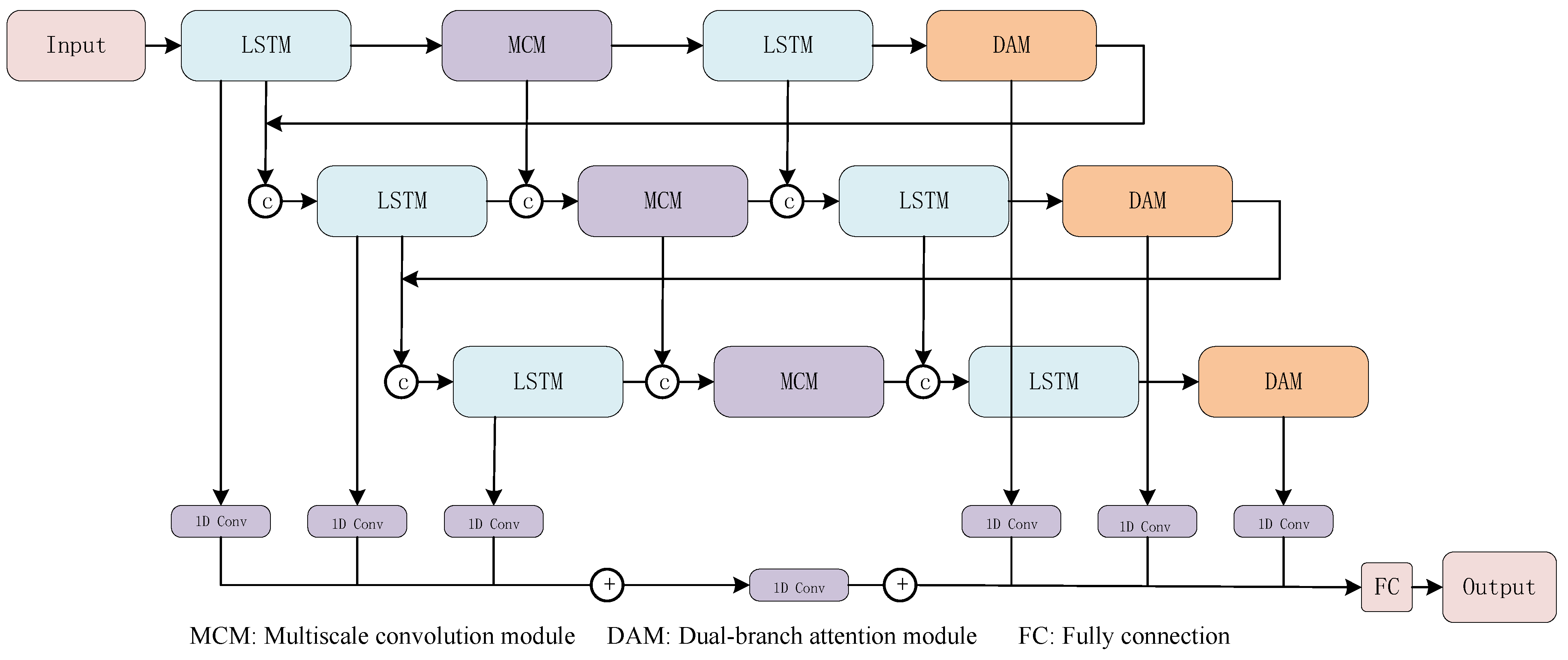
Figure 1.
As shown in
Figure 1, the data are first sent into the LSTM module, multi-scale convolution module, LSTM module, and residual attention module, and the operation is cycled three times. Then, the model selects the output of the first LSTM module and the residual attention module in each cycle and feeds them into a one-dimensional convolution. Finally, all the results are added to obtain the predicted results. The purpose of this structure is to enable the network to fully extract the features of multi-scale time series and make the network more capable of feature expression. This multi-level circular structure can extract the multi-level characteristics of the load, i.e., it effectively retains the temporal dependent features of the shallow-level load sequence and also obtains the deeper-level load characteristics. The network reshapes the multi-layer features through the attention mechanism and integrates them with the features at all levels, which greatly improves the diversity and effectiveness of network features, and can effectively express the phenomenon of load climbing and load shock. In particular, the extraction of data features of load peaks can be more sufficient, which is conducive to improving the ability of the network to conduct load forecasting. For household loads, the peak of the load often exists for a short time, so how to obtain the effective characteristics of the load peak will become particularly important, while in the traditional network, it is easy to ignore the features of the load peak because the proportion of the load peak in the whole sequence is too low.
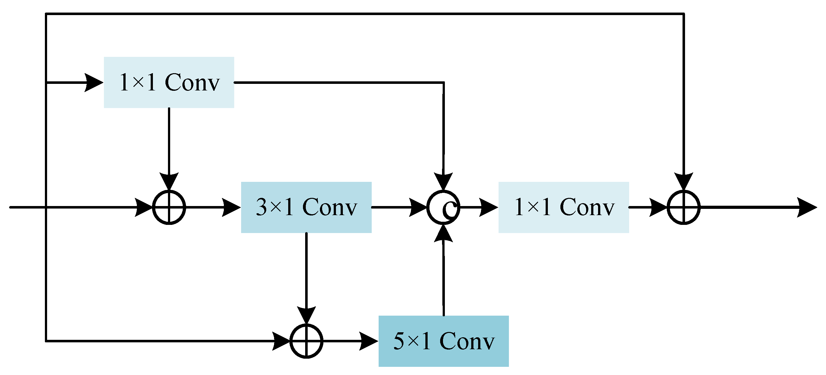
2.1. Multiscale Convolution Module
The convolution kernels in the traditional residual cell are the same sizes, which makes it impossible for the convolution layer to “observe” the load data from multiple scales, and it is difficult to obtain richer input features. To solve this problem, this paper adopts multi-scale convolution. The multi-scale structure of the backbone network is shown in
Figure 2.
The multi-scale convolution module has four branches in total. The first branch uses
convolution. The
convolution can increase the dimension and reduce the number of feature channels and uses a small amount of computation to increase the linear transformation and nonlinear transformation of features, so as to improve the expression ability of the network and improve the accuracy of load prediction. In the second branch, the original input and the input of the first branch are added and then convolved by
convolution, which is equivalent to two feature changes. In the third branch, the original input and the input of the second branch are added and then convolved by
, and then the outputs of the three branches are spliced on the channel dimension. After that, the concatenated result is dimensionally reduced through the
convolution module, so that it has the same number of channels as the original input. Finally, we add the output and the original input to obtain the final output. The specific calculation formula is as follows:
where
is the initial input data,
is the output feature,
a one-dimensional convolution with
,
a one-dimensional convolution with
,
a one-dimensional convolution with of
,
refers to the operation of stacking data on the channel dimension. The multi-scale convolution obtains multi-scale features of the load series and multi-scale features of other relevant information (including temperature, humidity, rainfall, etc.).
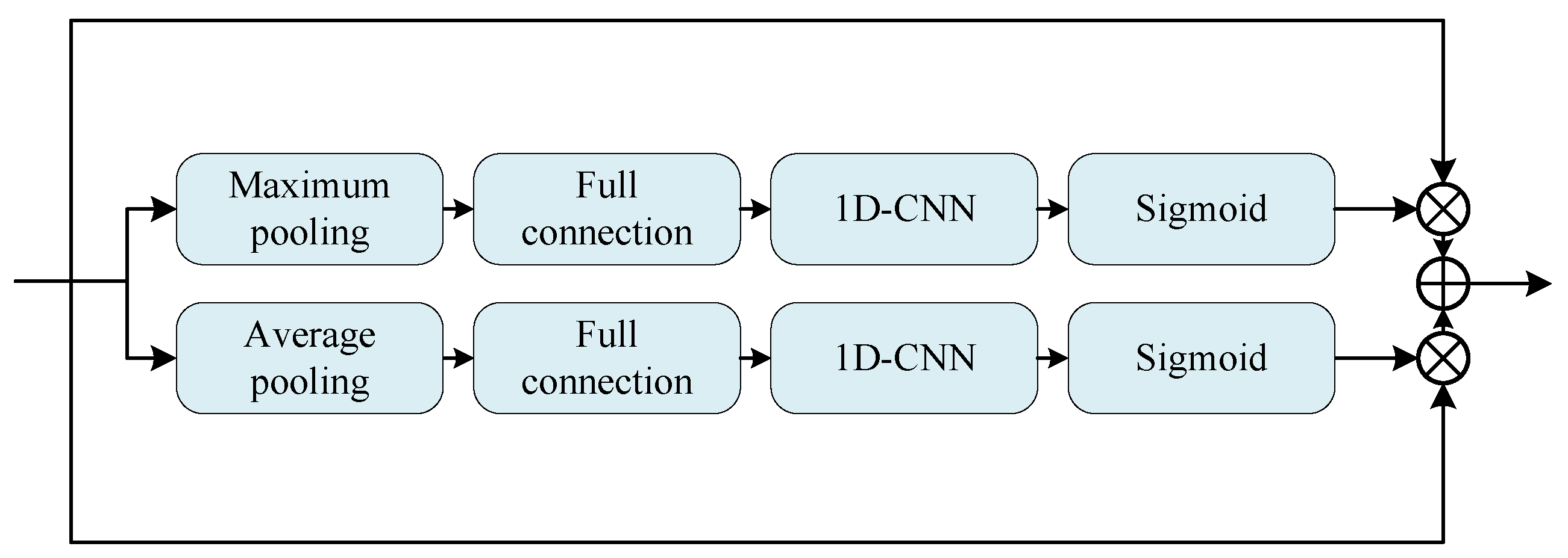
2.2. Dual-Branch Attention Module
In order to obtain a more powerful network and enable the network to give more important weight to important features, the dual-branch attention mechanism method is proposed in the residual unit, as shown in
Figure 3, which enhances the network’s learning ability of load characteristics from the channel level.
Firstly, the global average pooling and the global maximum pooling layer are used to compress the feature image from the spatial perspective, and the two-dimensional channel is transferred to a real number, which represents the global receptive field to some extent, representing the response to the global information of the feature channel. Then it is sent into the full connection layer, one-dimensional convolution, and sigmoid function, respectively. After that, we multiply the two results with the original data and add them together to obtain the final output. The specific calculation formula is as follows:
where
is the input feature,
is the output feature,
is global maximum pooling,
is global average pooling,
is full connection layer,
a one-dimensional convolution with
,
is the sigmoid function. The attention mechanism proposed will re-calibrate the rich features. The two-branch attention module can obtain the importance of each feature, and then enhance the useful information and suppress the information that is not important to the task according to the importance, which can also improve the ability of network load forecasting.
3. Results
This paper used AEP [
35] and IHEPC [
36] datasets to verify the proposed model. The AEP dataset includes 29 different characteristic parameters, such as temperature, wind speed, humidity, and electrical energy consumption. Data were collected from wireless sensors in indoor and outdoor environments. Outdoor data included temperature, humidity, pressure, and visibility. Indoor temperatures were collected from different locations, including the kitchen, living room, laundry, office, bathroom, etc. This dataset collected load data within 4.5 months at 10-min intervals. The IHEPC dataset recorded the electricity consumption of French households at minute intervals between 2006 and 2010. The dataset included nine parameters, including the date, current intensity, voltage, total active power, total reactive power, time, and three sub-parameters. Among them, total active power and total reactive power were the current average power per minute, in kilowatts; the average voltage was in volts; the current total current intensity is in amperes. The three sub-parameters represent the power consumption of the kitchen, laundry, air conditioner, and electric water heater, respectively.
3.1. Data Preprocessing
Because the neural network is very sensitive to data distribution, we first optimized the input energy consumption data before training the model. We used the data preprocessing strategy to remove outliers and missing values, and standardized the input data. We evaluated the model on AEP and IHEPC datasets. On the AEP dataset, we standardized the energy consumption data to limit the data distribution to a specific range. The mathematical expression of the standardized transformation operation is as follows:
where
X represents the actual input data,
is the mean value, and
is the standard deviation. Each data characteristic value is converted through the min–max scaling operation. The mathematical expression of the min–max scaling operation is as follows:
where
and
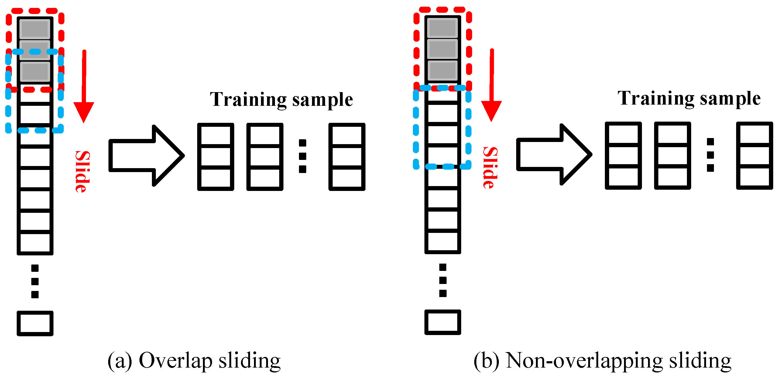
are the minimum and maximum values of the features in the dataset respectively. The input of a deep learning network requires a specific size, so the original training and test sequences are processed using sliding. As shown in
Figure 4a, the overlapping sliding method is used to increase the number of training samples. Assuming the length of the training sequence is
z, a sliding window with a length of
n and a step size of
u (
) is used to slide along the original sequence and obtain
training samples. Similarly, as shown in
Figure 4b, the non-overlapping sliding mode is used for sampling. Assuming the length of the test sequence is
h,
test samples are obtained. Here,
m represents the start of sliding,
n represents the size of the sliding window (i.e., the dimension of the network input), and
represents the start of sliding to the end of the sequence.
In this paper,
,
,
, and
indicators are used for performance evaluation. The mathematical expressions of the three indicators are as follows:
where
is the label data and
is the predicted data. The model was trained by GeForce RTX 2080Ti GPU, equipped with an Intel i5-processor, 64 GB-RAM, and the Ubuntu-system. The model was built based on the Python framework, and the Adam optimizer was used for gradient update.
3.2. Evaluating on AEP Dataset
In order to verify the effectiveness of this method, this paper compares various load forecasting methods, including linear regression (LR), ARMA, BP neural network, SVR, decision tree (DT), CNN, LSTM, Resnet, STLF [
12], ELM [
14], CN-Fuzzy [
22], MB-LSTM [
28], MIFnet [
30], and Transformer [
37]. The above methods include the classic forecasting model and the SOTA load forecasting model recently proposed.
According to the characteristics of the AEP dataset, 23 time series features, such as energy use, T1-T9, RH1-RH9, the temperature outside, pressure, humidity outside, and wind speed were used as the input of the network, and the total predicted load consumption was used as the output. In the comparative experiment, we used the grid search method to fine-tune the hyperparameters of each related method. In addition, some related methods disclosed their optimal hyperparameter settings, and we borrowed the optimal hyperparameter settings of these methods. Due to the large number of input feature dimensions, the importance of the feature is inconsistent. For example, we found that the temperature feature has a greater impact on the results, and the visibility feature has a smaller impact on the prediction results.
Therefore, the assignment of the importance of the feature is particularly important for the accuracy of the prediction results.
Table 1 shows the comparison results between this method and the other 14 methods. These 14 methods include the regression method, traditional machine learning method, and the latest deep learning method for load forecasting. From the four indicators, the method based on deep learning is obviously superior to the regression method and traditional machine learning method. Traditional machine learning methods are prone to over-fitting when facing large sample data, resulting in poor generalization effect, which affects the prediction accuracy. The regression-based method is the worst in MSE and MAE indicators, but it performs better in MAPE indicators. With the two methods, LR and ARMA, the error is large in the area with large load consumption, but the area with load consumption that is close to 0 performs stably, which lowers the overall mean absolute percentage error.
For load forecasting, slight fluctuations in the forecast near the load usage of 0 will lead to a sharp increase in error indicators, but users will not be sensitive to these fluctuations. In general, the accurate prediction of load peaks will be beneficial to users, which is also the role of load forecasting. It can be seen from the results that although the prediction accuracy of the CNN method and LSTM method is better than the traditional machine learning model, the overall accuracy is not high, lower than the improved models CNN-Fuzzy, MB-LSTM and MIFnet. In addition, the Transformer network can effectively process time series data, and the overall performance is due to the existing methods. In order to show the effectiveness of this method more clearly, we conducted ablation experiments. The results show that the MCM structure and DAM module can effectively improve the accuracy of prediction.
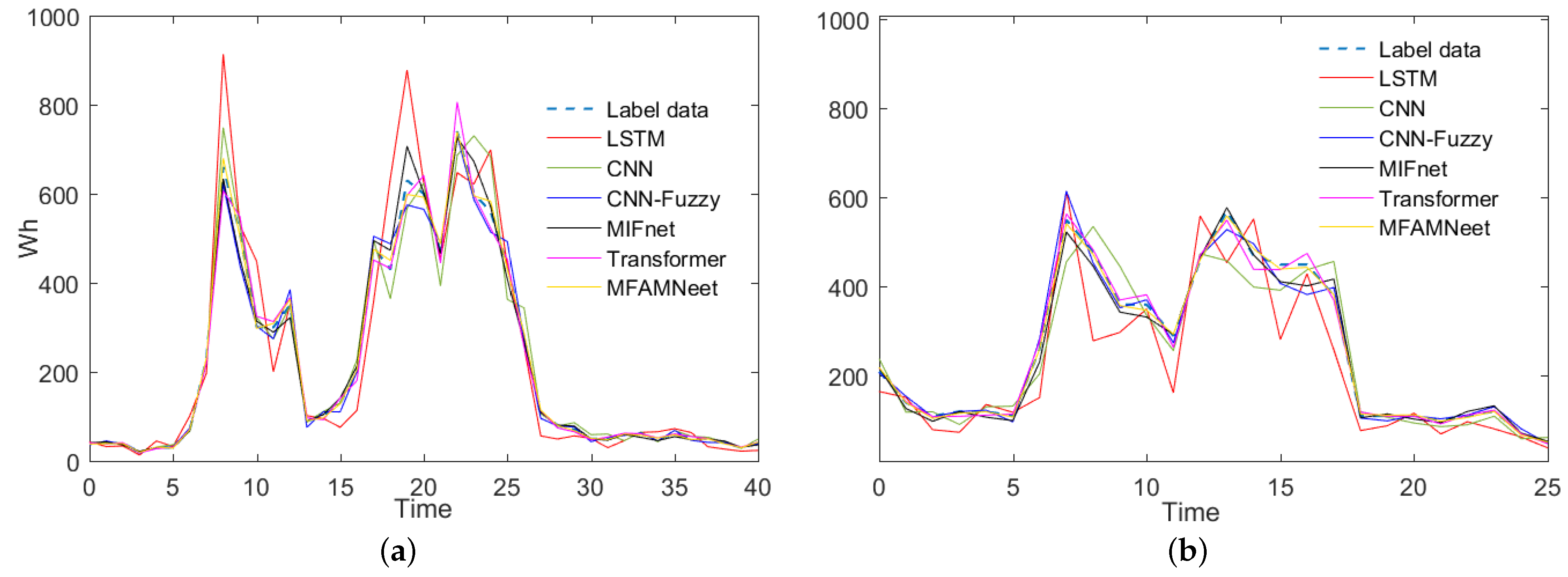
Figure 5 shows the comparison between this method and some deep learning methods. Because the prediction effect of the regression method and traditional machine learning method is not good, these methods are not drawn in the comparison chart. It can be seen from
Figure 5 that the method in this paper fits the load curve very well and has the best effect. This is because this method can achieve multi-scale feature extraction, and can use the channel attention mechanism to assign the importance of 23 features, improving the effectiveness and accuracy of prediction. The LSTM method can effectively extract the temporal correlation, but from the experimental results, it is easy to have a prediction peak, i.e., it is easy to have a higher load prediction at the actual load peak, and the algorithm prediction inertia is large. The prediction accuracy of the CNN method at load change is not high. The existing improved methods CNN-Fuzzy and MIFnet have significantly improved compared with LSTM and CNN.
Figure 6 shows the comparison of ablation experiments. From the results of the ablation experiments, it can be seen that the prediction accuracy of the two-branch attention mechanism model at the time series mutation is better than that of the network without the attention mechanism. As can be seen from
Figure 6, when there is no attention mechanism, the prediction results fluctuate greatly and the prediction inertia is large, resulting in the prediction results at the wave peak often being larger than the actual values. In addition, the multi-scale convolution module can effectively improve the accuracy of model prediction.
3.3. Evaluating on IHEPC Dataset
In this paper, the features of global_active_power, global_reactive_power, voltage, global_intensity, sub_metering_1, sub_metering_2, and sub_metering_3 in the IHEPC dataset are used as the input feature and predict the future active power.
Table 2 shows the comparison results between the proposed MFAMNet method and the other 14 methods. It can be seen from
Table 2 that the MFAMNet method proposed in this paper is obviously superior to the existing methods. Compared with
Table 1, the MSE, MAE, and RMSE indicators in
Table 2 are significantly reduced. This is due to the frequent use of load in AEP datasets and the low power consumption in most time intervals in IHEPC datasets, which lowers the MSE, MAE, and RMSE indicators. Similarly, since the power consumption of most time areas of the IHEPC dataset is very small, the MAPE index of LR, ARMA is improved. In addition, from the perspective of ablation implementation, the two modules proposed in this paper greatly improve the prediction accuracy of the model.
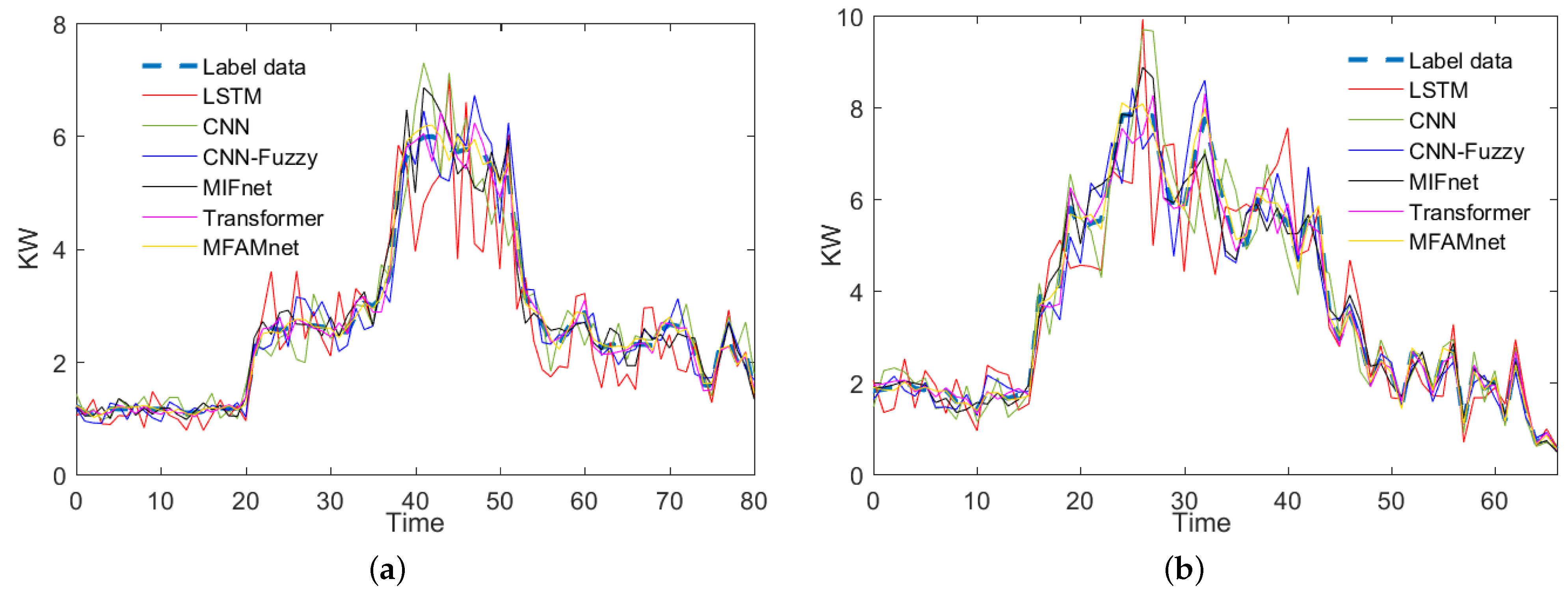
Figure 7 shows the prediction comparison between the method in this paper and the existing methods. It can be seen from the results that the differences between the method in this paper and the label data are very small. LSTM is highly volatile. Although LSTM can extract temporal features, its ability to express multi-dimensional features is limited. Several improved deep learning networks performed well and can make up for the shortcomings of traditional deep learning methods. The Transformer model is built based on attention, so it improves the feature expression ability of the network to a certain extent. In general, the MFAMNet method proposed in this paper can effectively predict the peak load, and the effect is due to all other methods.


