JAUNet: A U-Shape Network with Jump Attention for Semantic Segmentation of Road Scenes

Abstract

The task of complex scene semantic segmentation is to classify and label the scene image pixel by pixel. For the complex image information in autonomous driving scenes, its characteristics such as many kinds of targets and various scene changes make the segmentation task more difficult, making various kinds of FCN-based networks unable to restore the image information well. In contrast, the encoder–decoder network structure represented by SegNet and UNet uses jump connections and other methods to restore image information. Still, its extraction of shallow details is simple and unfocused. In this paper, we propose a U-shaped convolutional neural network with a jump attention mechanism, which is an improved encoder plus decoder structure to achieve semantic segmentation by four times of convolutional downsampling and four transposed convolutional upsamplings while adding a jump attention module in the upsampling process to realize selective extraction of contextual information from high-dimensional features to guide low-dimensional features, improve the fusion of deep and shallow features, and ensure the consistency of the same type of pixel prediction. The CamVid and Cityscapes datasets are sampled for the experiments, and the model ground mIoU evaluation metrics can reach 66.3% and 69.1%. Compared with other mainstream semantic segmentation algorithms, this method is competitive in terms of segmentation performance and model size.

1. Introduction

Image semantic segmentation techniques are widely used in artificial parsing, virtual reality, self-driving cars and other fields. According to relevant statistics, by the end of 2020, only 10% of the 1 billion cars in use worldwide will have installed advanced driver assistance systems (ADAS) features. Therefore, autonomous driving technology has a wide market and a strong development prospect. Among the many technologies of autonomous driving, the detection of the surrounding environment in the process of vehicle driving is the basis for achieving intelligent vehicle driving. With the rapid development of convolutional neural networks (CNNs), a fully convolutional network (FCN) method is gradually replacing the traditional image segmentation method. Because of its hierarchical feature extraction and implementation of an end-to-end training structure, many later full convolutional neural network-based approaches have achieved satisfactory results in pixel-level semantic segmentation tasks.

Classical road detection methods focus on extracting texture and edge information from images. The most basic texture extraction method is the Gabor filter [1]. Gabor features are more sensitive to edges, can extract the direction of edges, are less affected by illumination, and have scale invariance, which can be used to distinguish roads from other different areas. In addition, for road targets with obvious edge demarcation, extracting the edge demarcation of these roads can segment the road surface, and the commonly used edge detection operators are Sobel, Prewitt, and other operators. After calculating the texture or edge features of the road, threshold segmentation can be used to obtain the road segmentation results. In addition, support vector machines and other methods can be used to achieve better segmentation results. Since parallel straight lines exist at the edges of standard roadways, the intersection points of multiple pairs of parallel straight lines (road edge lines and lane lines) can be extracted, and the center positions of these intersection points can be obtained to approximate the extinction points to segment the roadway from other scenes.

With the rapid development of convolutional neural networks (CNNs) [2,3], their excellent hierarchical feature extraction capabilities and end-to-end training structure have led to significant advances in CNNs for pixel-level semantic segmentation tasks as well [4,5]. Long et al. proposed fully convolutional neural networks (FCN) in 2014 [6]. In the FCN model, the fully-connected layer used for classification is changed to a convolutional layer, followed by upsampling of the feature maps using transposed convolution [7]. Finally, a series of classification output maps equal in size to the original image are output, and the maximum value is taken as the prediction class after passing through the Softmax layer. In this way, the FCN model can classify images at the pixel level and complete the semantic segmentation task. The FCN method has achieved superior results in semantic segmentation tasks after its emergence due to its superior results and end-to-end training structure, which, in turn, gradually replaced the traditional image segmentation methods. Wang et al. also used FCN’s decoder network for tasks such as optimizing transmission systems [8]. In the following years, to solve the problem of special detection learning for multi-scale targets, Chen et al. designed the Deeplab network architecture [4,9]. Its multi-scale feature extraction is achieved by using different null convolutions (atrous conv). PSPNet [10] designed a spatial pyramid pooling (SPP) structure to pool different size targets onto the same feature space. MLNet [11] and MANet [12] also use multi-scale feature fusion models to optimize image segmentation tasks. Song et al. also involved a two-branch network model for image segmentation [13]. These network architectures can optimize the semantic segmentation effect very well, but a large amount of computation and a complex network structure also become the disadvantages of such methods.

As the network layer deepens, the feature map resolution decreases and contains less spatial detail information, and the reconstruction of the resolution has to be carried out before obtaining the segmentation results. It is difficult for the ordinary FCN network to restore the spatial detail information of the image better, which becomes another difficulty in the semantic segmentation task. Some U-shape structures (i.e., encoder–decoder structures) can better restore the spatial information of images, such as the UNet structure proposed by Ronneberger et al. [14] and the SegNet structure extracted by Badrinarayanan et al. [15]. Such structures use low-level information to assist higher-level features in recovering image details through an encoder–decoder structure. However, this type of network structure also has certain drawbacks. SegNet only passes the pooling index of the lower layer to the higher layer for upsampling while UNet directly superimposes the lower layer features onto the higher layer features without more processing, which may lead to inconsistent segmentation results of the network for the same target. Networks that also use encoder–decoder structures, such as GCN [16] and DDSC [17], have chosen to use more complex decoder structures to enhance the segmentation, but this also increases the complexity of the network.

Combined with the above methods, although the traditional road segmentation methods are simple to calculate and have fair results, the color and texture information cannot further help us segment the image in the face of the complex road scenes in the actual driving process. In contrast, methods based on image filtering, graph theory, or clustering cannot extract further image features, and the segmentation accuracy does not meet the demand well. In addition, because of the high segmentation requirements for off-road targets in today’s autonomous driving scenarios, as well as the need to obtain the class to which each segment belongs, traditional methods are no longer adequate for today’s autonomous driving scenarios. For FCN and Deeplab, although better segmentation results can be obtained, the network structure is more complex, and the deep network ignores the shallow feature information, so the final segmentation results are blurred at the edge contour. Although SegNet and UNet fuse the low-level features with the high-level features, they do not process the low-level features, which may bring a lot of useless information to the high-level features and affect the final segmentation results. In order to solve the problem of combining low-level features and high-level features, this paper draws on attention mechanisms such as SE-Net [18] and CBAM [19], which are improved based on UNet and GAU structures [20], and use high-level features to generate channel attention weights to assist low-level features for feature extraction. We also add the ConvLSTM module [21] for extracting temporal contextual information between images to obtain better segmentation results.

2. Materials and Methods

The overall framework of the model is shown in Figure 1, which is divided into 2 processes, encoding and decoding, where the input image is extracted with different levels of features through the underlying network in the encoder. Then it arrives at the ConvLSTM module for temporal information extraction, and subsequently enters the decoder section for upsampling and feature fusion through the jump attention module to finally obtain the prediction results. The encoder in the network uses VGG16 [22] as the base network structure, using a 3 × 3 convolution, a batch normalization and a relu activation for each downsampling, and, finally, a maximum pooling operation to reduce the feature map size to 1/4 of the original. In this paper, the fully connected layer of VGG16 is removed, which makes the JAUNet encoder network smaller and easier to train than many other recent architectures [23,24]. After going through four times of downsampling, the number of feature map channels is 1024 and the length and width of the feature map is 1/16 of the input image. In addition, in the upsampling process, the feature map size is scaled up to twice at the time, using transposed convolution, followed by connecting the lower-level features that have been processed with jump attention. After convolutional normalization, the next upsampling is performed, and the image is restored to its original size after four upsamplings, and the number of channels is the predicted number of classes N.

2.1. UNet Network Structure

UNet was originally designed to be used for the task of semantic segmentation of medical images. Ronneberger designed this network in 2015 and won the ISBI Cell Tracking Challenge that year by a huge margin with the network structure shown in Figure 2. UNet is a convolutional neural network based on the basic network structure of FCN, which uses an encoder–decoder structure. The encoder part of UNet adopts a 4 convolutional downsampling structure, and the decoder part adopts a 4-transposition convolutional upsampling structure. In addition, the shallow features in the downsampling process are combined with the deep features in the upsampling process using a jump connection, so that the deep features can be used for localization and the shallow features can be used for accurate segmentation of the image. After the encoder–decoder structure, the last convolutional layer is used for the output, and the output feature map size is the same as the input image size and the number of channels is the same as the desired number of classifications, and the final segmentation result can be calculated after passing Softmax.

2.2. Convolutional LSTM (ConvLSTM) Network Structure

The Convolutional LSTM (ConvLSTM) [21] network structure changes the input to an M × N grid with P number of channels per grid compared to the traditional LSTM network, so the input to the network is a 3D tensor. The authors of this paper also gave the formula for the ConvLSTM structure, as in Equation (1).

$$\begin{gathered} i_t=\sigma \left(W_{xi}\ast X_t+W_{hi}\ast H_{t-1}+W_{ci}\circ C_{t-1}+b_i\right) \\ {f}_t=\sigma \left(W_{xf}\ast X_t+W_{hf}\ast H_{t-1}+W_{cf}\circ C_{t-1}+b_f\right) \\ {C}_t=f_t\circ c_{t-1}+i_t\circ \tanh \left(W_{xc}\ast X_t+W_{gc}\ast H_{t-1}+b_c\right) \\ {o}_t=\sigma \left(W_{xo}\ast X_t+W_{ho}\ast H_{t-1}+W_{co}\circ C_t+b_o\right) \\ {C}_t=o_t\circ tanh\left(C_t\right) \end{gathered}$$

(1)

In the formula, the asterisk represents the convolution operation. ConvLSTM combines the advantages of convolutional neural networks and recurrent neural networks, which makes it suitable for spatio-temporal data and can be used in video ground semantic segmentation tasks. Its structure is shown in Figure 3.

2.3. Jump Attention Module (JAM)

In deep learning application scenarios, we often need to deal with exceptionally large amounts of data, but only a small fraction of most of the data is important, and attention mechanisms are used for extracting the highlights from large amounts of data in deep learning tasks. In image processing, the attention mechanism can also play a good role, mainly by further feature extraction of the feature map, calculating the attention weights on the image channel or space, and re-acting on the original feature map to selectively extract image information. This has been previously used by networks such as SE-Net [18] and CBAM [19]. In this case, SE-Net first performs a Squeeze operation on the feature map, which uses global pooling to synthesize the input features of size 2C × H × W into a C × 1 × 1 feature description. After the above Squeeze operation, the network only gets a global description, which cannot be used as the weight of the channel. Therefore, the authors proposed the Excitation operation, which contains two fully connected layers, and the Sigmoid activation function, to obtain the channel attention weights for processing the original feature map. Attention mechanisms are also often used in the field of weather image segmentation [25,26,27]. We design the jump attention module to address the problem that the commonly used U-shaped network structure does not further process the low-dimensional features during the jump connection process, considering that the high-dimensional features have rich semantic information, which can help guide the selection of low-dimensional information, so as to achieve the selection of more accurate resolution information, and, finally, combine the processed feature maps to the high-level features for upsampling operations. Its structure is shown in Figure 4.

As shown in the figure, the attention structure in this paper utilizes both high-dimensional features and low-dimensional features as a way to compensate for the UNet network’s lack of any processing of low-level jump connections afterwards. The feature map size of the upsampling process is 2C × H × W, which is converted to C × 1 × 1 channel attention weights after a series of pooling and feature extraction, and feature fusion processing with low-dimensional features of size C × 2H × 2W. The method is to first convolve the low-dimensional features by 3 × 3, followed by matrix multiplication with the channel attention weights extracted from the high-dimensional features to obtain the attention-processed feature map for subsequent upsampling with the high-dimensional feature evaluation for the next step. The formula for the jump attention module is given in Equation (2).

$$M_c\left(L\right)=M_c\left(H\right)\times Con{v}_{3\times 3}\left(L\right)$$

(2)

In the formula, $M_c\left(H\right)$ represents the attention weight calculated from the high−dimensional feature map. $Con{v}_{3\times 3}$ represents the 3 × 3 convolutions, $L$ represents the low−dimensional feature map, and $M_c\left(L\right)$ represents the feature map after JAM processing.

Adding the attention mechanism on image channels was proposed in 2018 by Hu et al.’s SE-Net model [18]. This paper adds a parallel maximum pooling layer compared to the channel attention mechanism in SE-Net. A three-layer perceptron is also used, instead of the original 1 × 1 convolution, to extract the channel attention information, and, finally, the channel attention weights with the same number of channels and low-dimensional features are output. The structure of the channel attention mechanism designed in this paper is shown in Figure 5.

The channel attention mechanism computes the maximum pooling and average pooling of the input features and feeds them to the $MLP$ unit, a two-layer neural network for computing the attention weights on the picture channels. The formula for the channel attention mechanism is given in Equation (3).

$$\begin{gathered} M_c\left(H\right)=\sigma \left(Conv\left(MLP\left(AvgPool\left(H\right)\right)+MLP\left(MaxPool\left(H\right)\right)\right)\right) \\ =\sigma \left(Conv(W_1\left(W_0\left(H_{avg}^c\right)\right)+W_1\left(W_0\left(H_{max}^c\right)\right)\right)) \end{gathered}$$

(3)

According to Equation (4), the number of feature vector channels is reduced by half after passing the last convolution layer. Input high-dimensional features of size 2C × H × W for the high-level features, generating C × 1 × 1 attention weights with the same number of channels as the low-dimensional features. Finally, after passing the low-level channels through a 3 × 3 convolutional layer, the attention-processed feature map is obtained by multiplying it with the attention weights, calculated as in Equation (4).

$$M_c\left(L\right)=\sigma \left(Conv(W_1\left(W_0\left(H_{avg}^c\right)\right)+W_1\left(W_0\left(H_{max}^c\right)\right)\right))\times Con{v}_{3\times 3}\left(L\right)$$

(4)

At this point, the size of the generated jump feature map is C × 2H × 2W, which is the same size as the high-dimensional features after one upsampling, and the low-dimensional features and high-dimensional features after channel attention processing are stitched together to obtain the feature map obtained from this round of upsampling and the feature map used in the next round of upsampling, as in Equation (5).

$$H_{next}=Upsample\left(H\right)+M_c\left(L\right)$$

(5)

In summary, the output feature map of the attention module in this paper has exactly the same size and number of channels as the low-level feature map, and there are not too many weights, so it can be easily added to the existing network and can effectively extract the picture ground channel and spatial attention information, which can well save hardware resources.

3. Results

3.1. Benchmark Dataset

3.1.1. CamVid Dataset

Semantic segmentation models based on deep learning require a large number of datasets for model training, and the datasets used vary in the face of different semantic segmentation tasks; for instance, in the semantic segmentation task of medical images, 3D medical image datasets are often used. The CamVid dataset [28] can be used to meet the needs of this paper, which requires time series images or video datasets. This is an RGB street view dataset developed and labeled by the University of Cambridge. The CamVid raw dataset contains a total of 701 photos with a resolution of 720 × 960, containing a total of 32 raw categories that can be grouped into 11 major categories, including vehicles, pedestrians, roads, and buildings. The dataset, consisting of a series of sequential images, was taken under different lighting conditions and was taken while the car was in motion, which is well suited to the environment of autonomous driving use. It can meet the dataset needs of this paper. We followed the official CamVid data divisions of training set, validation set, and test set. The number of images in the training set, validation set, and test set are 367, 101 and 233, respectively. Figure 6 shows an example of the comparison between the original image and the labeled image.

3.1.2. Cityscapes Dataset

The Cityscapes dataset [29] is a large cityscape dataset that contains high-resolution images of driving scenes taken in more than fifty different cities, in different contexts and in different seasons. It includes three seasons of street scenes in spring, summer and autumn, and uses a binocular camera to obtain a stereoscopic video sequence. The dataset has a large number of well-labeled street images, including 5000 finely labeled images and 20,000 coarsely labeled images with resolutions up to 1024 × 2048. The Cityscapes dataset does not supply data labels for the Test set. Therefore, we have re-segmented the training and validation sets for a total of 3475 images. The dataset was generated in the ratio of 6:2:2 for the training, validation, and test sets. The Cityscapes dataset is labeled with 19 different categories, and the correspondence between the original images and the classification labels is shown in Figure 7.

3.2. Experimental Platform and Environment

The CPU used for the experiments is INTEL CORE I7-12700 (INTEL, Santa Clara, CA, USA, with 32 GByte of memory), the GPU used for the experiments is NVIDIA Geforce RTX3070 (NVIDIA, Santa Clara, CA, USA, with 8 GByte of memory), and the software is Pytorch, a deep learning framework. Data is processed using the Numpy library and visualised using libraries such as PIL and Plotly. Detailed hardware and software parameters are shown in

Table 1. Experimental hardware model.

Hardware	Manufacturer	Model
CPU	INTEL, Santa Clara, CA, USA	Core i7-12700
GPU	NVIDIA, Santa Clara, CA, USA	Geforce RTX3070
Memory	G. SKILL, Taipei, Taiwan, China	F4-3200C16D 8 GB × 4
SSD	Samsung, Yongin, Gyeonggi-do, Korea	980pro 1TB

and

Table 2. Experimental software and version.

Software	Version
Windows 11	22H2
Conda	4.13.0
Python	3.9.12
Pytorch	1.12.0
Cudatoolkit	11.3.1
Matplotlib	3.5.1
Numpy	1.22.3

.

The experiments use the small batch stochastic gradient descent (SGD) method with a momentum setting of 0.9 and a weight decay of 10⁻², using “poly” as the learning rate decay strategy, where the initial learning rate is set to 0.05 and the exponential coefficient is 0.9. During the training process, the max epoch is set to 200. In the Cityscapes dataset, the resolution of the images was randomly cropped to 512 × 1024 during the training phase in order to make a fair comparison with different semantic segmentation network models; For the CamVid dataset, experiments were conducted using a resolution of 360 × 480. It should be noted that the new network model proposed in this paper does not use pre-training operations.

3.3. Evaluation Indicators

The $PA$ represents the proportion of correctly classified pixels to all pixels and is calculated as in Equation (6).

$$PA=\frac{{{\displaystyle \sum }}_{i=1}^k{p}_{ii}}{{{\displaystyle \sum }}_{i=0}^k{{\displaystyle \sum }}_{j=0}^k{p}_{ij}}$$

(6)

where $k$ denotes that there are $k$ classes of all pixel points, $p_{ij}$ denotes the number of pixel points in class $i$ that are predicted as class $j$, and $p_{ii}$ denotes the number of pixel points in class $i$ that are correctly predicted as class $i$. In the confusion matrix, $p_{ij}$ can be found in the $i$-th column and $j$-th row, and $p_{ii}$ in the same way. Therefore, after calculating the confusion matrix, we can easily calculate the pixel classification accuracy.

$MPA$ is a boost to $PA$, which is calculated by figuring out the proportion of correctly classified pixel points of each class to the pixel points of the whole class, and then calculating the average value of pixel classification accuracy for all classes, which is calculated as in Equation (7).

$$MPA=\frac{1}{k+1}{\displaystyle \sum }_{i=0}^k\frac{p_{ii}}{{{\displaystyle \sum }}_{j=0}^k{p}_{ij}}$$

(7)

As the name suggests, $IoU$ represents the ratio of the intersection of the target region and the predicted region to the concurrent set, expressing the overlap between the target region and the predicted region, and the higher the intersection ratio indicates, the higher the accuracy of the segmentation is, as calculated in Equation (8).

$$IoU=\frac{p_{ii}}{{{\displaystyle \sum }}_{j=1}^k{p}_{ij}+{{\displaystyle \sum }}_{j=1}^k{p}_{ji}-p_{ii}}$$

(8)

Like $IoU$, $MIoU$ is also the ratio of the intersection of the target region and the predicted region to the concatenated set, which is calculated for each pixel category and then for the average value of the intersection ratio for all categories. The higher the value indicates, the higher the accuracy of the segmentation is, and the formula is as in Equation (9).

$$MIoU=\frac{1}{k+1}{{\displaystyle \sum }}_{i=0}^{k}IoU$$

(9)

$FWIoU$ is a boost for $MIoU$. This method uses the frequency of occurrence of each class as a weight to calculate the mean value of IoU, which can better represent the accuracy of semantic segmentation, which is calculated as in Equation (10).

$$FWIoU=\frac{1}{{{\displaystyle \sum }}_{i=0}^k{{\displaystyle \sum }}_{j=0}^k{p}_{ij}}{{\displaystyle \sum }}_{i=0}^{ak}\frac{p_{ii}}{{{\displaystyle \sum }}_{j=1}^k{p}_{ij}+{{\displaystyle \sum }}_{j=1}^k{p}_{ji}-p_{ii}}$$

(10)

3.4. Loss Function

The basic loss function used in this paper is the NLLLoss loss function provided by Pytorch, which can be used with the Softmax function to achieve the need for fast descent in the case of high error and close to the optimal solution. The optimal solution of the model turns to be better and faster. Since the experimental dataset belongs to the complex scene segmentation dataset, the samples have the characteristics of containing many target categories and an unbalanced number, which leads to the fact that the model cannot learn the features of each category equally and guarantee the segmentation accuracy of each category. In this paper, the category balance method is used to calculate the occurrence frequency $f{q}_i$ of each category, which is the number of pixels in that category divided by the total number of pixels in the data, where $i$ represents the i-th category. In addition, the median value of the occurrence frequency $f{q}_s$ of all categories is found and divided by the corresponding frequency of that category to obtain the weight of that category, which is calculated as in Equation (11).

$$weigh{t}_i=median\left(f{q}_s\right)/f{q}_i$$

(11)

The generated category weights are used to act on the loss function to make it more sensitive to the categories that occur less frequently, and the formula of the loss function after increasing the weights is shown in Equation (12).

$$Loss=-{\displaystyle \sum }_{i=1}^N{w}_{i}NLLoss\left(y_i,p_i\right)$$

(12)

The $w_i$ in the formula is the weight of class $i$; $y_i$ and $p_i$ are the label values and predicted values of all class $i$ in the image respectively.

Also, this paper introduces the Dice Loss function as an auxiliary loss function, which is a loss value calculated from the Dice coefficient, an ensemble similarity measure function usually used to calculate the similarity of two sample points with the formula in Equation (13).

$$S=\frac{2\left|X\cap Y\right|}{\left|X\right|+\left|Y\right|}$$

(13)

where $\left|X\cap Y\right|$ denotes the intersection between $X$ and $Y$; $\left|X\right|$ and$\left|Y\right|$ denote the number of elements of $X$ and $Y$, respectively. The factor 2 in the numerator is due to the existence of double counting the common elements between $X$ and $Y$ in the denominator. If the Dice coefficient is larger, it indicates that the more similar the set is, the smaller the Loss is; and vice versa. Therefore, the Dice Loss is calculated as in Equation (14).

$$DiceLoss=1-\frac{2\left|X\cap Y\right|}{\left|X\right|+\left|Y\right|}$$

(14)

$\left|X\cap Y\right|$ denotes the dot product of the corresponding elements of two sets and then sums the results of the element-by-element multiplication.

Dice Loss and NLLLoss are often used together and in this paper, they are weighted as the overall Loss, calculated as in Equation (15).

$$Final Loss=\alpha \times NLLLoss+\beta \times DiceLoss$$

(15)

FCN-ResNet18 was used in advance as the base model to test both weights on the CamVid dataset, and each combination of weights was trained with 100 epochs. Finally, the test set mIoU was calculated to evaluate the training effect of each weight. The test results are shown in

Table 3. Effect of different weight loss functions on segmentation performance. The bolded part indicates the best performance of each indicator at this parameter.

$\mathit{\alpha }$	$\mathit{\beta }$	PA	MPA	FWIoU
1	0	80.7	64.4	72.3
0.8	0.2	82.5	64.2	74.0
0.6	0.4	83.0	63.1	74.2
0.4	0.6	79.3	64.2	70.5
0.2	0.8	77.3	64.5	69.4

. Since it is unfavorable to small samples when using DiceLoss completely, the cases of $\alpha =0$ and $\beta =1$ are not considered.

It can be seen that the test set performs best when $\alpha$ is taken as 0.6 and $\beta$ is taken as 0.4, so this combination of weights is chosen as the weights for subsequent experiments.

The gradient descent algorithm used in this paper is stochastic gradient descent (SGD). This gradient descent algorithm can sample a portion of the training set data, which is a mini-batch. This parameter can be set by itself. After the forward propagation of the network is completed, SGD gradient descent then uses the loss function calculated from this batch of the training set to calculate the optimal value of the weights until the model converges or the algorithm is stopped manually. SGD has been shown to have better performance in various experiments [30].

3.5. Experimental Evaluation

In this section, the actual segmentation performance of the trained networks on the two datasets will be presented. The segmentation images generated by each network will be presented for evaluating the visual segmentation effect, and the objective evaluation metrics calculated for comparing the segmentation effect of each network will also be presented.

3.5.1. Ablation Experiments

We conducted ablation experiments on the CamVid dataset for both the JAM module and the ConvLSTM module. We tested combinations of different numbers of JAM modules and ConvLSTM modules. The test results are shown in

Table 4. Results of ablation experiments for JAM module and ConvLSTM module. The bolded part indicates the best performance of each indicator at this parameter.

Network	Speed/fps	Params/M	MIoU	FWIoU
UNet [14]	39.51	7.76	63.7	72.6
UNet + ConvLSTM	25.39	26.58	64.1	70.1
UNet + 1 × JAM	38.95	9.34	63.9	72.5
UNet + 2 × JAM	37.60	11.22	64.5	72.1
UNet + 3 × JAM	36.34	15.31	65.5	73.1
UNet + 4 × JAM	31.22	18.50	65.3	72.8
UNet + 3 × JAM + ConvLSTM	35.23	33.91	66.3	74.2

.

Table 4 shows that the ConvLSTM module alone does not improve the MIoU much, and the effect even decreases in the metric FWIoU. In contrast, the JAM module alone has a significant improvement on both MIoU and FWIoU for the native UNet network. The segmentation accuracy of the UNet network gradually improves as more JAM modules are used. However, when we added JAM modules at the bottom layer of the network, the effect was not obvious and even degraded in the evaluation metrics, so our final network structure used only three JAM modules. In addition, after using three JAM modules and the ConvLSTM module, the JAUNet network shows a significant improvement compared with the base UNet network, which proves the good cooperation between the ConvLSTM and JAM modules.

3.5.2. CamVid Dataset Results

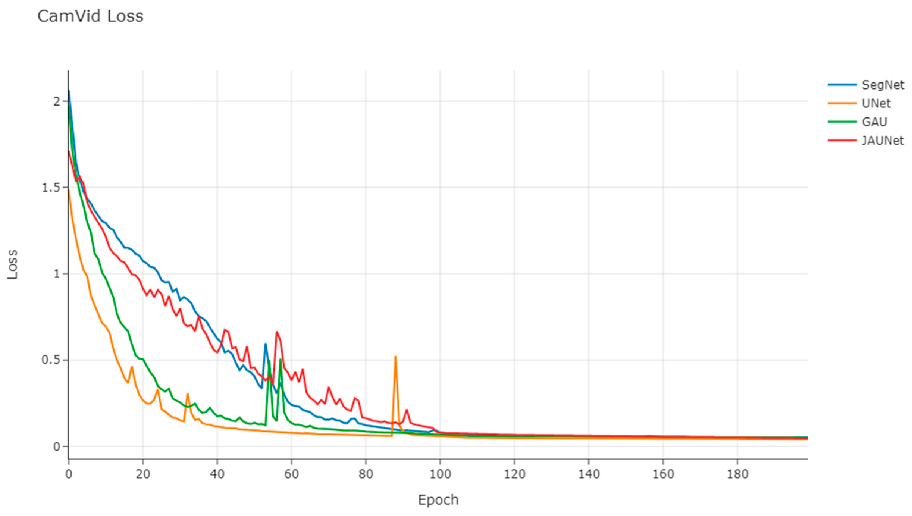
We tested some networks to compare with JAUNet, and Figure 8 gives the change process of the loss function during the training of some networks.

As shown in the figure, the losses of each network gradually converge after 100 rounds of training, and finally they all stabilize at about 0.04. Among them, UNet converges faster, while SegNet and JAUNet converge slightly slower.

The objective evaluation metrics of the four models on the CamVid dataset are shown in

Table 5. Evaluation metrics for each model on the CamVid dataset.

Network	Input Size	Speed/fps	Params/M	MIoU	FWIoU	GFLOPs
ALE [31]	360 × 480	-	-	53.6	62.1	-
SuperParsing [32]	360 × 480	-	-	42.0	52.0	-
FCN-ResNet34	360 × 480	157.10	21.34	49.1	60.5	55.89
ENet [33]	360 × 480	135.4	0.37	51.3	63.2	3.83
SegNet [15]	360 × 480	46.18	29.45	55.6	66.9	104.54
ESPNet [34]	360 × 480	132.00	0.36	55.6	67.2	3.31
PSPNet-ResNet18	360 × 480	25.98	46.64	57.1	68.8	123.69
GAU [20]	360 × 480	38.15	7.94	64.5	72.3	81.64
DeepLab-LFOV [4]	360 × 480	122.53	15.31	61.6	69.3	125.00
ICNet [35]	360 × 480	27.8	26.5	67.1	74.5	28.3
DFANet A [36]	360 × 480	120	7.8	64.7	72.8	3.4
DFANet B [36]	360 × 480	160	4.8	59.3	69.0	2.1
BiSeNetV1_X [37]	720 × 960	175.00	49.00	65.6	73.1	8.70
BiSeNetV1_R [37]	720 × 960	116.30	5.8	68.7	75.9	32.4
JAUNet	360 × 480	35.23	33.91	66.3	74.2	137.76

.

As shown in Table 5, compared with other types of network structures, JAUNet has advantages over most other network structures with a fixed input size of 360 × 480. Compared with the basic semantic segmentation network structure of FCN, JAUNet also achieves excellent segmentation results owing to the encoder–decoder network structure. Compared with SegNet and UNet, which are also encoder–decoder networks, the segmentation accuracy of JAUNet is significantly improved, and its edge segmentation results for small targets are even better due to the cross-channel feature fusion mechanism of JAM. Compared with small networks such as ENet and ESPNet, JAUNet has significantly better segmentation accuracy, although it is inferior to such networks in terms of inference speed and model complexity. Compared with DeepLab, which uses the same basic network structure, JAUNet also has an obvious advantage in segmentation accuracy. Compared with ICNet and DFANet, which are newer networks, JAUNet is more balanced in terms of accuracy and speed. For a large network structure such as PSPNet, JAUNet not only has an advantage in segmentation accuracy but also has a certain advantage in inference speed. Meanwhile, compared with BiSeNetV1 with an input size of 720 × 960, JAUNet is slightly inferior to its segmentation results based on ResNet18 due to its inference speed and segmentation accuracy after using Xception39 or ResNet18 as the backbone network and pre-training on ImageNet, but because it needs to perform pre-training, JAUNet is slightly inferior to its segmentation results based on ResNet18. However, since JAUNet needs to perform pre-training, the computational cost is higher, and its model parametric number is also larger (up to 49 M) compared to other network models. JAUNet can achieve better segmentation accuracy with smaller input images than BiSeNet. 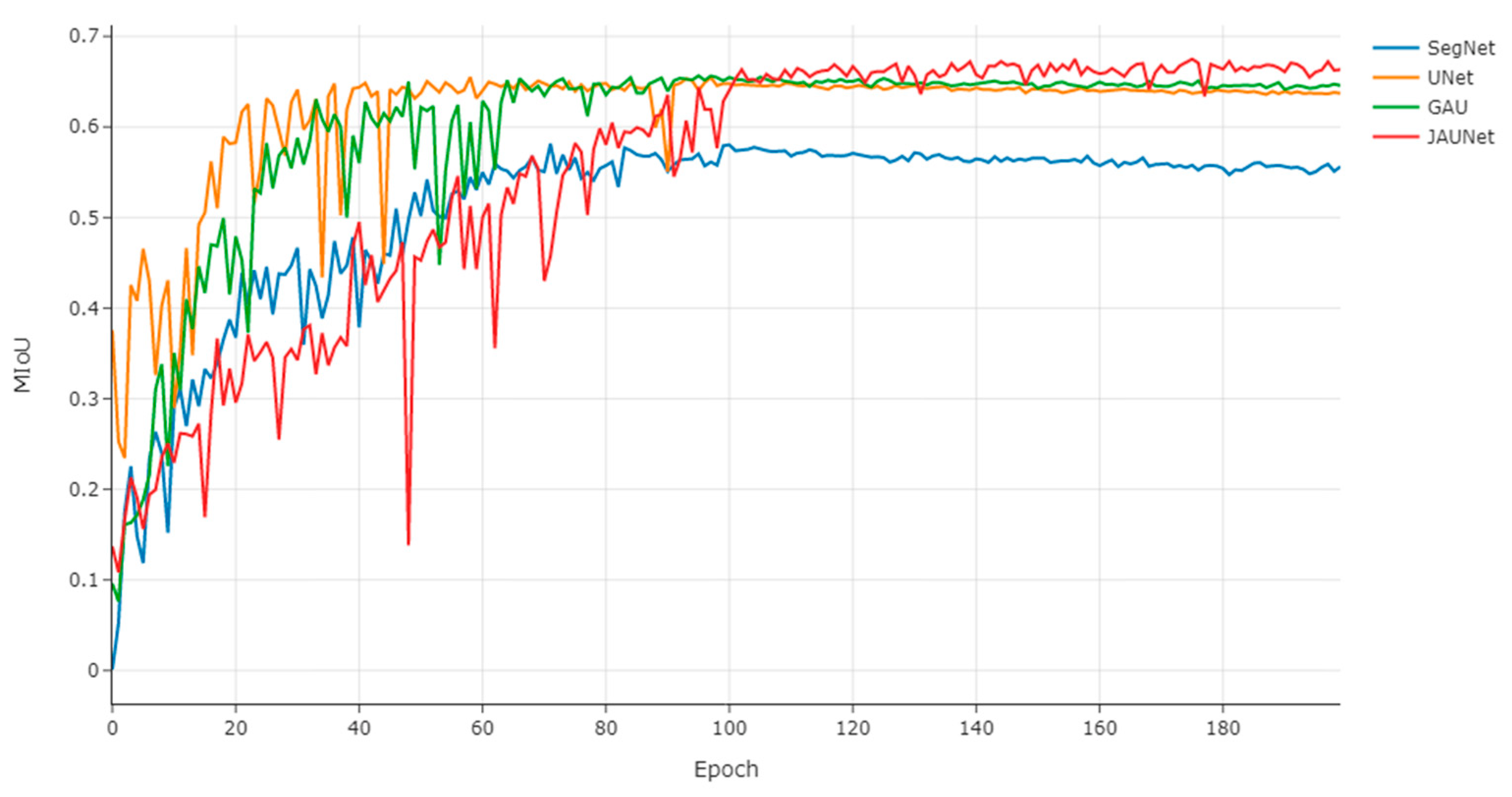Figure 9 also shows the variation of the test machine accuracy with the number of training rounds during training.

Similar to the change of loss function during the training process, the mIoU of JAUNet on the test set rises slowly with the number of training rounds and stabilizes after 100 epochs. According to the change curve of mIoU, it can be found that JAUNet has a significant accuracy advantage on the test set compared to other U-shaped networks by virtue of the JAM attention module, which demonstrates the effectiveness of the JAM module.

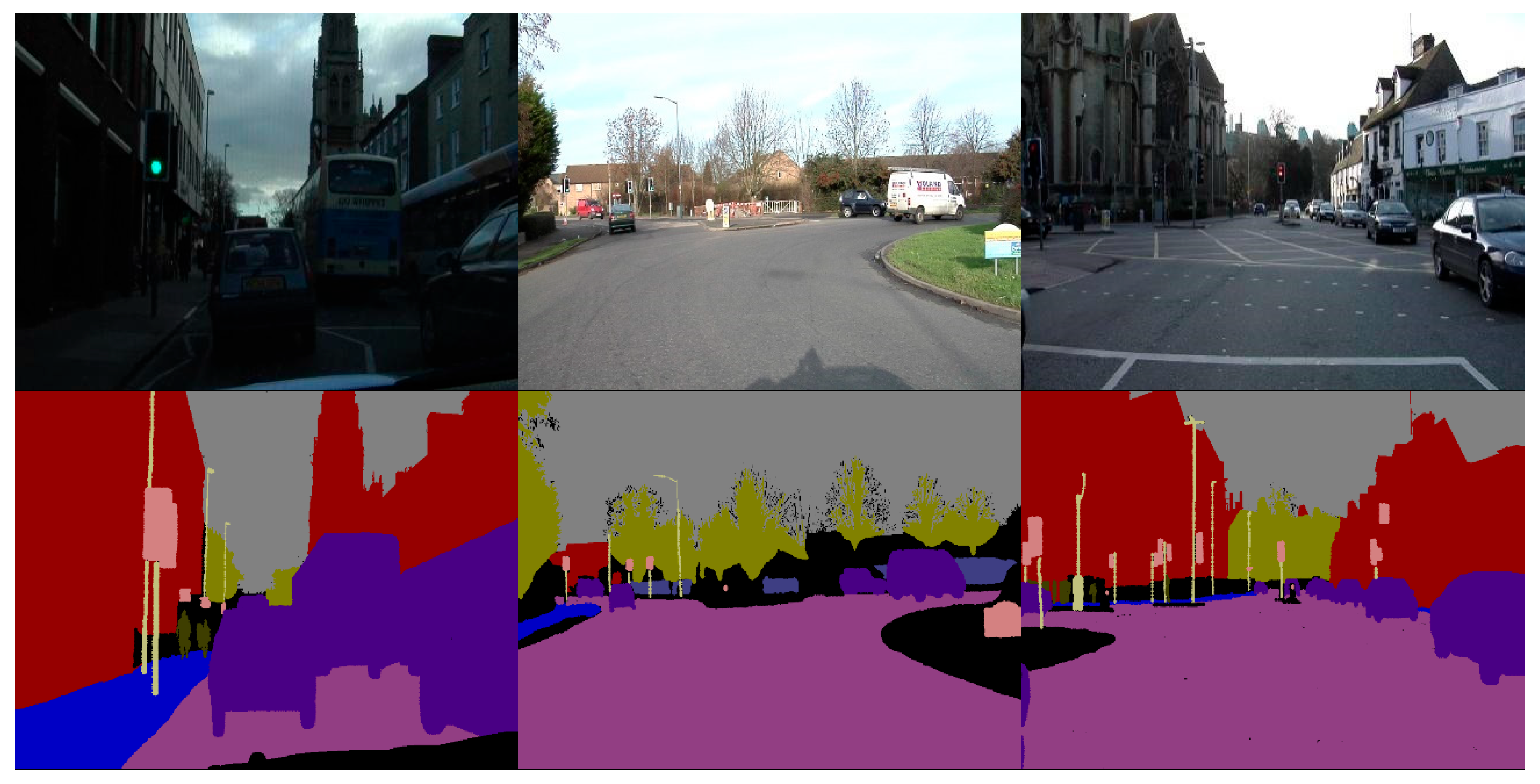
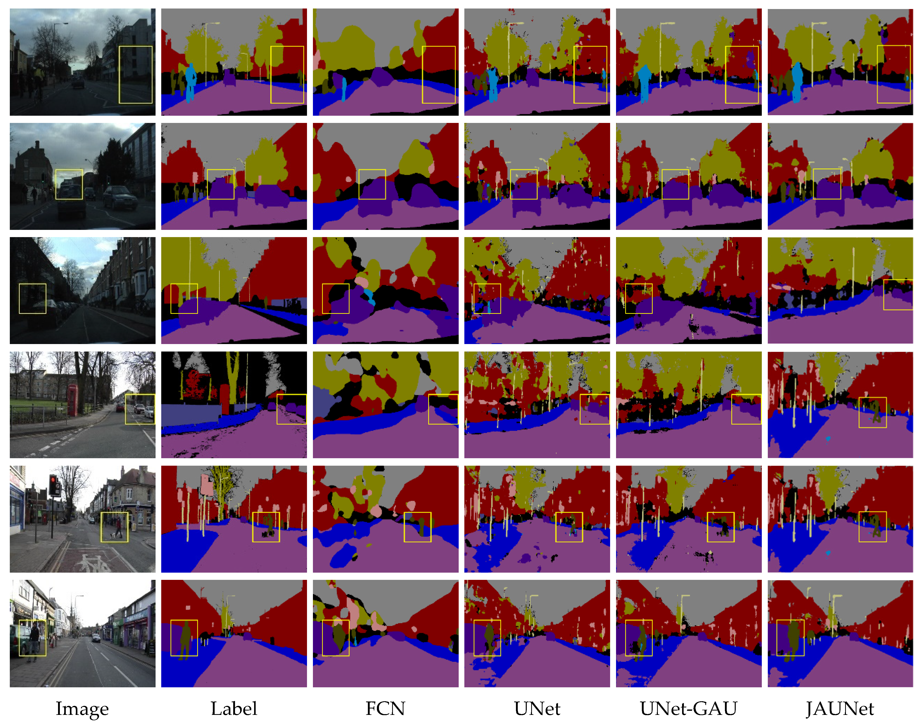
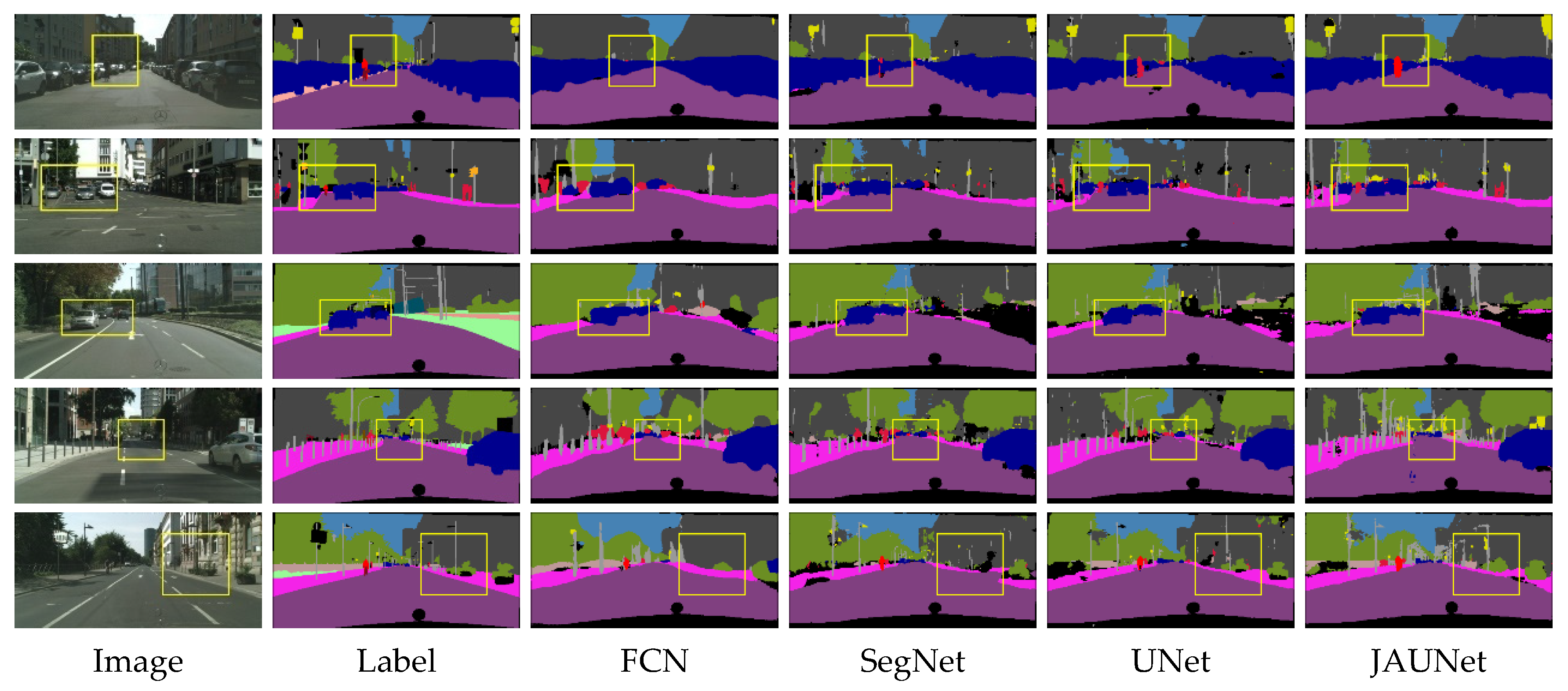
A comparison of the semantic segmentation results of the four networks on the CamVid dataset with the original and labeled images is shown in Figure 10. In the figure, images from left to right are the input images, and labeled images and segmentation results of each network are presented in order.

As shown in Figure 10, where the first group of images has one vehicle target and several pedestrian targets, FCN can recognize pedestrians and vehicles, but the edge segmentation and that of the road are blurred. The UNet-GAU can recognize the pedestrian target on the left side, but mis-segmentation occurs in the building part on the right side. The second image shows multi-vehicle and multi-pedestrian targets, and each network can recognize the vehicle targets, but the pedestrian targets are not well recognized. UNet and UNet-GAU are not effective in the overlapping part of pedestrians and buildings on the left side, while the best segmentation for overlapping targets is JAUNet network and the worst segmentation is FCN.

The third set of images are some continuous vehicle targets and a small pedestrian target, from which we can see that JAUNet can roughly identify the location of the traveler, while ordinary UNet is not able to accomplish it, with the appearance of a lot of noise. The fourth group of images is a bright scene of a bend and there are several vehicle targets in the distance. It can be seen that the networks can basically segment the bend contours well and the distant vehicle targets can be effectively identified. The edges of the vehicle contours are shown in detail. The fifth group of pictures is an intersection scene. There is an intentional pedestrian target in the intersection and a pet in the hand of the pedestrian obscures the road. It can be seen that JAUNet has the best segmentation effect on pedestrians and roads among the four networks. The last picture is a straight road scene and there is a line of people on the left side obscuring part of the vehicle. Among the four networks, FCN and JAUNet can identify the vehicle and pedestrian targets. FCN can recognize the situation that the traveler obscures the vehicle, but the segmentation of the contour is not good, and some mis-segmentation of the pedestrian’s leg occurs in the segmentation result of JAUNet, and the segmentation results are good for other targets. The other networks are all inferior to JAUNet for overlapping targets, and UNet-GAU appears to mis-segment the pedestrian as a bicycle. Combining the above images, JAUNet has better results in edge segmentation and small targets in the CamVid dataset compared to other semantic segmentation networks.

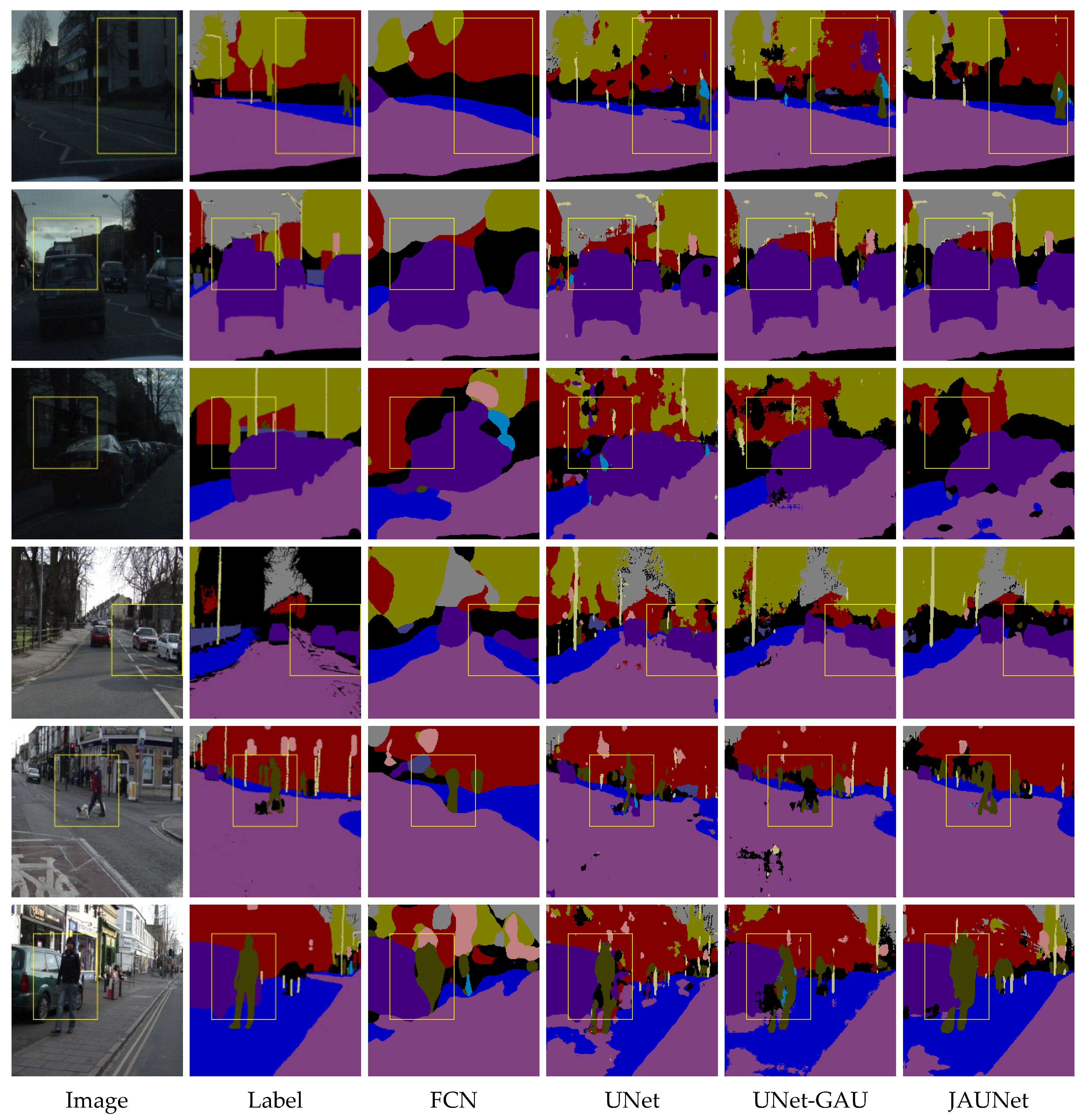
Details of the segmentation results for the CamVid dataset are shown in Figure 11. As can be seen, the differences in the segmentation results of the four networks are outlined in yellow areas in the figure.

After looking closely at the yellow boxed part of the picture, we can see that the first set of images shows the noise that appears in the building and plant parts of UNet, SegNet, and JAUNet, and JAUNet performs the best. All three U-shape network structures can identify the travelers. However, some local missegmentation also occurs in all of them. JAUNet’s mis-segmentation part is smaller, and the edges are more complete, while FCN fails to identify the traveler target at all and is not effective. The second group of images focuses on the segmentation details of the top of the vehicle. All three networks except FCN can segment the vehicle outline well while JAUNet has some small noise. The third group of images focuses on the segmentation details of the continuous vehicles on the left side. Both UNet and UNet-GAU have mis-segmentation of the background part. However, JAUNet has better noise suppression and edge processing in this group of images. For the pedestrian target at the intersection in the fifth group of images, FCN identifies the pedestrian, but the edge segmentation is poor. UNet and UNet-GAU hardly identify the pedestrian, and mis-segmentation occurs. JAUNet can recognize pedestrian targets in the middle of the road and does not divide the pets of pedestrians into roads by mistake. The last set of images shows the details of the pedestrian obscuring the vehicle target. The FCN mis-segments the legs of pedestrians as vehicles, while the UNet and UNet-GAU mis-segment a portion of pedestrians as background. The JAUNet network can recognize the traveler and the vehicle. Although the part of the leg is mis-segmented into the vehicle, it is better than the other networks.

To sum up, during the classification segmentation of CamVid dataset 11, FCN could not segment the object edges well, both UNet and SegNet show much noise in the background, and JAUNet segmentation results are relatively cleaner and had clear edges. In terms of visual effect, the JAUNet network outperforms other networks.

3.5.3. Cityscape Dataset Results

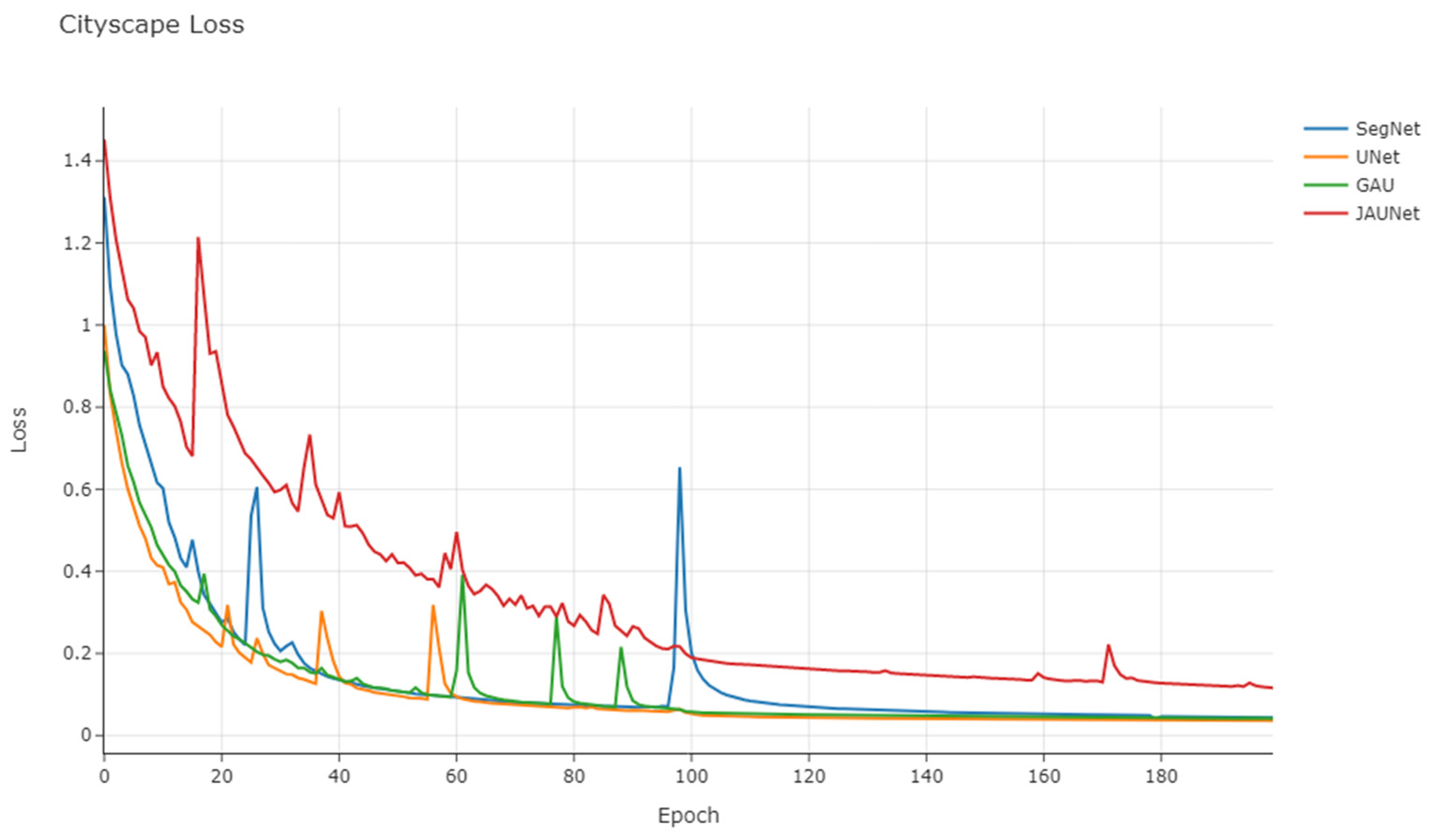
The variation of loss function for the training process of Cityscape dataset is shown in Figure 12.

In the Cityscape dataset, the loss function of JAUNet is slightly higher than the other networks, which may be due to the higher complexity of the network making the convergence slower after the learning rate decreases. Similar to the training of the CamVid dataset, there were some fluctuations in the loss function during the training process, but they all basically leveled off after 100 epochs in the end.

The objective evaluation metrics of the four models on the Cityscape dataset are shown in

Table 6. Evaluation metrics for each model on the Cityscape dataset.

Network	Pretrain	Speed/fps	Params/M	MIoU	FWIoU	GFLOPs
FCN-ResNet34	No	157.10	21.34	49.1	62.1	55.89
ENet	No	41.70	0.36	58.3	65.3	4.35
SegNet	No	35.13	29.45	56.1	65.1	104.54
FastSCNN	No	198.41	1.10	62.8	67.8	1.76
ContextNet [38]	No	176.60	0.88	65.5	71.2	1.78
PSPNet-ResNet18	No	18.73	46.64	63.4	69.6	123.69
GAU	No	35.23	7.94	66.5	73.2	81.64
CGNet [39]	No	44.70	0.50	65.6	71.1	7.00
EDANet	No	105.50	0.68	67.3	73.2	9.00
ICNet	No	30.3	26.5	69.0	76.3	28.3
DFANet A’	No	100	7.8	70.3	77.1	3.4
DFANet B	No	120	4.8	67.1	71.9	2.1
BiSeNetV1_X	ImageNet	105.80	5.80	68.4	75.8	14.90
BiSeNetV1_R	ImageNet	65.50	49.00	74.7	81.3	55.3
UNet	No	36.73	7.76	64.3	70.5	119.03
ConvLSTM_UNet	No	19.23	26.58	64.9	70.1	137.53
JAUNet	No	28.51	33.91	69.1	76.3	137.76

.

The JAUNet proposed in this paper achieves 69.1% mIoU with 33.91 M parameters on the Cityscapes test set. Owing to more training images and higher resolution input images, better segmentation results could be achieved than on the CamVid dataset but accompanied by a decrease in inference speed. Compared to other neural networks, JAUNet can obtain better segmentation accuracy. Like the test results on the CamVid dataset, JAUNet’s segmentation accuracy is higher than that of lightweight networks such as ENet and ContextNet, although the inference speed is slower. Compared with other encoder–decoder network structures, some inference speed is lost, but higher segmentation accuracy is obtained. The segmentation performance of JAUNet is still better than that of GAU, which also adds an attention mechanism, which means that the JAM module is better at extracting channel attention. The segmentation accuracy of JAUNet is similar to that of the Xception39-based network but inferior to that of the ResNet18-based network when compared to the BiSeNetV1 network pre-trained on ImageNet, which is already very good without pre-training on a large dataset. We also give results on the Cityscape dataset using ConvLSTM and UNet alone. Similar to CamVid, using the ConvLSTM module alone does not show much improvement for UNet, and we speculate that the slow convergence may be caused by too many parameters. The simultaneous use of the ConvLSTM and JAM modules also has a better performance on the Cityscape dataset.

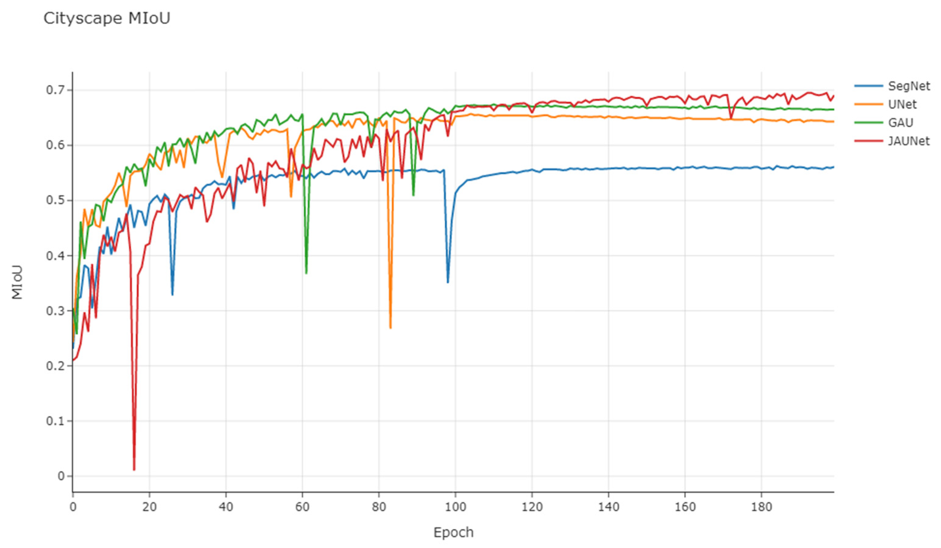
Figure 13 shows the variation of the validation set mIoU with the number of training rounds on the Cityscape dataset. On this dataset, SegNet’s mIoU differs more from other UNet-based networks due to its use of only pooled index-assisted upsampling. JAUNet, on the other hand, has a higher segmentation accuracy than the UNet network after training 110 epochs, although its upsampling speed is slower. This is the same as the results obtained from testing on the CamVid dataset, which further illustrates the effectiveness of the JAM attention module.

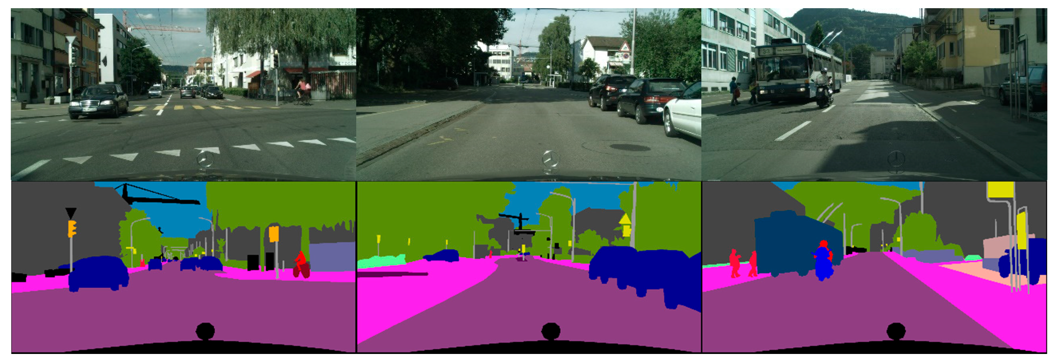
The second set of images is an intersection scene, where there are some side-by-side vehicles in opposite directions, and the segmentation effect of each network on vehicle targets is good. Compared with other networks, JAUNet has a complete segmentation effect on rod-shaped objects and an advantageous effect on small targets such as pedestrians. The third and fourth groups of images are road scenes and several opposite vehicle targets, and we can pay attention to the processing of vehicle edges and rod-shaped objects. JAUNet has the best results.

In the Figure 14, it can also be seen that JAUNet has mis-segmented some of the road markings as car targets, probably because JAUNet is more sensitive to small targets and the markings are not labelled. At the same time, JAUNet classifies the signage target shown as background in the label on the right as a wayfinding sign as well, while the rest of the network would classify the target as a building. This shows that JAUNet classification results seem to be closer to human perception in the classification of targets without labels. The fifth group of images is mainly roads. The segmentation of road edges by FCN is completely blurred. SegNet can recognize part of the edges but mistakenly segmented part of the sidewalks as roads. UNet and JAUNet can segment road edges better, but UNet has poor recognition of the right-side streetlights, and JAUNet with added attention mechanism can be well recognized.

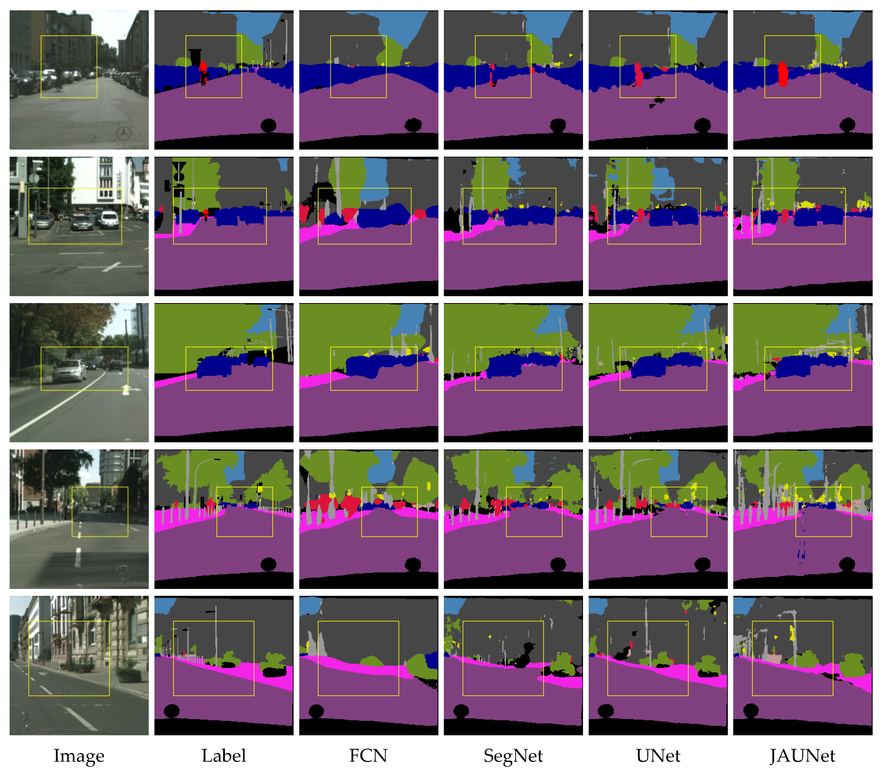
The segmentation details of the Cityscapes dataset are shown in Figure 15. The yellow boxes in the figure mark the parts of the segmentation results that are significantly different. In the detailed diagram, it is obvious to see the mis-segmentation of vehicles on the right side of the first set of images, and JAUNet has the best overall performance. At the same time, other networks classified part of the person target on the left into a car, while UNet can recognize person’s outlines, and JAUNet tends to highlight small target person more. From the second row in the figure, it can be seen that, compared with the network shown, JAUNet can successfully segment the detailed information in the fine objects; in other words, the light pole of the streetlight is successfully recovered, mainly due to the multi-scale fusion of deep and shallow features by the JAM module in the network. Moreover, the results from the first, third, and fourth rows in the figure show that JAUNet is able to perform more accurately, such as the classification of large areas of foliage and ground, as well as the classification of walls and pavements, further demonstrating the enhanced effect of the JAM module for multi-scale information fusion. Compared with other models, JAUNet is able to segment not only objects with fine edges but also larger objects more accurately with significant segmentation effects, indicating that JAUNet has some enhancement in real-time semantic segmentation for different scales of objects.

3.6. Summary of Segmentation Results

Based on the semantic segmentation results and objective evaluation metrics in the previous section, we can find that the basic FCN network performs similarly in both datasets with good objective evaluation metrics, but the actual visual segmentation is poor. FCN can only recognize the target but cannot distinguish the outline. SegNet, on the other hand, can recognize the edges of objects to a certain extent, but there are often cases of mis-segmentation and burrs on the segmented edges. The edge segmentation of UNet is smoother, but mis-segmentation occurs in the background part. Finally, the JAUNet network structure designed in this paper shows that there are differences in the performance of the network in the two datasets. The performance in the CamVid dataset is better, as the object edges can be extracted well, there are few mis-segmentations in the background part, and the objective evaluation index of the test set is also the highest. However, its substantial number of parameters and slower inference speed remain weaknesses in autonomous driving scenarios, which will be the direction of our future research. It can also be found in the segmentation results of each group that JAUNet is more sensitive to the recognition of small targets, which is in line with our expectations for JAM. It should be noted that the final upsampling of JAM compresses the number of channels to the number of categories (19 for Cityscapes and 11 for CamVid), resulting in a slight difference in the number of parameters between the Cityscapes and CamVid datasets.

4. Conclusions

Segmentation technology of traffic road images, as an important part of autonomous driving technology, plays a significant role in new energy vehicles and new travel modes and has received extensive attention from major car companies in various countries with good prospects. Although the traditional image segmentation technology can extract the target to a certain extent, it cannot meet the requirements of autonomous driving scenarios due to the need for manual feature extraction, poor generalization ability of the model, and the inability of the clustering algorithm to label the pixel points with semantic information. In addition, with the rapid development of computer hardware and software level, artificial intelligence technology has been updated rapidly in recent years, and deep learning semantic segmentation technology has become the mainstream of image segmentation technology. In this paper, starting from the actual application scenario, combining the characteristics of continuous images obtained in the automatic interpretation process and targeting at the mining of contextual information in continuous images, the basic technical principles of deep learning semantic segmentation, JAM attention mechanism, and ConvLSTM network structure are integrated to systematically study and design the JAUNet semantic segmentation network model. Compared with other existing methods, the proposed method in this paper performs more outstandingly on mIoU evaluation. Compared with the common UNet, this paper improves its jump connection part to make up for the lack of processing of low-dimensional features, so that the upsampling process can better figure-restore the image features and the model ground mIoU evaluation index can reach 63.7% and 73.2%, respectively. The experimental results on the CamVid dataset and the Cityscapes dataset show that this model has high average detection accuracy.

References

1. Mehrotra, R.; Namuduri, K.R.; Ranganathan, N. Gabor filter-based edge detection. Pattern Recognit. 1992, 25, 1479–1494. [Google Scholar] [CrossRef]
2. Krizhevsky, A.; Sutskever, I.; Hinton, G.E. Imagenet classification with deep convolutional neural networks. Adv. Neural Inf. Process. Syst. 2012, 25, 84–90. [Google Scholar] [CrossRef] [Green Version]
3. He, K.; Zhang, X.; Ren, S.; Sun, J. Deep residual learning for image recognition. In Proceedings of the IEEE Conference on Computer Vision and Pattern Recognition, Las Vegas, NV, USA, 27–30 June 2016; pp. 770–778. [Google Scholar]
4. Chen, L.-C.; Papandreou, G.; Kokkinos, I.; Murphy, K.; Yuille, A.L. Semantic image segmentation with deep convolutional nets and fully connected crfs. arXiv 2014, arXiv:1412.7062. [Google Scholar]
5. Noh, H.; Hong, S.; Han, B. Learning deconvolution network for semantic segmentation. In Proceedings of the IEEE International Conference on Computer Vision, Santiago, Chile, 7–13 December 2015; pp. 1520–1528. [Google Scholar]
6. Zeiler, M.D.; Krishnan, D.; Taylor, G.W.; Fergus, R. Deconvolutional networks. In Proceedings of the 2010 IEEE Computer Society Conference on Computer Vision and Pattern Recognition, San Francisco, CA, USA, 13–18 June 2010; pp. 2528–2535. [Google Scholar]
7. Mikolov, T.; Kombrink, S.; Burget, L.; Černocký, J.; Khudanpur, S. Extensions of recurrent neural network language model. In Proceedings of the 2011 IEEE International Conference on Acoustics, Speech and Signal Processing (ICASSP), Prague, Czech Republic, 22–27 May 2011; pp. 5528–5531. [Google Scholar]
8. Wang, Z.; Xia, M.; Lu, M.; Pan, L.; Liu, J. Parameter Identification in Power Transmission Systems Based on Graph Convolution Network. IEEE Trans. Power Deliv. 2021, 37, 3155–3163. [Google Scholar] [CrossRef]
9. Chen, L.-C.; Papandreou, G.; Schroff, F.; Adam, H. Rethinking atrous convolution for semantic image segmentation. arXiv 2017, arXiv:1706.05587. [Google Scholar]
10. Zhao, H.; Shi, J.; Qi, X.; Wang, X.; Jia, J. Pyramid scene parsing network. In Proceedings of the IEEE Conference on Computer Vision and Pattern Recognition, Honolulu, HI, USA, 21–26 July 2017; pp. 2881–2890. [Google Scholar]
11. Gao, J.; Weng, L.; Xia, M.; Lin, H. MLNet: Multichannel feature fusion lozenge network for land segmentation. J. Appl. Remote Sens. 2022, 16, 016513. [Google Scholar] [CrossRef]
12. Chen, B.; Xia, M.; Qian, M.; Huang, J. MANet: A multi-level aggregation network for semantic segmentation of high-resolution remote sensing images. Int. J. Remote Sens. 2022, 43, 5874–5894. [Google Scholar] [CrossRef]
13. Song, L.; Xia, M.; Weng, L.; Lin, H.; Qian, M.; Chen, B. Axial Cross Attention Meets CNN: Bi-Branch Fusion Network for Change Detection. IEEE J. Sel. Top. Appl. Earth Obs. Remote Sens. 2022, 16, 32–43. [Google Scholar] [CrossRef]
14. Ronneberger, O.; Fischer, P.; Brox, T. U-net: Convolutional networks for biomedical image segmentation. In Proceedings of the International Conference on Medical Image Computing and Computer-Assisted Intervention, Munich, Germany, 5–9 October 2015; pp. 234–241. [Google Scholar]
15. Badrinarayanan, V.; Kendall, A.; Cipolla, R. Segnet: A deep convolutional encoder-decoder architecture for image segmentation. IEEE Trans. Pattern Anal. Mach. Intell. 2017, 39, 2481–2495. [Google Scholar] [CrossRef]
16. Peng, C.; Zhang, X.; Yu, G.; Luo, G.; Sun, J. Large kernel matters—Improve semantic segmentation by global convolutional network. In Proceedings of the IEEE Conference on Computer Vision and Pattern Recognition, Honolulu, HI, USA, 21–26 July 2017; pp. 4353–4361. [Google Scholar]
17. Bilinski, P.; Prisacariu, V. Dense decoder shortcut connections for single-pass semantic segmentation. In Proceedings of the IEEE Conference on Computer Vision and Pattern Recognition, Salt Lake City, UT, USA, 18–23 June 2018; pp. 6596–6605. [Google Scholar]
18. Hu, J.; Shen, L.; Sun, G. Squeeze-and-excitation networks. In Proceedings of the IEEE Conference on Computer Vision and Pattern Recognition, Salt Lake City, UT, USA, 18–23 June 2018; pp. 7132–7141. [Google Scholar]
19. Woo, S.; Park, J.; Lee, J.-Y.; Kweon, I.S. Cbam: Convolutional block attention module. In Proceedings of the European Conference on Computer Vision (ECCV), Munich, Germany, 8–14 September 2018; pp. 3–19. [Google Scholar]
20. Li, H.; Xiong, P.; An, J.; Wang, L. Pyramid attention network for semantic segmentation. arXiv 2018, arXiv:1805.10180. [Google Scholar]
21. Shi, X.; Chen, Z.; Wang, H.; Yeung, D.-Y.; Wong, W.-K.; Woo, W.-C. Convolutional LSTM network: A machine learning approach for precipitation nowcasting. In Proceedings of the Twenty-ninth Conference on Neural Information Processing Systems, Montréal, QC, Canada, 7–12 December 2015; Volume 28. [Google Scholar]
22. Simonyan, K.; Zisserman, A. Very deep convolutional networks for large-scale image recognition. arXiv 2014, arXiv:1409.1556. [Google Scholar]
23. Liu, W.; Rabinovich, A.; Berg, A.C. Parsenet: Looking wider to see better. arXiv 2015, arXiv:1506.04579. [Google Scholar]
24. Hong, S.; Noh, H.; Han, B. Decoupled deep neural network for semi-supervised semantic segmentation. In Proceedings of the Twenty-ninth Conference on Neural Information Processing Systems, Montréal, QC, Canada, 7–12 December 2015; Volume 28. [Google Scholar]
25. Lu, C.; Xia, M.; Lin, H. Multi-scale strip pooling feature aggregation network for cloud and cloud shadow segmentation. Neural Comput. Appl. 2022, 34, 6149–6162. [Google Scholar] [CrossRef]
26. Miao, S.; Xia, M.; Qian, M.; Zhang, Y.; Liu, J.; Lin, H. Cloud/shadow segmentation based on multi-level feature enhanced network for remote sensing imagery. Int. J. Remote Sens. 2022, 43, 5940–5960. [Google Scholar] [CrossRef]
27. Qu, Y.; Xia, M.; Zhang, Y. Strip pooling channel spatial attention network for the segmentation of cloud and cloud shadow. Comput. Geosci. 2021, 157, 104940. [Google Scholar] [CrossRef]
28. Brostow, G.J.; Fauqueur, J.; Cipolla, R. Semantic object classes in video: A high-definition ground truth database. Pattern Recognit. Lett. 2009, 30, 88–97. [Google Scholar] [CrossRef]
29. Cordts, M.; Omran, M.; Ramos, S.; Rehfeld, T.; Enzweiler, M.; Benenson, R.; Franke, U.; Roth, S.; Schiele, B. The cityscapes dataset for semantic urban scene understanding. In Proceedings of the IEEE Conference on Computer Vision and Pattern Recognition, Las Vegas, NV, USA, 27–30 June 2016; pp. 3213–3223. [Google Scholar]
30. Keskar, N.S.; Socher, R. Improving generalization performance by switching from adam to sgd. arXiv 2017, arXiv:1712.07628. [Google Scholar]
31. Sturgess, P.; Alahari, K.; Ladicky, L.; Torr, P.H. Combining appearance and structure from motion features for road scene understanding. In Proceedings of the BMVC-British Machine Vision Conference, London, UK, 7–10 September 2009. [Google Scholar]
32. Tighe, J.; Lazebnik, S. Superparsing: Scalable nonparametric image parsing with superpixels. In Proceedings of the European Conference on Computer Vision, Heraklion, Greece, 5–11 September 2010; pp. 352–365. [Google Scholar]
33. Paszke, A.; Chaurasia, A.; Kim, S.; Culurciello, E. Enet: A deep neural network architecture for real-time semantic segmentation. arXiv 2016, arXiv:1606.02147. [Google Scholar]
34. Watanabe, S.; Hori, T.; Karita, S.; Hayashi, T.; Nishitoba, J.; Unno, Y.; Soplin, N.E.Y.; Heymann, J.; Wiesner, M.; Chen, N. Espnet: End-to-end speech processing toolkit. arXiv 2018, arXiv:1804.00015. [Google Scholar]
35. Zhao, H.; Qi, X.; Shen, X.; Shi, J.; Jia, J. Icnet for real-time semantic segmentation on high-resolution images. In Proceedings of the European Conference on Computer Vision (ECCV), Munich, Germany, 8–14 September 2018; pp. 405–420. [Google Scholar]
36. Li, H.; Xiong, P.; Fan, H.; Sun, J. Dfanet: Deep feature aggregation for real-time semantic segmentation. In Proceedings of the IEEE/CVF Conference on Computer Vision and Pattern Recognition, Long Beach, CA, USA, 15–20 June 2019; pp. 9522–9531. [Google Scholar]
37. Yu, C.; Wang, J.; Peng, C.; Gao, C.; Yu, G.; Sang, N. Bisenet: Bilateral segmentation network for real-time semantic segmentation. In Proceedings of the European Conference on Computer Vision (ECCV), Munich, Germany, 8–14 September 2018; pp. 325–341. [Google Scholar]
38. Han, W.; Zhang, Z.; Zhang, Y.; Yu, J.; Chiu, C.-C.; Qin, J.; Gulati, A.; Pang, R.; Wu, Y. Contextnet: Improving convolutional neural networks for automatic speech recognition with global context. arXiv 2020, arXiv:2005.03191. [Google Scholar]
39. Wu, T.; Tang, S.; Zhang, R.; Cao, J.; Zhang, Y. Cgnet: A light-weight context guided network for semantic segmentation. IEEE Trans. Image Process. 2020, 30, 1169–1179. [Google Scholar] [CrossRef] [PubMed]
Figure 1. Network structure of the method in this paper.
Applsci 13 01493 g001
Figure 2. UNet network structure adapted with permission from Ref. [14]. Copyright 2015, copyright Ronneberger.
Applsci 13 01493 g002
Figure 3. ConvLSTM.
Applsci 13 01493 g003
Figure 4. Jump attention module.
Applsci 13 01493 g004
Figure 5. Channel attention.
Applsci 13 01493 g005
Figure 6. Sample of the CamVid dataset.
Applsci 13 01493 g006
Figure 7. Sample of the Cityscapes dataset.
Applsci 13 01493 g007
Figure 8. CamVid train loss.
Applsci 13 01493 g008
Figure 9. CamVid MIoU.
Applsci 13 01493 g009
Figure 10. Segmentation results of each network on the CamVid dataset.
Applsci 13 01493 g010
Figure 11. Details of segmentation results for each network on the CamVid dataset.
Applsci 13 01493 g011
Figure 12. Cityscape train loss.
Applsci 13 01493 g012
Figure 13. Cityscape MIoU.
Applsci 13 01493 g013
Figure 14. Segmentation results of each network on the Cityscapes dataset.
Applsci 13 01493 g014
Figure 15. Details of the segmentation results for each network on the Cityscape dataset.
Applsci 13 01493 g015