Improving Semi-Supervised Image Classification by Assigning Different Weights to Correctly and Incorrectly Classified Samples

Abstract

Semi-supervised deep learning, a model that aims to effectively use unlabeled data to help learn sample features from labeled data, is a recent hot topic. To effectively use unlabeled data, a new semi-supervised learning model based on a consistency strategy is proposed. In the supervised part with labeled samples, the image generation model first generates some artificial images to complement the limited number of labeled samples. Secondly, the sample label mapping, as the “benchmark”, is compared to the corresponding sample features in the network as an additional loss to complement the original supervisory loss, aiming to better correct the model parameters. Finally, the original supervised loss is changed so that the network parameters are determined by the characteristics of each correctly classified sample. In the unsupervised part, the actual unsupervised loss is altered so that the model does not “treat all samples equally” and can focus more on the characteristics of misclassified samples. A total of 40 labeled samples from the CIFAR-10 and SVHN datasets were used to train the semi-supervised model achieving accuracies of 93.25% and 96.83%, respectively, demonstrating the effectiveness of the proposed semi-supervised model.

1. Introduction

Early image classification research [1,2] relied on the manual collection of image features, such as color and texture, to classify images accurately. However, this early work was time-consuming and laborious and may cause the misclassification of images due to the large number of pictures and people’s inattentiveness. In recent years, with the rise of neural networks [3,4,5,6,7] and large datasets, tremendous progress has been made in many tasks in computer vision, such as image classification [8,9], image segmentation [10,11], and object detection [12,13,14].

This paper focuses on semi-supervised image classification methods, which learn sample features from a small portion of labeled data and a large amount of unlabeled data to classify images accurately. This ensures less human workload and higher accuracy of image classification. Based on an extensive review [15,16,17,18], it can be found that the existing semi-supervised learning methods can be broadly classified into three categories. (1) Adversarial learning-based methods [19,20,21,22], (2) Graph-based methods [23,24], and (3) Consistency strategy-based methods [25,26,27,28,29,30,31,32,33].

The adversarial learning-based methods [19,20,21,22] generate many artificial images to complement the actual training samples by learning the underlying distribution of real images. The aim is to obtain CNN models with better performance by increasing the training data. In recent years, generative adversarial networks and their variants [34,35,36,37] have been extensively studied and applied to semi-supervised and unsupervised learning with good results.

Methods based on consistency strategies [30,31,32,33] effectively use information from unlabeled data by making the two predicted values of different images produced by random enhancement consistent. For example, pseudo-label [25] uses the network output directly as the consistency target. Temporal ensembling [26] uses the exponential moving average (EMA) predictions from each unlabeled data as the consistency target, mainly improving the quality of the target. The mean teacher [27] framework does not retain the exponential moving average (EMA) predictions. Instead, it uses the exponential average weights from the student model to reconstruct the teacher model, which ensures target quality and eliminates the redundant matrix information associated with exponential average shifts. VAT [28] enables the model to generate more reliable consistency targets by enhancing local smoothing of the label distribution for a given input. Liu et al. [29] judged sample predictions and rejected and excluded unreliable samples. Focal loss [38] and reduced focal loss [39] focus more on hard-to-classify examples by simply weighting the losses. Liu et al. [40,41] have unexpected effects by exploring sample information within the network.

In this paper, a new semi-supervised classification model is proposed. Specifically, in the supervised part, the image generation model generates several artificial samples with labels (with “almost the same” underlying distribution as the actual training samples), aiming to complement the limited number of labeled samples; secondly, the sample labels are mapped to the interior of the network as a “benchmark” to compare with the internal features of the samples as part of the supervised loss. Finally, the original supervisory loss is weighted to enable the network to correct misclassified samples accurately. In the unsupervised part, unlike the actual unsupervised loss, we filter the samples individually so that the network parameters are dominated by the features of the examples judged to be correct. The above process allows the semi-supervised model to learn sample features more accurately, thus enabling the model to classify images accurately.

The main contributions are as follows:

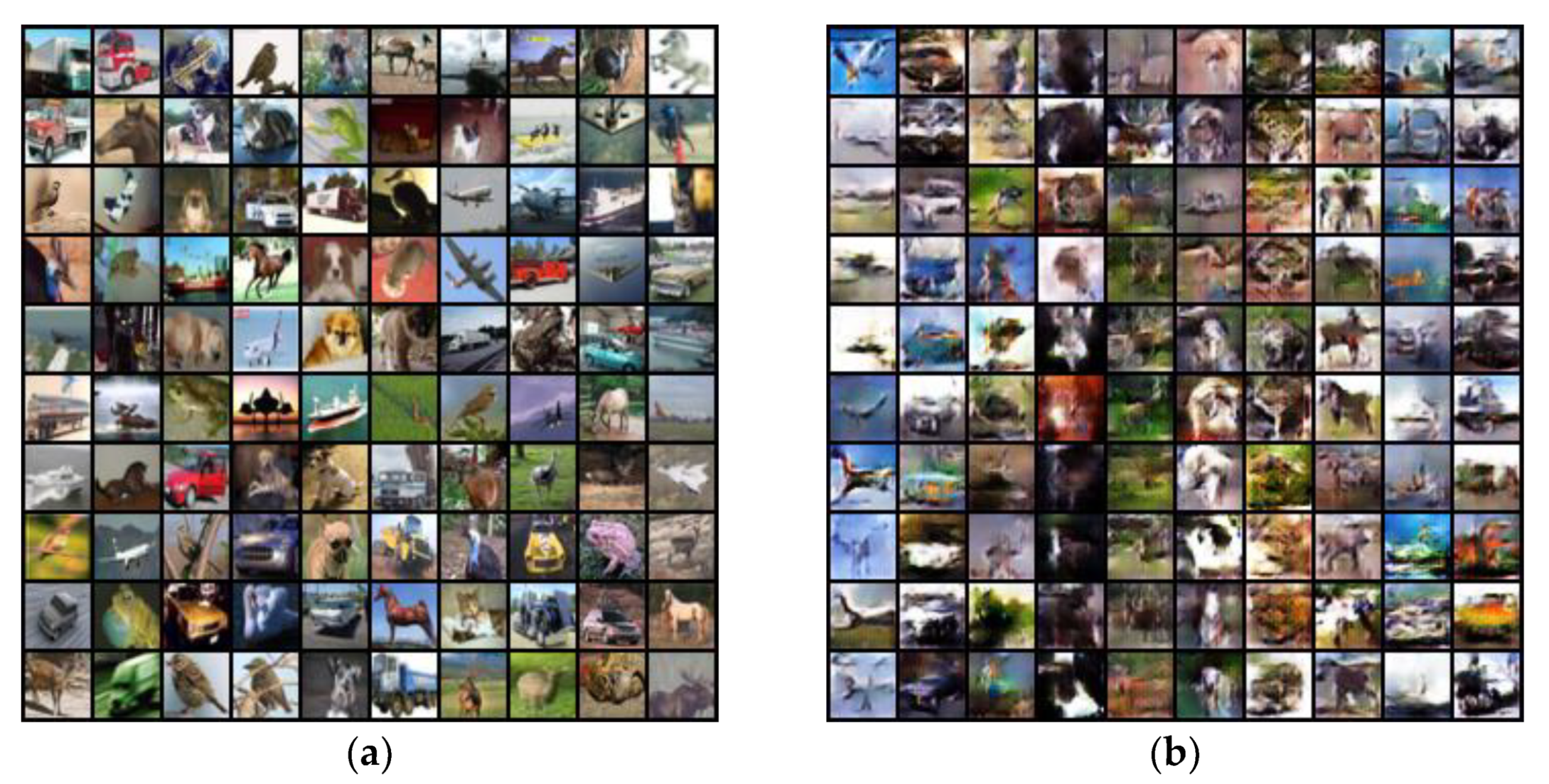
• A new image generation model is proposed to generate artificial samples designed to complement the limited number of labeled samples in the supervised modules.
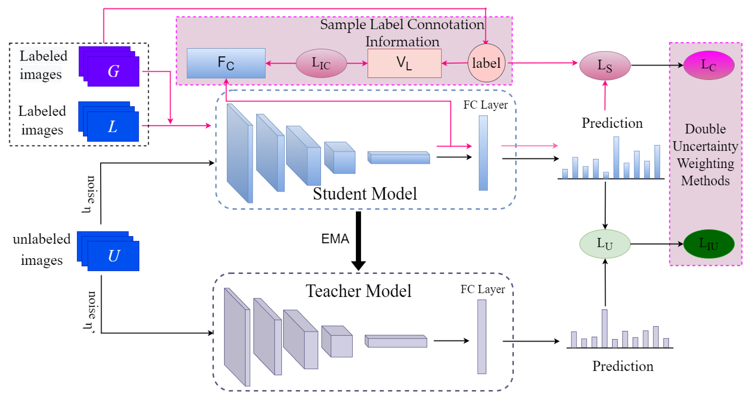
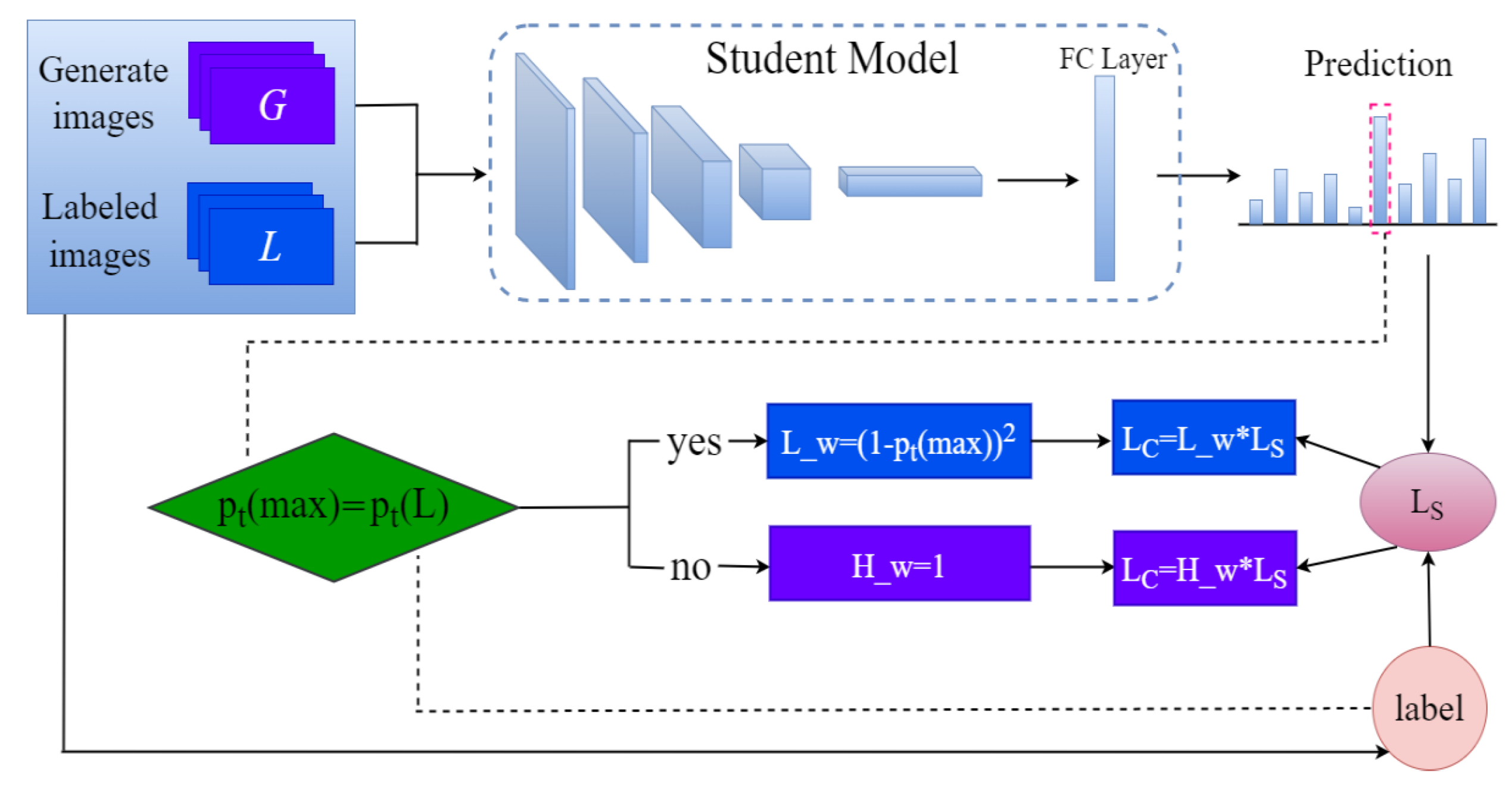
• In the supervisory loss section, the sample labels are compared with the sample predictions one by one, weighting the original loss and introducing additional losses to supplement the supervisory loss.
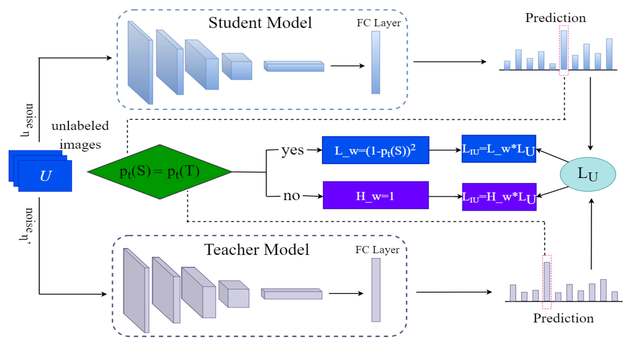
• In the unsupervised loss section, judgment conditions are added so that the correctly classified sample features dominate the network parameters.

2. Related Work

In this section, a series of introductory modules used in previous semi-supervised learning are reviewed, and then initial ideas for improving them are presented, given their shortcomings.

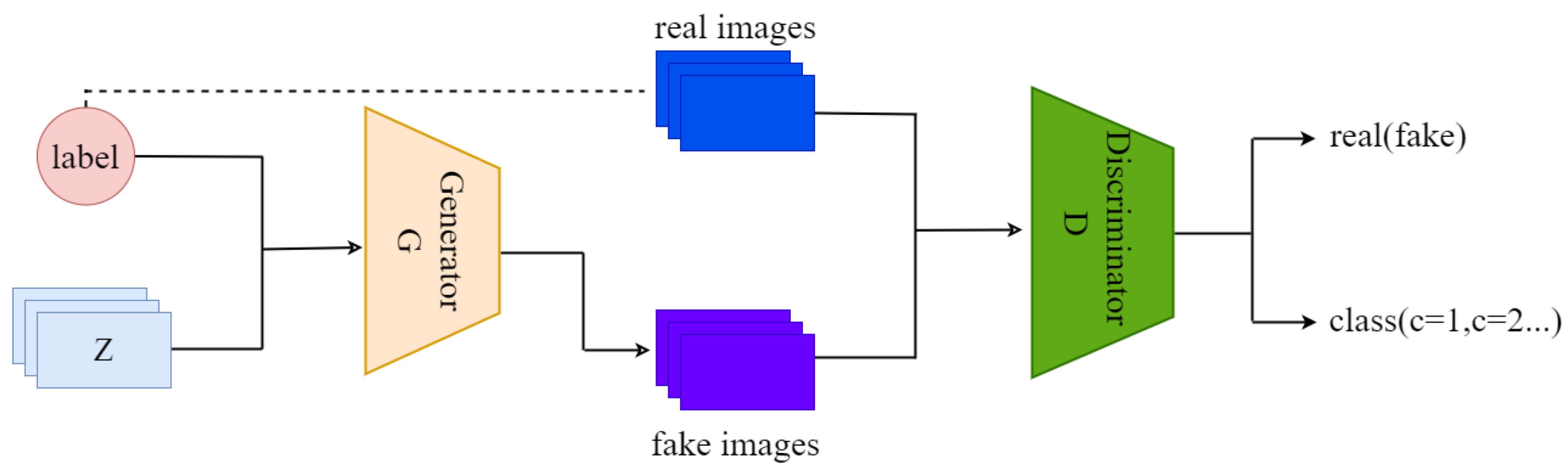
2.1. Conditional Image Synthesis with Auxiliary Classifier GANS

The existing semi-supervised classification models based on adversarial learning use generative adversarial networks (GANS) [34] to generate some artificial images without labels to assist in image classification. In contrast, ACGAN [37] can directly generate the random noise Z into an artificial image with labels, which is the difference between them. As shown in Figure 1, ACGAN [37] consists of two models: the generator and the discriminator. First, a random noise Z and a randomly given label are fed into the generator to generate a fake image, which may be blurred or perhaps even just a random combination of pixel points. Then, the generated fake images are fed into the discriminator along with the real samples, and the discriminator needs to recognize the authenticity of these images and classify them accurately.

$${\mathrm{L}}_{\mathrm{S}}=\mathrm{E}[\mathrm{logP}\left({\mathrm{S}=\mathrm{real}|\mathrm{X}}_{\mathrm{real}}\right)+\mathrm{logP}\left({\mathrm{S}=\mathrm{fake}|\mathrm{X}}_{\mathrm{fake}}\right)]$$

(1)

$${\mathrm{L}}_{\mathrm{C}}=\mathrm{E}[\mathrm{logP}\left({\mathrm{C}=\mathrm{c}|\mathrm{X}}_{\mathrm{real}}\right)+\mathrm{logP}\left({\mathrm{C}=\mathrm{c}|\mathrm{X}}_{\mathrm{fake}}\right)]$$

(2)

Here, ${\mathrm{L}}_{\mathrm{S}}$ represents the discriminator’s ability to identify “true” as “true” and “false” as “false”, and ${\mathrm{L}}_{\mathrm{C}}$ represents the discriminator’s ability to classify the true and false data correctly. The generator is trained to maximize ${\mathrm{L}}_{\mathrm{C}}$− ${\mathrm{L}}_{\mathrm{S}}$ (the part of ${\mathrm{L}}_{\mathrm{S}}$ and ${\mathrm{L}}_{\mathrm{C}}$ about which the actual image is independent of the generator), which means that the data generated by the generator is more realistic and has the highest probability of being correctly classified. The discriminator is trained to maximize ${\mathrm{L}}_{\mathrm{C}}$+${ \mathrm{L}}_{\mathrm{S}}$, that is, to maximize the discriminator’s ability to organize and discriminate between real and fake data.

The authors of [42,43] argue that if a discriminator is given two incompatible tasks (recognizing image authenticity and classification), then the discriminator’s performance in both areas will degrade. We have added a third classification model to ACGAN (this is where we differ). As shown in Figure 2, in the model for generating artificial images, the discriminator has only the unique task of recognizing image authenticity.

2.2. Semi-Supervised Image Classification Models

The semi-supervised image classification model based on the consistent regularization strategy is given as dataset ${\mathrm{D} = \mathrm{D}}_{\mathrm{L}}\cup {\mathrm{D}}_{\mathrm{U}}$, where the data in ${\mathrm{D}}_{\mathrm{L}}$ is manually labeled while the data in ${\mathrm{D}}_{\mathrm{U}}$ is unlabeled [34]. It aims to use dataset $\mathrm{D}$ to train a CNN model that can accurately classify images of different categories (contained in ${\mathrm{D}}_{\mathrm{L}}$) in the test data. Existing semi-supervised image classification models are divided into two parts: the fully supervised modules with labeled data ${\mathrm{D}}_{\mathrm{L}}$ and the unsupervised modules with unlabeled data ${\mathrm{D}}_{\mathrm{U}}$.

2.2.1. Full Supervised Modules

As shown in Figure 3, the semi-supervised classification model adjusts the model parameters by feeding the data inside D into the student model, obtaining their predicted values, and then comparing them with the actual labels of these data. Its loss function is defined as Equation (3).

$${\mathrm{L}}_{\mathrm{S}}=-\left(\mathrm{ylog}\mathrm{y}\prime +\left(1-\mathrm{y}\right)\log \left(1-\mathrm{y}\prime \right)\right)$$

(3)

Here, $\mathrm{y}$ and $\mathrm{y}\prime$ represent the actual labels of the samples and their predicted values, respectively. The excellent performance of the student model is inextricably linked to the amount of data, so the image generation model is used to generate some artificial images designed to complement the real sample.

The authors believe that the training samples in the dataset should be given different weight shares based on the accuracy of their judgment results. The original supervised loss only calculates the difference between the sample labels and the predicted values. The model parameters cannot be dominated by the characteristics of the correctly judged samples (i.e., examples of incorrect judgments remain uncorrected in subsequent training). While Zhou Z. [41] et al. mitigated this problem by setting a threshold for supervised loss that grows with model refinement, it still does not allow the semi-supervised model to locate the wrong samples accurately. Therefore, instead of formulating a threshold, we compare the label of each sample with the predicted value to clarify the correctness of each judged sample and then weigh these sample losses before allowing future training to be “on target.” This means that previously misclassified samples will have a higher probability of being correctly classified in future training.

While Liu et al. [40,41] had good results by examining the semantic information inherent in the samples, they explored unlabeled samples. The authors believe that it is more advantageous to map the labels inside the network as a ‘benchmark’ against the intrinsic features of the samples. This is because, like solving a problem, only when the correct answer is known can learning be derived from it to ensure that it is right next time.

2.2.2. Unsupervised Modules

Based on the assumption of the consistency principle [30,31,32,33], one image with the same underlying distribution still has the same class labels for its predictions after adding different perturbation methods, as in Figure 4, by adding other perturbation methods (η, η′) to the data inside ${\mathrm{D}}_{\mathrm{U}}$. Then, the two predicted labels generated by the two images of the student model and the teacher model are forced to agree to learn the potential features in the unlabeled samples. Its loss function is defined as Equation (4).

$${\mathrm{L}}_{\mathrm{U}}={\displaystyle \sum }_{\mathrm{x}\in \left\{\mathrm{D}\right\}}{\mathrm{E}}_{\mathsf{\eta },\mathsf{\eta }},\parallel \mathrm{f}\left(\mathrm{x},{\mathsf{\theta }}^{\prime },{\mathsf{\eta }}^{\prime }\right)-\mathrm{f}\left(\mathrm{x},\mathsf{\theta },\mathsf{\eta }\right){\parallel }_2^2$$

(4)

Here, $\mathrm{x}$ represents all samples (with and without labels) in the training set and $\mathrm{f}\left({\mathrm{x},\mathsf{\theta }}^{\prime }{,\mathsf{\eta }}^{\prime }\right)$ and $\mathrm{f}\left(\mathrm{x},\mathsf{\theta },\mathsf{\eta }\right)$ are the predicted values obtained for $\mathrm{x}$ under different weights and perturbations for ${(\mathsf{\theta }}^{\prime }{,\mathsf{\eta }}^{\prime })$ and $(\mathsf{\theta },\mathsf{\eta }$), respectively.

The original unsupervised loss compares two predictions of an image under different perturbations, then sums these results and averages them. A conditional judgment is added when comparing these two predicted values. If they are the same, a smaller weight is given, and if they are different, a more prominent weight is given. This ensures that the sample features can be learned more fully during the future training of the model so that the two predicted values of a sample can be more consistent. This is also more in line with our consistency strategy.

3. Proposed Methods

As shown in Figure 5, the semi-supervised model can generate some artificial samples through the image generation model, designed to supplement the limited training data in the supervised part. The supervised loss consists of two components, L_C and ${\mathrm{L}}_{\mathrm{IC}}$. ${\mathrm{L}}_{\mathrm{C}}$ is obtained by weighting the original supervisory loss L_S to make the model focus more on the correctly classified sample features. ${\mathrm{L}}_{\mathrm{IC}}$ represents the additional loss that supplements the supervisory loss ${\mathrm{L}}_{\mathrm{C}}$ by using the sample labels as the “benchmark” to compare with the sample features within the network. The unsupervised loss is ${\mathrm{L}}_{\mathrm{IU}}$.

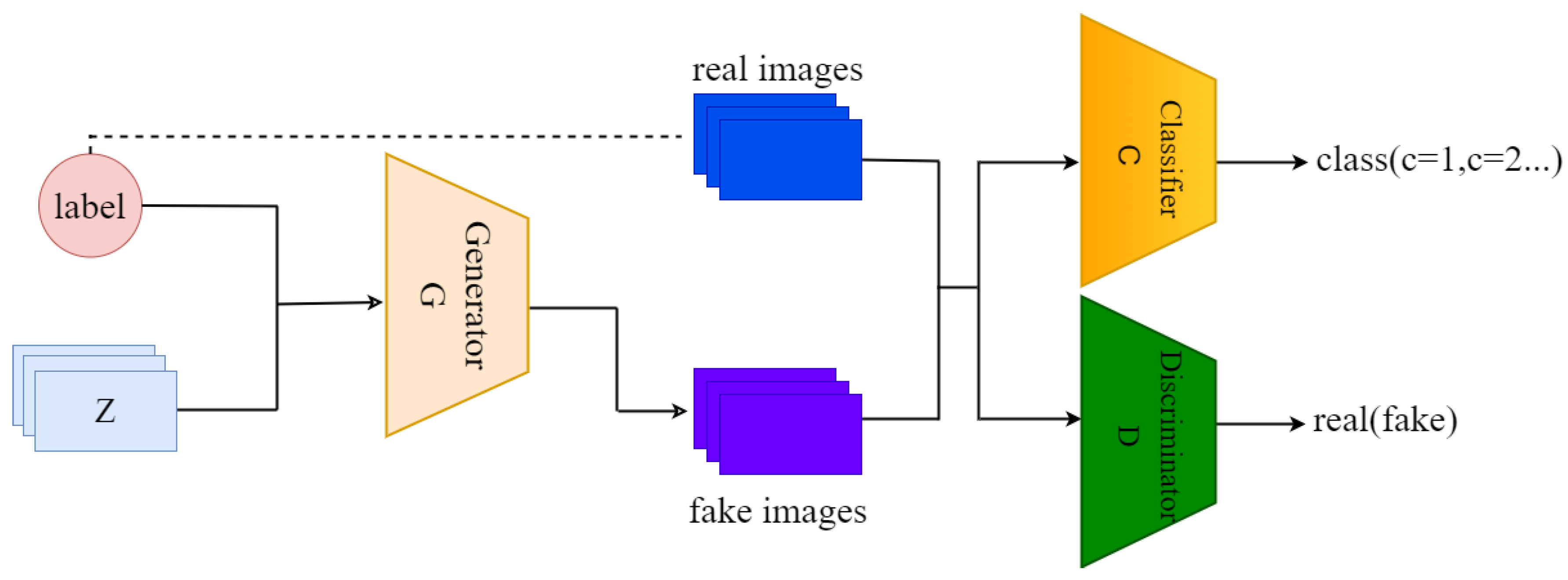
3.1. Image Generation Model

As shown in Figure 2, an image generation model based on ACGAN [37] is introduced. It is believed that artificially generating a portion of images used to supplement the supervised part of the restricted samples can improve the classification performance of the student model. This model consists of three parts: a generator, a discriminator, and a classifier. First, random noise Z and randomly given label information are inputted into the generator to generate fake images. The generated fake images and actual samples are then provided to the discriminator and classifier. The discriminator needs to discriminate the authenticity of these images, and the classifier needs to classify them accurately to improve the model’s discrimination and classification performance. The loss function of the discriminator is defined as Equation (5).

$$\mathrm{L}\left(\mathrm{D}\right)=\mathrm{BCE}\left(\mathrm{D}\left(\mathrm{G}\left(\mathrm{Z}\right)\right),0\right)+\mathrm{BCE}\left(\mathrm{D}\left(\mathrm{x}\right),1\right)+\mathrm{CE}\left(\mathrm{C}\left(\mathrm{G}\left(\mathrm{Z}\right)\right),\mathrm{y}\prime \right)+\mathrm{CE}\left(\mathrm{C}\left(\mathrm{x}\right),\mathrm{y}\right)$$

(5)

The loss function of the classifier is defined as Equation (6).

$$\mathrm{L}\left(\mathrm{C}\right)=\mathrm{CE}\left(\mathrm{C}\left(\mathrm{G}\left(\mathrm{Z}\right)\right),\mathrm{y}\prime \right)+\mathrm{CE}\left(\mathrm{x}, \mathrm{y}\right)$$

(6)

The loss function of the generator is defined as Equation (7).

$$\mathrm{L}\left(\mathrm{G}\right)=\mathrm{BCE}\left(\mathrm{D}\left(\mathrm{G}\left(\mathrm{Z}\right)\right),1\right)+\mathrm{CE}\left(\mathrm{C}\left(\mathrm{G}\left(\mathrm{Z}\right)\right),\mathrm{y}\prime \right)$$

(7)

Here, D, G, and C represent the discriminator, generator, and classifier, respectively, x and y are the actual training sample with its label, Z is the random noise, and y′ is the corresponding label of the generated artificial image. BCE is the binary cross-entropy, and CE is the cross-entropy. To obtain good performance, these generated artificial images are fed into student model training simultaneously with actual samples.

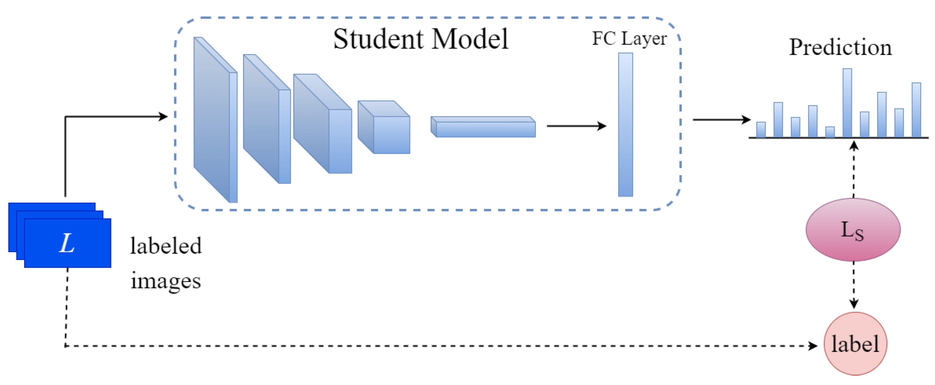
3.2. Supervisory Losses

As shown in Figure 5, our total supervised loss is divided into two parts, ${\mathrm{L}}_{\mathrm{C}}$ and ${\mathrm{L}}_{\mathrm{IC}}$. We feed the artificial images generated on the fly into the student model for training, along with the actual training samples (note that here the fake images are passed into the student model in real-time, so there is no need to save them). The predicted values obtained are then compared with the actual values, as shown below.

We map the sample labels (actual samples vs. artificial samples) as vectors that serve as “benchmarks” to compare with the intrinsic information of the samples in the network as our loss ${\mathrm{L}}_{\mathrm{IC}}$. Specifically, given a small batch of input samples containing B samples, we define the sample intrinsic information map of the L-layer as ${\mathrm{F}}^{\mathrm{L}}\in {\mathrm{R}}^{\mathrm{B}*\mathrm{C}*\mathrm{H}*\mathrm{W}}$, where H and W are the spatial dimensions of the feature map and C is the number of channels, and the matrix obtained by normalizing the intrinsic information of this small batch of input samples is as Equation (8).

$${\mathrm{F}}_{\mathrm{C}}=\left(\frac{\mathrm{F}{\left(\mathrm{x}\right)}_1^{\mathrm{L}}}{\parallel \mathrm{F}{\left(\mathrm{x}\right)}_1^{\mathrm{L}}\parallel },\cdots ,\frac{\mathrm{F}{\left(\mathrm{x}\right)}_{\mathrm{B}}^{\mathrm{L}}}{\parallel \mathrm{F}{\left(\mathrm{x}\right)}_{\mathrm{B}}^{\mathrm{L}}\parallel }\right)$$

(8)

${\mathrm{F}}_{\mathrm{C}}$ denotes the sample feature information of B samples within the network. Similarly, the label information is mapped to a vector with the same number of feature image elements as the layer, and the mapping vector of label information for this small set of input samples is normalized to obtain the following matrix:

$${\mathrm{V}}_{\mathrm{L}}=\left(\frac{\mathrm{f}{\left(\mathrm{y}\right)}_1^{\mathrm{L}}}{\parallel \mathrm{f}{\left(\mathrm{y}\right)}_1^{\mathrm{L}}\parallel },\cdots ,\frac{\mathrm{f}{\left(\mathrm{y}\right)}_{\mathrm{B}}^{\mathrm{L}}}{\parallel \mathrm{f}{\left(\mathrm{y}\right)}_{\mathrm{B}}^{\mathrm{L}}\parallel }\right)$$

(9)

${\mathrm{V}}_{\mathrm{L}}$ represents the “benchmark” of B sample feature information within the network. Here, $\mathrm{x}$ represents the samples inputted into the student model, and $\mathrm{y}$ represents the labels of these samples. $\mathrm{F}{\left(\mathrm{x}\right)}_1^{\mathrm{L}}$ means the intrinsic information of each sample inside the network, and $\mathrm{f}{\left(\mathrm{y}\right)}_1^{\mathrm{L}}$ represents the vector units that map the label information of the sample to the L-layer, i.e., the “benchmark” information. Because the inherent feature maps from deeper layers contain more semantic information, the intrinsic information of the samples after the last pooling layer is chosen [38,39] to compare with the label information, defined as Equation (10).

$$L_{IC}={{\displaystyle \sum }}_x^{}\frac{1}{B}\parallel F_C-V_L{\parallel }_2^2$$

(10)

As shown in Figure 6, we improved the original loss of supervision. The sample features are thoroughly learned by determining whether the predicted labels obtained by the student model are consistent with the labels to enable the model to be filtered sample by sample during the training process. For correctly classified samples, the sample loss is assigned a smaller weight $\mathrm{L}\_\mathrm{w}={\left(1-{\mathrm{p}}_{\mathrm{t}}\left(\mathrm{m}\mathrm{a}\mathrm{x}\right)\right)}^2$; otherwise, the weight given is $\mathrm{H}\_\mathrm{w}=1$. The final loss ${\mathrm{L}}_{\mathrm{C}}$ is defined as Equation (11).

$${\mathrm{L}}_{\mathrm{C}}=\{\begin{array}{c}{\mathrm{L}\_\mathrm{w}\times \mathrm{L}}_{\mathrm{S}}{ \mathrm{if} \mathrm{p}}_{\mathrm{t}}{\left(\max \right)=\mathrm{p}}_{\mathrm{t}}\left(\mathrm{L}\right)\\ {\mathrm{H}\_\mathrm{w}\times \mathrm{L}}_{\mathrm{S}} \mathrm{otherwise}\end{array}.$$

(11)

Here ${\mathrm{p}}_{\mathrm{t}}\left(\max \right)$ and ${\mathrm{p}}_{\mathrm{t}}\left(\mathrm{L}\right)$ denote the maximum probability in the prediction vector and the probability corresponding to the actual sample label, respectively. ${\mathrm{L}}_{\mathrm{S}}$ is the traditional supervised loss, as mentioned in Equation (3). The comparison condition is only whether the predicted label is consistent with the existing label, independent of the probability.

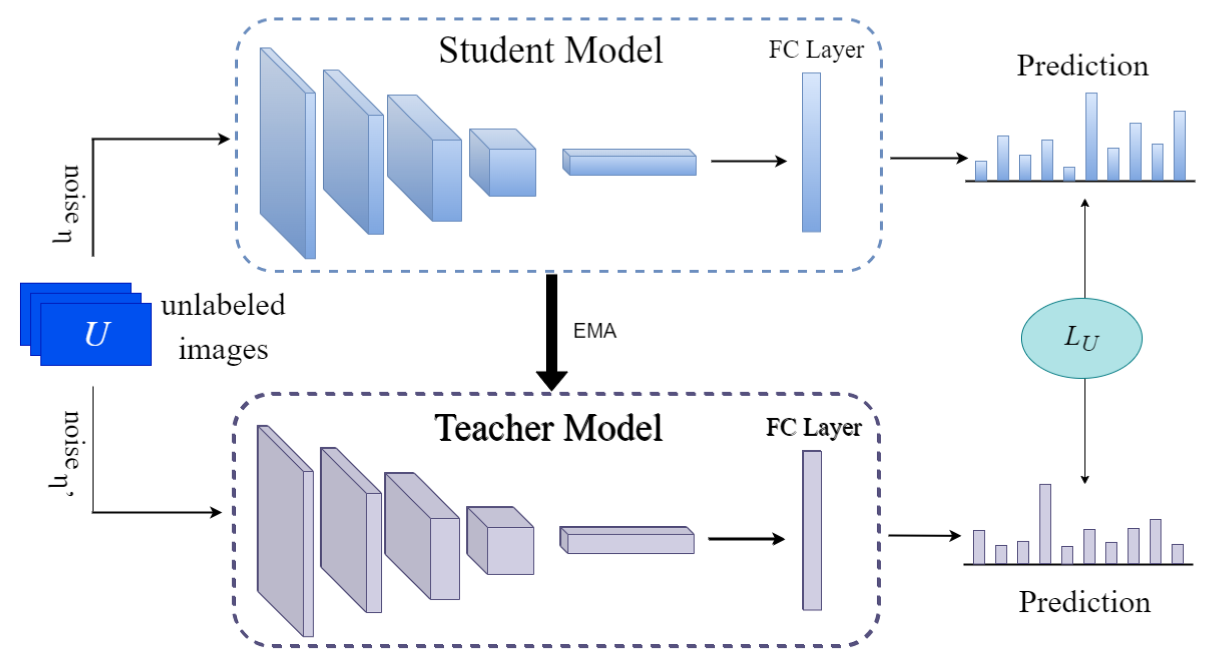
3.3. Unsupervised Losses

As shown in Figure 7, the unsupervised loss in our semi-supervised model is defined as Equation (12).

$${\mathrm{L}}_{\mathrm{IU}}=\{\begin{array}{c}{\mathrm{L}\_\mathrm{w}\times \mathrm{L}}_{\mathrm{U}}{ \mathrm{if} \mathrm{p}}_{\mathrm{t}}{\left(\mathrm{S}\right)=\mathrm{p}}_{\mathrm{t}}\left(\mathrm{T}\right)\\ {\mathrm{H}\_\mathrm{w}\times \mathrm{L}}_{\mathrm{U}} \mathrm{otherwise}\end{array}$$

(12)

where ${\mathrm{p}}_{\mathrm{t}}\left(\mathrm{S}\right)$ and ${\mathrm{p}}_{\mathrm{t}}\left(\mathrm{T}\right)$ are the predicted labels of the samples after the student model and the teacher model, respectively, and the probabilities. Our judgment condition is whether the two predicted labels obtained by the student and teacher models are consistent. $\mathrm{L}\_\mathrm{w}={\left(1-{\mathrm{p}}_{\mathrm{t}}\left(\mathrm{S}\right)\right)}^2$ is the weight that should be given to samples loss judged correctly, and $\mathrm{H}\_\mathrm{w}=1$ is the weight given to samples loss judged incorrectly. ${\mathrm{L}}_{\mathrm{U}}$ is the traditional unsupervised loss, as mentioned in Equation (4). In this way, the model will pay primary attention to the misclassified sample features and allow a more remarkable agreement between the two predicted values obtained from an image.

3.4. Total Model Training Loss

In our approach, the total training loss of the model is defined as Equation (13).

$${\mathrm{L}=(\mathrm{L}}_{\mathrm{C}}{+\mathrm{L}}_{\mathrm{IC}})+\gimel {\mathrm{L}}_{\mathrm{I}\mathrm{U}}$$

(13)

The total loss of our model consists of three components ${\mathrm{L}}_{\mathrm{C}}$, ${\mathrm{L}}_{\mathrm{IU}}$, and ${\mathrm{L}}_{\mathrm{IC}}$, where ${\mathrm{L}}_{\mathrm{C}}$ and ${\mathrm{L}}_{\mathrm{I}\mathrm{U}}$ are obtained by uncertainty weighting the original supervisory loss ${\mathrm{L}}_{\mathrm{S}}$ with the actual unsupervised loss ${\mathrm{L}}_{\mathrm{U}}$, and ${\mathrm{L}}_{\mathrm{IC}}$ is an additional loss used to supplement the supervisory loss ${\mathrm{L}}_{\mathrm{C}}$. $\gimel$ is the parameter used to balance supervised and unsupervised losses.

4. Experiments

In this section, the models are experimented with and compared with previous semi-supervised learning methods [25,26,27,30,31,32,33] on the CIFAR-10 and SVHN datasets, respectively, using different numbers of labeled samples to train our model. The effectiveness of the semi-supervised model can be seen from the experimental results.

4.1. Experimental Parameter Settings

The framework was implemented in Python with the PyTorch library. For a fair comparison, in all experiments, the hyperparameter $\gimel$ was set to 0.1. A conventional SGD optimizer was used with a momentum of 0.9 and a weight decay rate of ${10}^{-4}$. During the training process, the learning rate was set to ${3 \times 10}^{-3}$, and the batch size in the experiments was set to 128. Further, ‘WRN-28-2’ [44] was used as our backbone network. It included leaky ReLU nonlinearity [45] and batch normalization [46].

4.2. CIFAR-10 Dataset

CIFAR-10 [47] is a small dataset for identifying pervasive objects, collated by Hinton’s students Alex Krizhevsky and Ilya Sutskever. It consists of 60,000 32 × 32 colored photographs in 10 categories. Each category contains 6000 images. The size of the images is 32 × 32 (as shown in Figure 8), and there are 50,000 training images and 10,000 test images in the dataset.

As shown in

Table 1. Accuracy of different models using different numbers of CIFAR-10 labeled samples on the test set.

Dataset	CIFAR-10
Labeled	40	250	1000
Pseudo-Label [25]	-	50.22$\pm$0.43	83.91$\pm$0.28
П-Model [26]	-	45.74$\pm$3.87	85.99$\pm$0.38
Mean-Teacher [27]	-	67.68$\pm$2.30	90.81$\pm$0.19
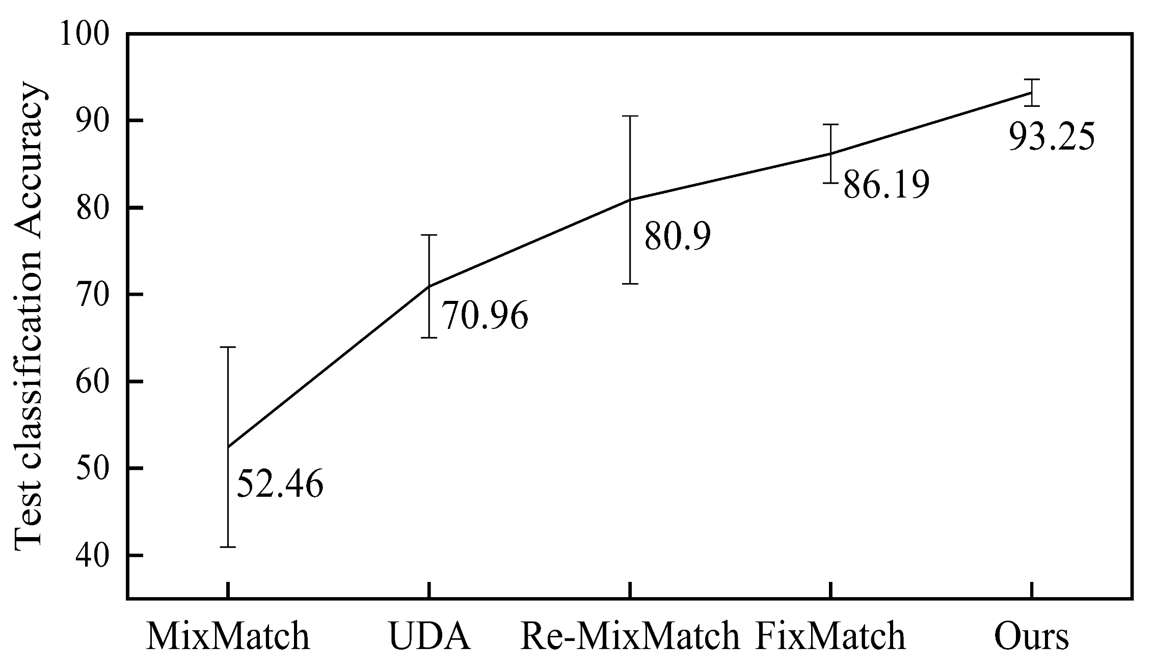
MixMatch [30]	52.46$\pm$11.50	88.95$\pm$0.86	93.58 ± 0.10
UDA [31]	70.95$\pm$5.93	91.18$\pm$ 1.08	95.12$\pm$0.18
Re-MixMatch [32]	80.90$\pm$9.64	94.56$\pm$0.05	95.28$\pm$0.13
FixMatch [33]	86.19$\pm$3.37	94.93$\pm$0.65	95.74$\pm$0.05
Ours	93.25$\pm$1.53	95.38$\pm$0.84	95.96$\pm$0.21

, the model was trained using different numbers of labeled samples and then this method was compared with the previous semi-supervised model. The mean and standard deviation of five runs was recorded. As can be seen, the model shows a significant improvement in accuracy over the previous semi-supervised model on the test set. Specifically, this method improves by 7.06% from earlier when trained with 40 labeled samples. This approach improves by 0.45% and 0.22% over the previous method which used 250 and 1000 labeled samples, respectively.

As shown in Figure 9, it can be seen that this model performs well compared to the previous version with 40 annotated samples from the CIFAR-10 dataset. However, it can be seen from Table 1 that as the number of labeled samples increases, the accuracy of the model improves less and less significantly with the test set. This may be because the previous models have achieved good performance.

Figure 8b shows some artificial samples of CIFAR-10 generated by our model. It can be seen that most of them are clear and have the basic features of each category.

4.3. SVHN Dataset

The SVHN dataset [48] is derived from the Google Street View House Numbers dataset, and each image contained a set of “0–9” Arabic numerals. The training and test sets have 73,257 and 26,032 images, respectively, with an image size of 32 × 32 pixels (as shown in Figure 10).

As shown in

Table 2. Error rates for the test set on the SVHN dataset.

Dataset	SVHN
Labeled	40	250	1000
Pseudo-Label [25]	-	79.79$\pm$1.09	90.06$\pm$0.61
П-Model [26]	-	81.04$\pm$ 1.92	92.46$\pm$0.36
Mean-Teacher [27]	-	96.43$\pm$0.11	96.58$\pm$0.07
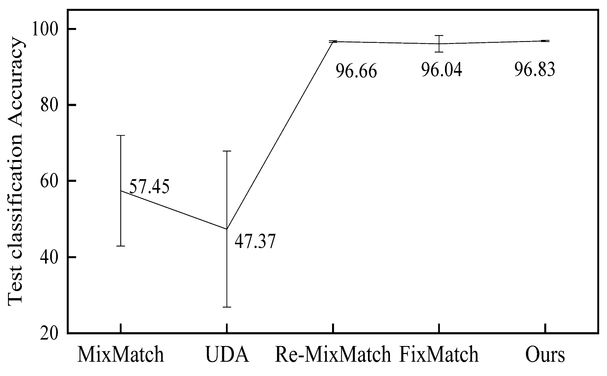
MixMatch [30]	57.45 $\pm$14.53	96.02$\pm$0.23	96.50$\pm$0.28
UDA [31]	47.37$\pm$20.51	94.31$\pm$ 2.76	97.54$\pm$0.24
Re-MixMatch [32]	96.66$\pm$0.20	97.08$\pm$0.48	97.35$\pm$0.08
FixMatch [33]	96.04$\pm$2.17	97.52$\pm$0.38	97.72$\pm$0.11
Ours	96.83$\pm$0.15	97.54$\pm$0.21	97.63$\pm$0.14

, in the SVHN dataset, the model was trained with different numbers of labeled samples and recorded the mean and standard deviation of the five runs of the method. The method improved by 0.79% over the previous method when trained with 40 labeled samples, however, the model does not perform as well in terms of accuracy when trained with 250 and 1000 labeled samples compared to the previous method.

As shown in Figure 11, it can be seen that the model performs well compared with the previous model, which achieved an accuracy of 96.83% on the test set, given that 40 annotated samples from the SVHN dataset were used to train the model.

Figure 10b shows some of the generated SVHN samples with labels, and it is easy to see that most of them are the same as the actual training samples of the SVHN dataset. They have different figures as well as critical features.

5. Discussion

Experiments were conducted on the CIFAR-10 and SVHN datasets to compare them with the existing semi-supervised learning methods. Specifically, the accuracy of the strategy improved on both test sets compared with the current semi-supervised methods. These results suggest that generating some artificial images to supplement the limited number of labeled samples is desirable. Using sample labels as “benchmarks” to compare with labeled sample features in the network complements the original supervised loss and assigns different weights to correctly and incorrectly classified samples, allowing the model to focus more on incorrectly classified sample features. In this way, it is believed that the model parameters can be corrected point-to-point.

However, in the experimental and trial data, a mediocre accuracy performance on the test set was observed when using a more significant number of labeled samples to train the model on both datasets. In the future, more “reliable” artificial samples will be created to improve the performance of the model.

6. Conclusions

A new semi-supervised learning algorithm has been proposed that changes the original supervised and unsupervised losses by assigning weights to different samples to correct the model parameters more accurately. At the same time, the training project generated some artificial examples with labels and mapped the labels as “benchmarks” inside the network to correct the intrinsic feature maps of the labeled samples to learn the sample features more thoroughly and further improve the classification accuracy of the model. A total of 40 labeled samples from the CIFAR-10 and SVHN datasets were used to train the semi-supervised model which achieved accuracies of 93.25% and 96.83%, respectively, illustrating the effectiveness of the proposed method.

References

- Sun, B.Y.; Huang, D.S. Texture classification based on support vector machine and wavelet transform. In Proceedings of the Fifth World Congress on Intelligent Control and Automation (IEEE Cat. No.04EX788), Hangzhou, China, 15–19 June 2004; pp. 1862–1864. [Google Scholar]
- Vailaya, A.; Figueiredo, M.A.; Jain, A.K.; Zhang, H.J. Image classification for content-based indexing. IEEE Trans. Image Process. 2001, 10, 117–130. [Google Scholar] [CrossRef] [Green Version]
- Howard, A.G.; Zhu, M.; Chen, B.; Kalenichenko, D.; Wang, W.; Weyand, T.; Adam, H. Mobilenets: Efficient convolutional neural networks for mobile vision applications. arXiv 2017, arXiv:1704.04861. [Google Scholar]
- Huang, G.; Liu, Z.; Van Der Maaten, L.; Weinberger, K.Q. Densely connected convolutional networks. In Proceedings of the 2017 IEEE Conference on Computer Vision and Pattern Recognition (CVPR), Honolulu, HI, USA, 21–26 July 2017; pp. 4700–4708. [Google Scholar]
- Lin, T.Y.; Dollár, P.; Girshick, R.; He, K.; Hariharan, B.; Belongie, S. Feature pyramid networks for object detection. In Proceedings of the IEEE Conference on Computer Vision and Pattern Recognition, Honolulu, HI, USA, 21–26 July 2017; pp. 2117–2125. [Google Scholar]
- Szegedy, C.; Ioffe, S.; Vanhoucke, V.; Alemi, A.A. Inception-v4, inception-resnet and the impact of residual connections on learning. In Proceedings of the Thirty-First AAAI Conference on Artificial Intelligence, San Francisco, CA, USA, 4–9 February 2017. [Google Scholar]
- Girshick, R. Fast r-cnn. In Proceedings of the IEEE International Conference on Computer Vision, Santiago, Chile, 11–18 December 2015; pp. 1440–1448. [Google Scholar]
- Tripathi, M. Analysis of convolutional neural network based image classification techniques. J. Innov. Image Process. JIIP 2021, 3, 100–117. [Google Scholar] [CrossRef]
- Ning, X.; Tian, W.; Yu, Z.; Li, W.; Bai, X.; Wang, Y. HCFNN: High-order coverage function neural network for image classification. Pattern Recognit. 2022, 131, 108873. [Google Scholar] [CrossRef]
- Minaee, S.; Boykov, Y.Y.; Porikli, F.; Plaza, A.J.; Kehtarnavaz, N.; Terzopoulos, D. Image segmentation using deep learning: A survey. IEEE Trans. Pattern Anal. Mach. Intell. 2021, 44, 3523–3542. [Google Scholar] [CrossRef]
- Hesamian, M.H.; Jia, W.; He, X.; Kennedy, P. Deep learning techniques for medical image segmentation: Achievements and challenges. J. Digit. Imaging 2019, 32, 582–596. [Google Scholar] [CrossRef] [Green Version]
- Zhao, Z.Q.; Zheng, P.; Xu, S.; Wu, X. Object detection with deep learning: A review. IEEE Trans. Neural Netw. Learn. Syst. 2019, 30, 3212–3232. [Google Scholar] [CrossRef] [Green Version]
- Wu, X.; Sahoo, D.; Hoi, S.C.H. Recent advances in deep learning for object detection. Neurocomputing 2020, 396, 39–64. [Google Scholar] [CrossRef] [Green Version]
- Jiao, L.; Zhang, F.; Liu, F.; Yang, S.; Li, L.; Feng, Z.; Qu, R. A survey of deep learning-based object detection. IEEE Access 2019, 7, 128837–128868. [Google Scholar] [CrossRef]
- He, T.; Zhang, Z.; Zhang, H.; Zhang, Z.; Xie, J.; Li, M. Bag of tricks for image classification with convolutional neural networks. In Proceedings of the IEEE/CVF Conference on Computer Vision and Pattern Recognition, Long Beach, CA, USA, 15–20 June 2019; pp. 558–567. [Google Scholar]
- Lu, D.; Weng, Q. A survey of image classification methods and techniques for improving classification performance. Int. J. Remote Sens. 2007, 28, 823–870. [Google Scholar] [CrossRef]
- Wu, J.; Sheng, V.S.; Zhang, J.; Li, H.; Dadakova, T.; Swisher, C.L.; Zhao, P. Multi-label active learning algorithms for image classification: Overview and future promise. ACM Comput. Surv. CSUR 2020, 53, 1–35. [Google Scholar] [CrossRef]
- Rawat, W.; Wang, Z. Deep convolutional neural networks for image classification: A comprehensive review. Neural Comput. 2017, 29, 2352–2449. [Google Scholar] [CrossRef] [PubMed]
- Radford, A.; Metz, L.; Chintala, S. Unsupervised Representation Learning with Deep Convolutional Generative Adversarial Networks. arXiv 2015, arXiv:1511.06434. [Google Scholar]
- Salimans, T.; Goodfellow, I.; Zaremba, W.; Cheung, V.; Radford, A.; Chen, X. Improved Techniques for Training GANs. Adv. Neural Inf. Process. Syst. 2016, 29, 3498. [Google Scholar]
- Imran, A.-A.-Z.; Terzopoulos, D. Multi-adversarial Variational Autoencoder Networks. In Proceedings of the 2019 18th IEEE International Conference On Machine Learning and Applications (ICMLA), Boca Raton, FL, USA, 16–19 December 2019; pp. 777–782. [Google Scholar]
- Wang, L.; Sun, Y.; Wang, Z. CCS-GAN: A semi-supervised generative adversarial network for image classification. Vis. Comput. 2022, 38, 2009–2021. [Google Scholar] [CrossRef]
- Aviles-Rivero, A.I.; Papadakis, N.; Li, R.; Sellars, P.; Fan, Q.; Tan, R.T.; Schönlieb, C.B. GraphXNET—Chest X-Ray Classification under Extreme Minimal Supervision. In Proceedings of the International Conference on Medical Image Computing and Computer-Assisted Intervention, Shenzhen, China, 13–17 October 2019; Springer: Cham, Switzerland, 2019; pp. 504–512. [Google Scholar]
- Jiang, B.; Zhang, Z.; Lin, D.; Tang, J.; Luo, B. Semi-supervised learning with graph learning-convolutional networks. In Proceedings of the IEEE/CVF Conference on Computer Vision and Pattern Recognition, Long Beach, CA, USA, 15–20 June 2019; pp. 11313–11320. [Google Scholar]
- Lee, D.H. Pseudo-label: The simple and efficient semi-supervised learning method for deep neural networks. In Proceedings of the Workshop on Challenges in Representation Learning, ICML, Atlanta, GA, USA, 16–21 June 2013; p. 896. [Google Scholar]
- Laine, S.; Aila, T. Temporal ensembling for semi-supervised learning. arXiv 2016, arXiv:1610.02242. [Google Scholar]
- Tarvainen, A.; Valpola, H. Mean teachers are better role models: Weight-averaged consistency targets improve semi-supervised deep learning results. Adv. Neural Inf. Process. Syst. 2017, 30, 1780. [Google Scholar]
- Miyato, T.; Maeda, S.; Koyama, M.; Ishii, S. Virtual adversarial training: A regularization method for supervised and semi-supervised learning. IEEE Trans. Pattern Anal. Mach. Intell. 2018, 41, 1979–1993. [Google Scholar] [CrossRef] [Green Version]
- Liu, L.; Tan, R.T. Certainty driven consistency loss on multi-teacher networks for semi-supervised learning. Pattern Recognit. 2021, 120, 108140. [Google Scholar] [CrossRef]
- Berthelot, D.; Carlini, N.; Goodfellow, I.; Papernot, N.; Oliver, A.; Raffel, C. Mixmatch: A holistic approach to semi-supervised learning. Adv. Neural Inf. Process. Syst. 2019, 32. [Google Scholar]
- Xie, Q.; Dai, Z.; Hovy, E.; Luong, M.; Le, Q.V. Unsupervised data augmentation for consistency training. Adv. Neural Inf. Process. Syst. 2020, 33, 6256–6268. [Google Scholar]
- Berthelot, D.; Carlini, N.; Cubuk, E.D.; Kurakin, A.; Sohn, K.; Zhang, H.; Raffel, C. Remixmatch: Semi-supervised learning with distribution alignment and augmentation anchoring. arXiv 2019, arXiv:1911.09785. [Google Scholar]
- Sohn, K.; Berthelot, D.; Carlini, N.; Zhang, Z.; Zhang, H.; Raffel, C.A.; Li, C.L. Fixmatch: Simplifying semi-supervised learning with consistency and confidence. Adv. Neural Inf. Process. Syst. 2020, 33, 596–608. [Google Scholar]
- Goodfellow, I.; Pouget-Abadie, J.; Mirza, M.; Xu, B.; Warde-Farley, D.; Ozair, S.; Courville, A.; Bengio, Y. Generative adversarial nets. Adv. Neural Inf. Process. Syst. 2014, 27, 596–608. [Google Scholar]
- Mirza, M.; Osindero, S. Conditional generative adversarial nets. arXiv 2014, arXiv:1411.1784. [Google Scholar]
- Brock, A.; Donahue, J.; Simonyan, K. Large scale GAN training for high fidelity natural image synthesis. arXiv 2018, arXiv:1809.11096. [Google Scholar]
- Odena, A.; Olah, C.; Shlens, C.J. Conditional image synthesis with auxiliary classifier gans. In Proceedings of the International Conference on Machine Learning (PMLR 2017), Sydney, Australia, 15–17 November 2017; pp. 2642–2651. [Google Scholar]
- Lin, T.Y.; Goyal, P.; Girshick, R.; He, K.; Dollár, P. Focal loss for dense object detection. In Proceedings of the IEEE International Conference on Computer Vision, Venice, Italy, 22–29 October 2017; pp. 2980–2988. [Google Scholar]
- Sergievskiy, N.; Ponamarev, A. Reduced focal loss: 1st place solution to xview object detection in satellite imagery. arXiv 2019, arXiv:1903.01347. [Google Scholar]
- Liu, Q.; Yu, L.; Luo, L.; Dou, Q.; Heng, P.A. Semi-supervised medical image classification with relation-driven self-ensembling model. IEEE Trans. Med. Imaging 2020, 39, 3429–3440. [Google Scholar] [CrossRef]
- Zhou, Z.; Lu, C.; Wang, W.; Dang, W.; Gong, K. Semi-Supervised Medical Image Classification Based on Attention and Intrinsic Features of Samples. Appl. Sci. 2022, 12, 6726. [Google Scholar] [CrossRef]
- Haque, A. EC-GAN: Low-Sample Classification using Semi-Supervised Algorithms and GANs (Student Abstract). In Proceedings of the AAAI Conference on Artificial Intelligence, Palo Alto, CA, USA, 22–24 March 2021; Volume 35, pp. 15797–15798. [Google Scholar]
- Li, C.; Xu, K.; Zhu, J.; Liu, J.; Zhang, B. Triple Generative Adversarial Networks. IEEE Trans. Pattern Anal. Mach. Intell. 2021. [Google Scholar] [CrossRef]
- Zagoruyko, S.; Komodakis, N. Wide residual networks. arXiv 2016, arXiv:1605.07146. [Google Scholar]
- Maas, A.L.; Hannun, A.Y.; Ng, A.Y. Rectifier nonlinearities improve neural network acoustic models. Proc. Icml. 2013, 30, 3. [Google Scholar]
- Ioffe, S.; Szegedy, C. Batch normalization: Accelerating deep network training by reducing internal covariate shift. In Proceedings of the International Conference on Machine Learning (PMLR 2015), Hong Kong, China, 20–22 November 2015; pp. 448–456. [Google Scholar]
- Krizhevsky, A.; Nair, V.; Hinton, G. The CIFAR-10 Dataset. 2014, Volume 55. Available online: https://www.cs.toronto.edu/~kriz/cifar.html (accessed on 25 September 2022).
- Netzer, Y.; Wang, T.; Coates, A.; Bissacco, A.; Wu, B.; Ng, A.Y. Reading digits in natural images with unsupervised feature learning. In Proceedings of the Deep Learning and Unsupervised Feature Learning Workshop (NIPS 2011), Granada, Spain, 12–17 November 2011. [Google Scholar]