A Study of Breast Cancer Classification Algorithms by Fusing Machine Learning and Deep Learning

Abstract

Although breast cancer, with easy recurrence and high mortality, has become one of the leading causes of cancer death in women, early and accurate diagnosis of breast cancer can effectively increase the likelihood of a cure. Therefore, it is particularly important to improve the accuracy of early diagnosis of breast cancer. However, conventional early diagnosis relies on human experience and has a low accuracy rate. Therefore, many researchers have proposed various machine learning methods to improve the accuracy and efficiency of prediction. Most of the existing studies around breast cancer classification adopt a single algorithm to fit breast cancer data but ignore the applicability of different breast cancer data features to the model. In this paper, we adopt machine algorithms to strip the features of machine learning methods from the rest of the features and attempt to enhance the model effect by designing deep learning model structures to find the hidden patterns in the rest of the features. In addition, due to strict medical data privacy requirements and high collection difficulty and cost, the model designed in this paper will be trained on a small number of samples. As a result, we attempt to find a minimization model for a breast cancer classification algorithm that features both low cost and high efficiency. At the same time, the deep learning model is further designed to complement the original model when it is possible to introduce complex data indicators. Experimental values show that the design model in this paper performs best not only under limited data and limited indicators but also under limited data complex indicators, demonstrating the effectiveness of the approach of mixed comparison and feature selection of multiple classification algorithms. In summary, the fusion model designed and implemented in this paper performs well in the experiments, and the accuracy of the model test reaches 98.3%.

1. Introduction

Since the middle and end of the 20th century, the global incidence of breast cancer has been rising year by year. According to cancer statistics from the World Health Organization, breast cancer is currently the most life-threatening disease for women, with a prevalence rate of 12.5% in some developed countries. In addition, studies have shown that it is the most diagnosed type of cancer in the world [1]. Although the breast cancer prevalence rate remains low in China, the overall situation is still not optimistic, since the incidence rate and mortality rate of breast cancer among women in China are both higher than the world standard, and worse still, the incidence of breast cancer is increasingly prevalent among the younger population. GLOBOCAN is a significant project of the International Agency for Research on Cancer (IARC), which provides data on incidence, mortality, and cancer trends for 36 types of cancer in 185 countries/regions worldwide. It estimates that the most prevalent cancer among Chinese women is cancer in the breast. As early as eight years ago, in 2009, the Bureau of Disease Control and Prevention of the Ministry of Health of China, in collaboration with the Cancer Center, conducted a detailed data analysis of breast cancer data, suggesting that in regions within China where data have been documented, the incidence rate of breast cancer has jumped to number one, making it the most serious malignancy impeding women’s health. Breast cancer has become the fastest growing cancer in the last decade, with a 37.8% jump in terms of incidence rate over the last decade. Therefore, breast cancer is no longer a health problem for individual patients but rather has invariably become a major public health problem.

Traditionally, a breast cancer tumor is diagnosed by observing the presence of the tumor, the degree of cancer, metastasis location, etc. in a tissue biopsy and pathology section. However, the amount of such data is basically in the order of 10 billion pixels. Therefore, if the number of patients exceeds capacity, the workload of medical staff could become extremely high. In addition, the entire diagnosis process of breast cancer is not only limited by medical levels in different regions but is also easily interfered by the personal, subjective factors of doctors. As science and technology advances, medical data are no longer simply patient information, examination records, etc. Additionally, the data format has also changed radically and morphed into a mixture of video and voice, or a mixture of images and text. Such a complex data model has also become unique to healthcare data. On the one hand, complex data increase the possibility of finding potential causes; on the other hand, however, they increase the cost of medical detection and raise the complexity of algorithms, which in turn makes it difficult to reach the right balance in a limited sample. Under this premise, this paper designs feature selection methods to find the important parts of complex data to construct a minimal medical aid diagnosis model. Furthermore, a well-designed deep learning model is introduced to further tune the minimal medical diagnosis model under the condition of sufficient resources. From the analysis of the experimental results, under limited conditions, the algorithm designed in this paper achieves the optimal effect, the value of the model prediction result (f1_score) reaches 98.24%, the value of recall reaches 98.23%, and the accuracy rate reaches 98.23%. Overall, the overall effect of the model is better than other individual algorithmic models, indicating that in the new development period, it is crucial to apply machine learning techniques in the medical-data-mining segment.

The effective use of medical data requires fast and efficient mathematical methods. The current machine learning and artificial intelligence technologies have advanced dramatically [2]. In the context of the rapid and high development of computer technology, both technologies have been essentially advanced and widely adopted compared to more than a decade ago and have affected all aspects of national society, including national security and people’s daily lives. However, in general, there is still an urgent need for further development and progress of medical data processing methods and artificial intelligence technologies to improve the utilization of massive data in various aspects, integrate information resources, and facilitate more automatic and efficient artificial intelligence. The ultimate goal is to greatly contribute to the progress of national security, people’s lives, and health care. In the process of sampling data from datasets, there are certain errors in the sampling data given the inaccuracy of the experimental instruments, improper procedure management of operators, etc. In the process of measuring the parameters in the samples, individual characteristics of certain sample parameters are not universal. Therefore, we would like to, through an experiment, demonstrate that, under the premise of data screening, it is possible to achieve similar results as by using more data while using parts of the sample data. Such a method not only reduces the computational volume and speeds up the computation, but also paves the way for a further saving of medical resources in the future and for further optimizing the accuracy of the paramedical model by combining the advantages of different data models when more indicators are available.

Medical data is inherently private, and access to it is often costly and requires sophisticated instruments and specialized medical personnel. For paramedical tools that require large amounts of medical data, it is of great interest to achieve essentially the same performance metrics with a very small number of samples compared to the original data. This paper focuses on how to improve the model structure so that the model can still perform very well with extremely small amounts of data. At the same time, the acquisition of any medical metric parameter requires a series of diagnostic methods for judgment, and therefore poses a number of problems:

a)

Increased medical costs. Complex diagnostic methods require more testing costs and experimental costs to determine whether a patient has a disease, which not only increases medical costs for the patient, but also places a huge burden on the patient’s body and mind.

b)

Increased likelihood of error. The testing process of every medical indicator may pose a risk of error because of unpredictable problems in many aspects such as equipment, as well as in medical personnel.

Therefore, reducing the reliance on the number of indicators without reducing the accuracy of the model is highly relevant for breast cancer classification studies. Olfa Hrizi [3] proposes an optimized machine learning-based model that extracts optimal texture features from TB-related images (TB means tuberculosis) and selects the hyper-parameters of the classifiers. However, reducing the reliance on the number of indicators does not mean that a larger number of indicators is less meaningful for paramedicine, but rather that minimal paramedicine, which is the goal of this paper, can be achieved if more desirable results can be achieved with a small number of indicators. In the future, if more detection indicators are available, the judgment effect of the model can be further improved.

Multidirectional diagnosis of breast cancer generates comprehensive and complex data, and the adoption of complex data during diagnosis may lead to two potential effects. On the one hand, the complex data contribute differently to the judgment of the results. While some data can achieve better results using a certain method, other data might not have the same effect using the same method. In this paper, feature selection mechanism is introduced based on this, and different features are fitted using different methods to achieve the best results. On the other hand, the processing of complex data will lead to a geometric increase in the number of model parameters and computational requirements, in which case a small amount of data will easily lead to overfitting of the model. Therefore, this paper designs a feature-splitting mechanism to solve this problem, which proves quite effective as a result. Starting from the techniques applied to breast cancer data determination, machine learning (the method of manually designing feature processing) proves to integrate experience into the model quite well. Yet, for some features where the manual feature-processing approach is not effective, it is important to find the underlying connection of data. In this paper, we adopt a form of convolutional neural network to find this part of the potential connection and attempt to improve the overall performance of the model by combining experience and potential association through model combination.

From the aspect of the model parameter space, fewer numbers of parameters can reduce the decision difficulty of the model. In the case of a larger amount of feature data, the selectable space of each feature will also increase, while the volume of data in the sample will reduce. As a result, it is difficult for the model to learn all the information. In addition, a small relative sample means a sparse feature space, making it difficult for the model to judge sparse data and not easy to fit.

This paper attempts to improve the model, as well as to perform feature selection on the premise of small samples, to make it possible to adopt as few medical indicators as possible to make complementary judgments, and to be able to maintain the original overall medical care level. In addition, to deal with the remaining medical indicators, the paper attempts to further optimize the judgment accuracy by finding potential connections in the data via deep learning methods.

2. Related Work

There are various ways to classify breast cancer; for example, microarray technology [4] analyzes the expression level of thousands of genes simultaneously. Among the available tools for diagnosing cancer, microarray technology has been proven to be effective: classification of triple-negative and non-triple-negative breast cancer patients using a machine learning (ML) approach using gene expression data [5]. In 2020, Elisabetta Rapiti [6] proposed to determine whether the clustering of breast cancer survival is related to patient and tumor characteristics by focusing on histopathological features such as tumor size, lymph node status, etc. The relationship between breast cancer and tumor characteristics has been investigated by immunochemical techniques, and the nature of breast cancer has been explored. In this paper, after scrutinizing its relevance, we chose to explore the characteristics and nature of breast cancer from another perspective, i.e., the accuracy of model fusion in determining the symptoms associated with breast cancer through the relevant techniques of machine learning.

2.1. Machine Learning

Over the last few decades, machine learning has attracted numerous researchers because of its powerful scalability and excellent performance on high-dimensional data. As a branch of artificial intelligence, the basic idea of machine learning is to allow established models to learn from given data to improve their performance. Machine learning can be divided into supervised learning and unsupervised learning. Supervised learning requires that each sample should contain special markers in addition to the feature values. It predicts the markers from the feature values and then compares the actual markers to calculate the error and uses a recursive algorithm to correct the model based on the error. The most common tasks in supervised learning are classification and regression. Unsupervised learning does not require labeling. It explores the degree of similarity between instances or examines the value relationships between features based on specific metrics and methods. The prediction of breast cancer can be seen as a classification problem in supervised learning. A number of machine learning methods have been proposed in much of the literature to help diagnose breast cancer. Dr. Zhou [7] proposed a training model of an artificial neural network (ANN) algorithm using decision tree (DT) algorithm C4.5 by extracting features of various diseases from a routine model. It was found to have high accuracy and also a strong generalization ability. Dr. Huang [2] combined a support vector machine (SVM) with ultrasound texture analysis to classify breast cancer ultrasound images. In 2007, Dr. Wu [8] proposed a cancer prediction model based on the SVM algorithm, which effectively solves the problem of small sample learning and limits overfitting. Dr. Moayedi [9] proposed a three-stage breast cancer diagnosis method with an optimized SVM classifier for classification, and the accuracy of the image dataset could reach 96.6%. In 2017, Dr. Wang [10] used a particle swarm algorithm to select features of high-dimensional mass spectral data, analyzed and compared the results of extreme learning machine (ELM), k-nearest neighbor (KNN), artificial neural network, SVM, and random forest (RF), and, as a result, verified the feasibility of ELM in cancer diagnosis [11]. In 2019, Dr. Miao [12] proposed a machine learning training method based on the spark model and RF with high fault tolerance, fast training speed, and 99.01% accuracy.

2.2. Random Forest

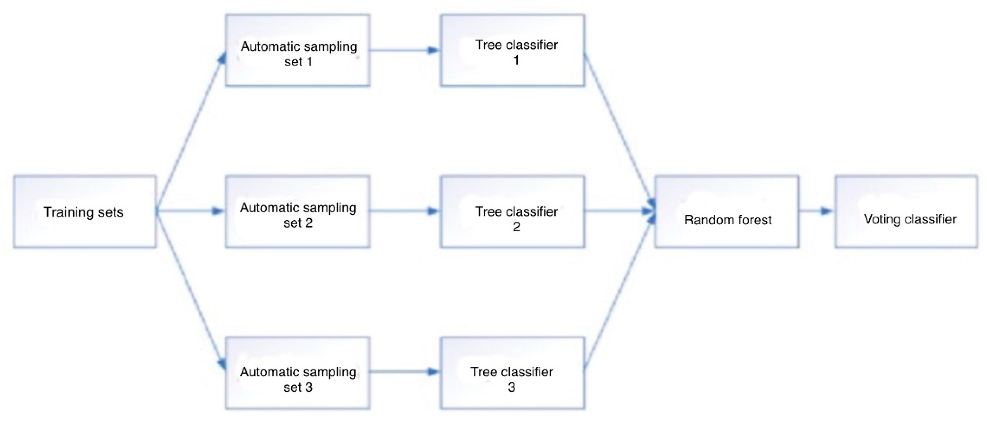
The random forest algorithm is an integrated learning method. In other words, it is composed of many small models and the output of each small model is combined into the final output. The random forest algorithm is a typical machine learning algorithm that is usually adopted to perform classification, regression, or other learning tasks. Based on the bagging algorithm, the random forest algorithm groups data from the original dataset, then trains for each grouping to obtain the corresponding decision tree model, and finally combines and analyzes all the decision data results to get the final random forest model. The final prediction result of the random forest algorithm is based on the voting algorithm, and the classification with the highest number of votes is used as the final output result of the random forest algorithm. The random forest algorithm uses multiple classifiers for voting classification, which can effectively reduce the error of a single classifier and improve the classification accuracy. Compared with the ANN, regression tree, and SVM algorithms, the random forest algorithm has higher stability and robustness, and also leads in terms of the corresponding classification accuracy. The random forest algorithm is good at efficiently processing large-scale data and can be applied to high-dimensional data application scenarios while also maintaining high classification accuracy in scenarios with missing data. Figure 1 shows us the Random Forest algorithm.

2.3. Deep Learning

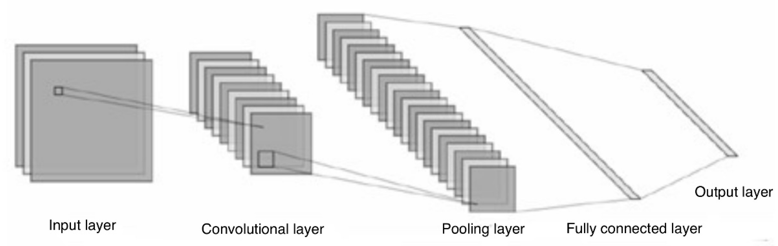
The convolutional neural network is a deep learning method and an important branch of machine learning algorithms. Like a multilayer perceptron of artificial neural networks, it is commonly used to analyze visual images. Convolutional neural networks have long been one of the core algorithms in the field of image recognition and have a consistent performance when learning large amounts of data. The most important features of this network model are self-learning, self-organization, and self-adaptability. For general large-scale image classification problems, convolutional neural networks can be used to build hierarchical classifiers and can also be used in fine classification recognition to extract discriminative features of images for other classifiers. Composed mainly of a convolutional layer and a subsampling layer, convolutional neural networks extract data features for classification by convolution. Specifically, it includes input layer, convolutional layer, pooling layer, nonlinear layer, fully connected layer, classification output layer, etc. Figure 2 below shows the schematic diagram of a convolutional neural network.

As shown in Figure 2, in the convolutional layer of a convolutional neural network model, the input data matrix is first convolved by multiple updatable convolutional kernels, and then undergoes a nonlinear transformation by the activation function, and finally a feature layer is formed. To reduce gradient descent, the activation function of the convolutional neural network model often adopts the ReLu function. After the convolution layer, each output feature map is linked to the original image of the previous input layer by a convolution operation. The convolution process of the convolution layer is as follows.

$${\mathrm{x}}_j^l=f\left({\displaystyle \sum }_{i\in M_j}{x}_i^{l-1}{k}_{ij}^l+b^l\right)$$

(1)

where l is the number of layers of the neural network, k is the convolutional kernel of the network, Mj is the features of the input data, and b is the bias corresponding to the features of each output. The role of the pooling layer in a convolutional neural network is to sample the feature images and obtain their subgraphs. Therefore, it is also referred to as the subsampling layer. If there are m input feature maps after the convolution operation, the number of feature maps remains the same after sampling, which is still m, but the size of the output feature map becomes smaller. The pooling layer is calculated as follows:

$${\mathrm{x}}_j^1=f\left(a_j^l\mathrm{down}\left(x_j^{l-1}\right)+b_j^l\right)$$

(2)

where down (·) is the down-sampling function, which is mainly used to find the maximum or average number in the region for a feature matrix of input size n × n. It is called maximum pooling or average pooling. From the input size, the output feature size is ln of the input data size. A and b in Equation (2) are the biases of the output features. The fully connected and output layers are consistent with the basic neural network structure and the role of the fully connected layer is to expand the feature images sequentially and input the feature information to the neurons. The learning algorithm of the neural network is used to continuously improve the parameters to achieve the best output. In this paper, we mainly adopt a convolutional neural network in data processing and attempt to improve the accuracy of breast cancer classification while optimizing the classification results by improving the classification model.

Currently, automatic breast cancer classification recognition includes both traditional image recognition with manual feature extraction and deep learning-based recognition. Deep learning can automatically extract image features and exclude the human factors in the traditional recognition methods. In recent years, research on breast cancer pathology image classification based on deep learning has developed rapidly, especially the wide application of convolutional neural networks built on large datasets in natural language processing, object recognition, image classification recognition, etc., laying a solid foundation for the application of CNN in breast cancer pathology images. Since Dr. Spanhol and other researchers made public the BreakKHis breast cancer dataset and introduced the pathology image dataset in 2015, a series of research results have been achieved in breast cancer recognition using convolutional neural networks based on this dataset. By adopting six feature descriptions such as local binary pattern (LBP), gray-level co-generative matrix (GLCM), and different classification algorithms such as support vector machine and random forest, the recognition accuracy rate reached 80–85%. Dr. Bayramoglu architected single-task and multi-task convolutional neural networks to predict malignant tumors, increased the recognition rate to 83%, concluded that the recognition rate was independent of the magnification, and, at last, achieved an accuracy rate of 86.3% on breast cancer pathology images. However, the accuracy of the deep learning model for automatic recognition of breast cancer pathology images is not yet as high as expected. Pathological tissue image classification recognition differs from traditional image classification recognition (e.g., recognition of dogs and cats) in terms of image characteristics and dataset size. Pathological tissue images have characteristics such as differential ambiguity, feature diversity, cell overlap phenomenon, and uneven color distribution, especially when the small size of the current pathological tissue image dataset and the uneven number of benign and malignant samples will affect the recognition rate. Therefore, improving the dataset and designing a reasonable learning model, as well as effectively improving the automatic recognition capability, are all important research directions.

3. Introduction to the Experiment

Wisconsin Breast Cancer Dataset

As shown in Figure 3, the breast cancer patient dataset adopted in this paper is from the University of California, Irvine’s machine learning dataset repository, in which the Wisconsin breast cancer dataset was selected.

The goal of this dataset is to predict whether the subject’s breast tumor is benign or malignant, and the dataset is in its original format form, as shown in the following

Table 1. Breast Cancer Data Raw Format.

1	ID	Diagnosis	Mean Radius	Mean Texture	Mean Perimeter	Mean Area	Mean Smoothness	Mean Compactness	Mean Concavity	Mean Concave Points
2	842302	M	17.99	10.38	122.8	1001	0.1184	0.2776	0.3001	0.1471
3	842517	M	20.57	17.77	132.9	1325	0.08474	0.07864	0.0869	0.07017
4	84300903	M	19.69	21.25	130	1203	0.1096	0.1599	0.1974	0.1279
5	84348301	M	11.42	20.38	77.58	386.1	0.1425	0.2839	0.2414	0.1052
6	84358402	M	20.29	14.34	135.1	1297	0.1003	0.1328	0.198	0.1043

.

The features and feature interpretation of this dataset are shown in

Table 2. Dataset feature interpretation.

ID	Number
diagnosis	M = malignant, B = benign
mean radius	radius
mean texture	texture
mean perimeter	perimeter
mean area	area
mean smoothness	smoothness
mean compactness	compactness
mean concavity	concavity
mean concave points	concave points

.

The dataset includes a total of 569 patient data with 32 attributes per patient. The first of these attributes is the patient’s ID number, the second is the diagnosis, and the third through the thirty-second features are computed from digitized images of fine needle aspiration (FNA) of breast masses. These 10 features cover attributes such as radius, texture, perimeter, and symmetry of the cells, and then the variance, maximum, and mean of their nucleus features are calculated separately. Having a multivariate dataset can provide a lot of useful information for data mining, but it will definitely increase the workload of data collection and data analysis. Factor analysis is a statistical method that uses a few factors to reflect most of the information of the original data. Its main steps include correlation testing of the data, factor extraction, naming and interpretation, calculating factor scores and evaluating the sample. In the process of constructing a model, more variables are not better. If ID number is used as a division attribute, 569 nodes will be generated. However, this is not meaningful at all. Therefore, we remove features like ID number and the predicted results. As a result, there are 30 attributes in the remaining dataset, since not every attribute is well-generalized.

4. Methodology

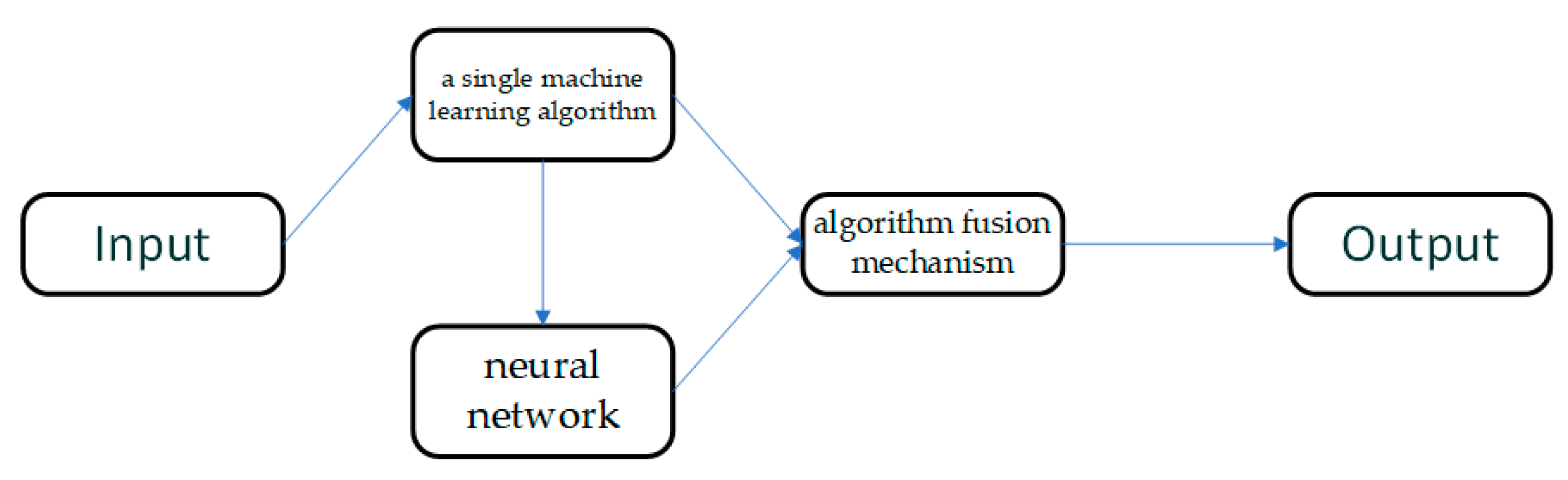
The approach of this paper is divided into three parts. First, a single machine learning algorithm is used to fit the breast cancer data to the limited data available to find regular breast cancer features suitable for use as the basis for machine learning algorithm judgments. Second, a deep learning-based neural network model is designed to learn the remaining features to sort out the distribution patterns behind features that are relatively difficult to train for machine learning. Third, we design an algorithm fusion mechanism to combine the designed machine learning algorithm and deep learning algorithm to improve the performance, as well as stability, of the model.

Figure 4 is used to illustrate the different modules used and the information transformation process:

4.1. Feature Selection Algorithm

To obtain the importance of each feature in the sample, this paper adopts the decision tree method to count the importance of each feature node for the breast cancer classification dataset. To prevent the impact from dividing the samples on the experimental results or the inaccurate feature classification [13], because of individual abnormal sample sets, this paper repeats the experiments by sampling the data several times and training the decision tree separately.

$$C_j=\left(n_0\ast c_0-\sum n_i\ast c_i\right)/T$$

(3)

Shown in Equation (3) is the formula for calculating the degree of importance of each feature (denoted as j) a, where $n_0$ represents the number of statistical samples supporting that feature node, $c_0$ represents the calculated Gini [3] value for that feature node, while $n_i$ and $c_i$ represent the numbers of samples of all sub-nodes of that node and their Gini values, and $T$ is the combined number of samples of the calculated nodes in this formula. $T$ is added to prevent the difference in magnitude caused by the number of samples under different nodes.

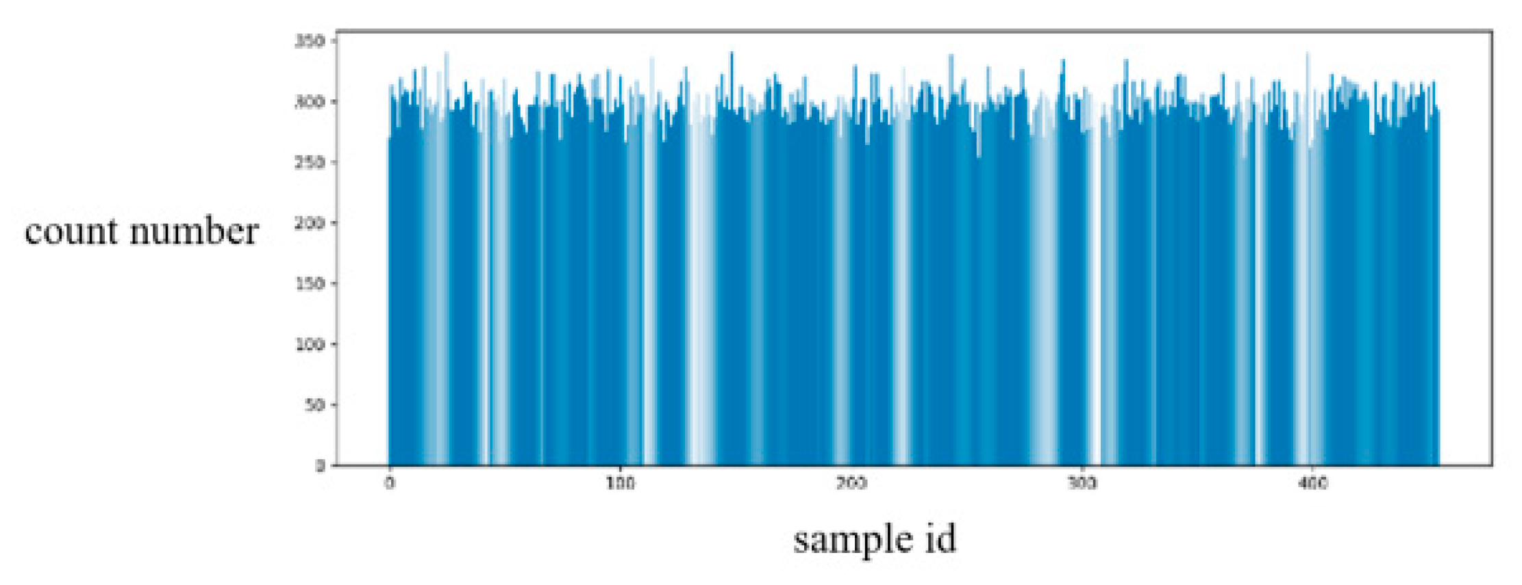
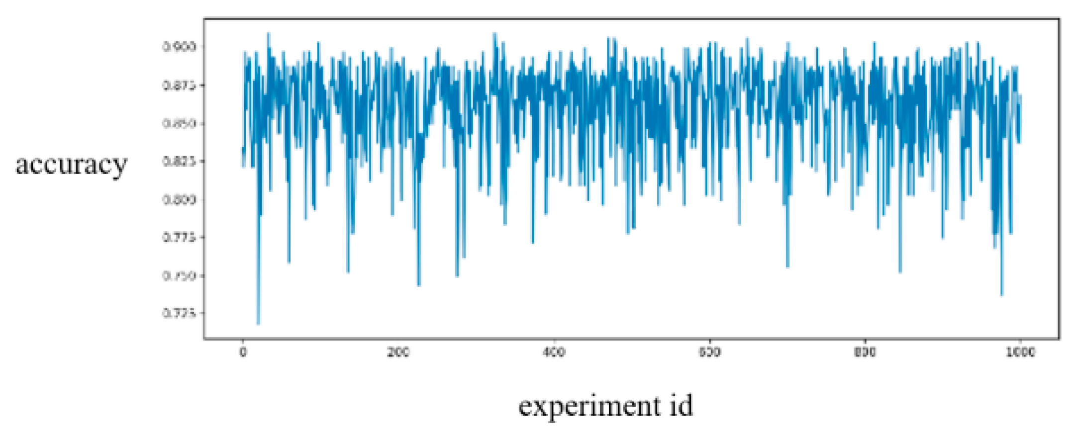
Figure 5 shows the histogram of the number of times each sample was collected after sampling 30% of the samples from the training set as training samples for 1000 times. Figure 6 shows the statistical results of the accuracy of the decision tree trained individually using the 30% of samples obtained from each sampling as training samples.

As shown in Figure 5, the random sampling method in this paper is uniformly distributed sampling and each sample is sampled with approximately equal probability. As shown in Figure 6, 30% of the data are utilized in training, while 70% of the data are used as testing in the training set. The decision tree classification accuracy level proves to be quite high, and its feature weight division value is quite informative (As shown in Figure 7).

In this paper, the experiments explore the performance effect of auxiliary classification models for breast cancer in the case of small-sample experimental data, suggesting that smaller numbers of features reduce the feature dimensionality, prevent the model from fitting the data in unnecessary dimensions, and therefore, reduce overfitting for particular samples. At the same time, since the tree model forms separate branches for each feature dimension, using low-dimensional key features can reduce the complexity of the overall tree structure.

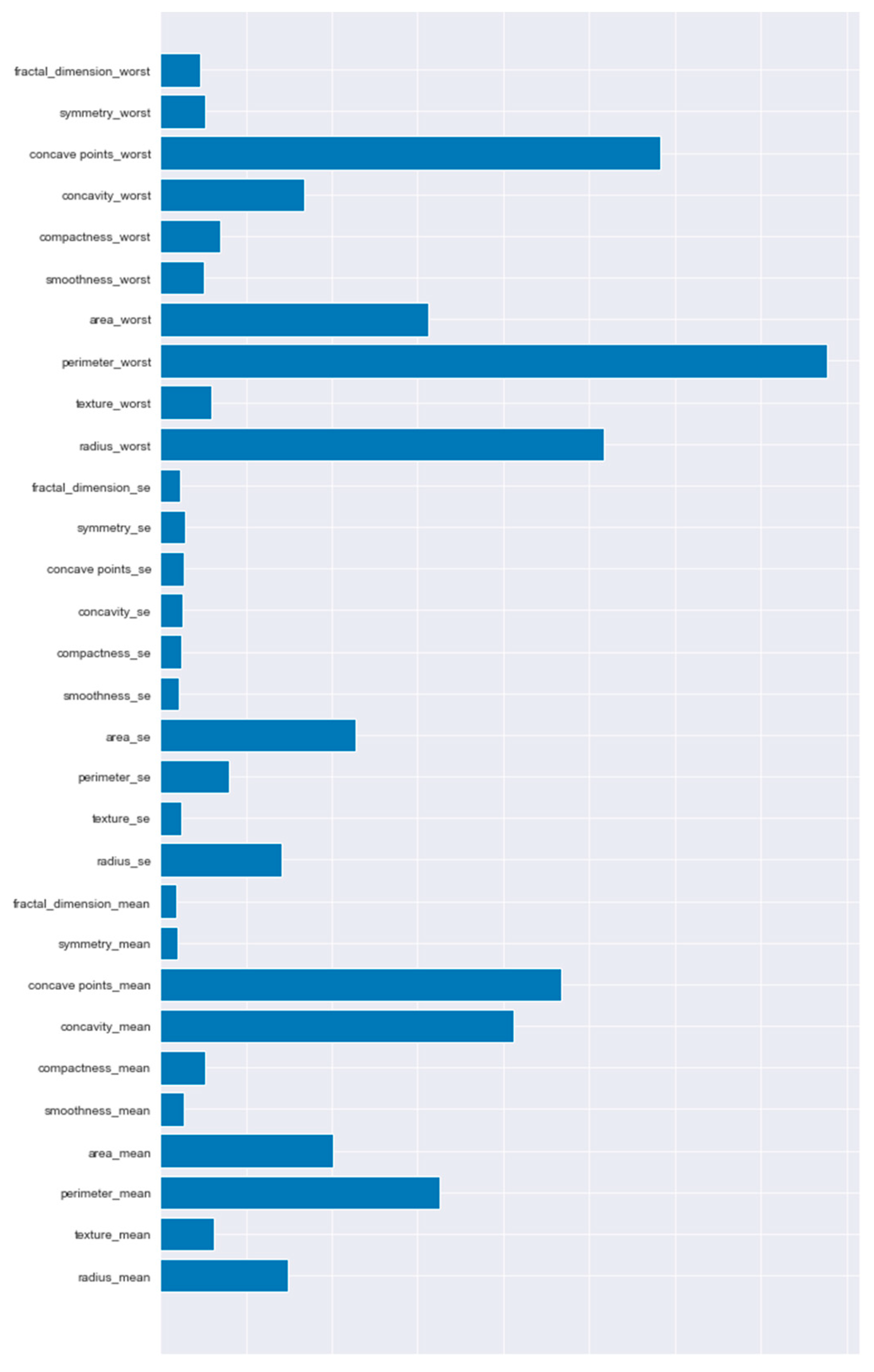
After performing the experiments 1000 times, the importance metric C calculated for each feature was summed to obtain the final importance value for each feature. This value, averaged over multiple samplings, eliminates overfitting errors that may be caused by a single sampling experiment, and the results are more representative of the feature importance profile on the overall dataset. As shown in (Figure 5), features such as cave points_worst, perimeter_worst, radius_worst, cave points_mean, and concavity_mean occupy the vast majority of the information in the data, and these parameters will be used as input to the machine learning model for learning in the following.

4.2. Minimalized Auxiliary Diagnostic Model

Minimalized auxiliary diagnostic model is described with the following equation:

$$\begin{array}{c}S={\omega }_1{M}_{\mathrm{svm}}\left(X^k\right)+{\omega }_2{M}_{rdf}\left(X^k\right)\\ \mathrm{s}.\mathrm{t}{\displaystyle {\displaystyle \sum }_i}{\omega }_i=1\end{array}$$

(4)

where $S$ denotes the final output probability distribution $M_{\mathit{svm} }\left(X^k\right)$ and $M_{rdf}\left(X^k\right)$ denotes the probability outputs of the SVM, random forest, and neural network, respectively. $\omega$ denotes their corresponding weights. Since the actual performance capability of the data is known, we can directly determine the weights based on the data characteristics such as the number of samples and the actual performance. The reason for using a model mechanism that can be very effective against noisy samples, as well as characteristic singleton samples, is that different models have different sensitivities to different kinds of noise, and when a model is affected by a particular sample or noise in it, it can be adjusted by referring to the output of the remaining two models so that the model results do not differ too much from the true density.

The minimalized auxiliary diagnostic model adopts a combination of SVM model and random forest. To achieve the effect of the minimalized auxiliary diagnostic model, the authors chose not to use all 25 features for this part of the model in this paper, but only 5 filtered extracted features, so that the approximate operation of the model can be obtained in a real medical scenario at a faster rate. The accuracy of the model trained with the 5 extracted features will be further discussed below.

4.3. Extraction Neural Network of Feature Hidden Information

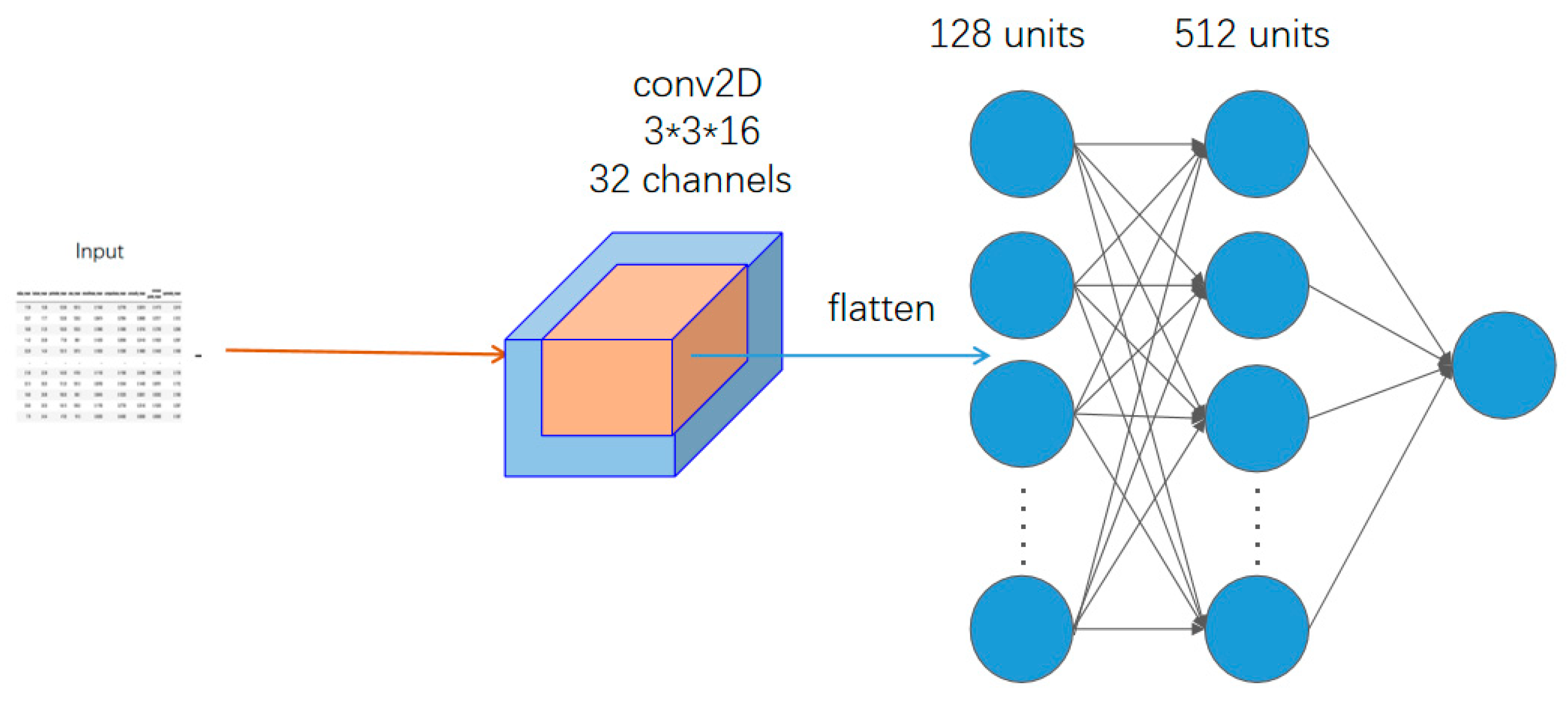
Shown in Figure 8 is a diagram of the overall structure of the neural network designed and implemented in this paper. The overall structure of this neural network can be divided into six layers. The first layer is the input layer, and all the information needed by the model is transferred through the input layer to encode our incoming data as digital signals and then pass them into it. The second layer, the convolutional kernel, adopts 16 3*1*1 convolutional kernels and weights to extract features. The fourth layer and the fifth layer are two layers of the fully connected neural network containing 128 hidden neurons, whose main role is to fit this part of the features after weight extraction. The final layer, the output layer, is responsible for outputting the results of the model.

$${\mathrm{L}}_{\mathrm{e}}=\left({\left({\left({\mathrm{P}}_{\mathrm{f}}-{\mathrm{P}}_{\mathrm{s}}\right)}^2-1\right)}^2\right)$$

(5)

On this basis, this paper introduces the expansion loss, as shown in Equation (5), which helps differentiate the final output probability distribution of the model, and thus reduces the possibility of ambiguous samples in the final result.

$${\mathrm{L}}_{\mathrm{e}}=\alpha \times {\mathrm{L}}_{\mathrm{crossEntropy}}+\left(1-\alpha \right)\times {\mathrm{L}}_{\mathrm{e}}$$

(6)

Shown in Equation (6) is the final loss formula designed and implemented in this paper. A weighting factor $\mathsf{\alpha }$ is introduced in this paper to control the proportional problem of two loss values, where ${\mathrm{L}}_{\mathrm{crossEntropy}}$ represents the base using key features other than those filtered above to get $X^k$ other than the features $X^r$ as the cross-entropy loss function in the neural network training of the input features.

4.4. Model Fusion Algorithm

$X^k$, the breast cancer features with high contribution to the information, are obtained from the above analysis. In the following analysis, $X^r$ will denote the remaining features other than the key features.

$$\begin{array}{c}S={\omega }_1{M}_{\mathit{svm}}\left(X^k\right)+{\omega }_2{M}_{rdf}\left(X^k\right)+{\omega }_3{M}_{nn}\left(X^r\right)\\ \mathrm{s}.\mathrm{t} {\displaystyle {\displaystyle \sum }_i}{\omega }_i=1\end{array}$$

(7)

As shown in Equation (7), the classification distribution of the neural network is extracted by introducing feature hiding information on top of the original minimalized assisted diagnosis model $M_{\mathit{nn}}\left(X^r\right)$. In actual deployment of the model, ${\omega }_3$ will be set to a smaller proportion for optimization. The extraction neural network of feature hidden information is used to fine tune the model output distribution. The main reason is that the core idea of feature segmentation is to optimize the accuracy of the minimalized diagnosis model in the case of small samples, and the idea of model fusion is to give priority to the accuracy and stability of the minimalized auxiliary diagnosis model.

5. Analysis of Indicators

5.1. Evaluation Indicators

Since models often make various changes according to different requirements in real-world application scenarios, we use different evaluation metrics to determine whether the model can function properly under the existing real-world task requirements and environment. Introducing and considering a variety of different evaluation metrics simultaneously when studying real-world problems will be of great help in the model selection exercise conducted in this paper.

In connection with the practical application scenario of this paper, we chose to introduce two different concepts (precision and recall) to assist in solving the relevant problems involved in this paper.

$$\begin{array}{c}\mathrm{Precision}=\frac{\mathit{TP}}{\mathit{TP}+\mathit{FP}}\\ \mathrm{Recall}=\frac{TP}{\mathit{TP}+\mathit{FN}}\end{array}$$

(8)

As shown in Equation (8), precision is mainly based on the actual prediction results of this paper, indicating the proportion of correctly predicted samples in the positive class prediction results. Recall is mainly targeted at the original sample of this paper, indicating the proportion of correctly predicted positive cases in the sample to all positive cases.

After further research, we find that to obtain more-desirable model action results in a practical application setting, in addition to precision and recall, another two quantitative methods, the F1 score and ROC curve, need to be introduced to combine the advantages of precision and recall.

$$\mathrm{F}1=2\ast \frac{\mathrm{precision}\ast \mathrm{recall}}{\mathrm{precision}+\mathrm{recall}}$$

(9)

As shown in Equation (9), the F1 score includes both accuracy and recall in the calculation, helping both indicators to reach the highest point at the same time, maximizing the values of both metrics while maintaining the relative balance between them as much as possible.

$$\begin{array}{c}TPR=\frac{TP}{P}=\frac{TP}{\mathit{TP}+\mathit{FN}}\\ FPR=\frac{FP}{N}=\frac{FP}{\mathit{FP}+\mathit{TN}}=1-TNR\end{array}$$

(10)

As shown in Equation (10), the ROC curve can easily and quickly help discover how well a classifier can analyze the samples at a certain threshold value.

5.2. Cross-Validation

A common method for building models and validating model parameters in machine learning is cross-validation, which generally evaluates the performance of a machine learning model using the data obtained from cross-validation. The basic logic of cross-validation is to select the reused data and the obtained sample data for random classification, first, to form a training set and a test set with different combinations, and then, to formally train the model by predicting the prediction results of the model from the formed training set. By slicing the data in this way, many different test sets and training sets can be obtained, and the samples in the previous test set may become the samples in the next training set, i.e., thus came the concept “crossover”. Figure 9 shows the optimal model mixing ratio derived from the cross-validation method in this paper.

5.3. Analysis of Experimental Indicators

Shown in Figure 9 is a plot of the results of the random forest model when the value of max_features is fixed to control 4 to 5. The max_feature parameter is mainly responsible for controlling the number of features in the selected feature subset. The smaller values of max_feature, the more distinct the trees in the random forest. The horizontal coordinate in the graph denotes n_estimators, which is the maximum number of iterations of weak learners, or the maximum number of weak learners. Numerically, the smaller the value of n_estimators, the more easily the model is underfitted, while the larger the value is, the more easily the model is overfitted. The vertical coordinate is max_depth, which mainly sets the maximum depth of the decision tree in the random forest, and the greater the depth, the easier it is to overfit. Analysis of the data in the figure shows that the model functions optimally when the value of max_depth and the value of n_estimators are maintained in a certain range. The data in the above graph shows that the value of max_features has almost no effect on the accuracy of the random forest model.

Shown in Figure 10 is a heat map of the effect of SVM involving relevant parameters on the model. The horizontal coordinate in the figure is gamma, a parameter that comes with the RBF function after the function is chosen as the kernel. Implicitly, it determines the distribution of the data after it is mapped to the new feature space; the larger the gamma, the more the support vectors; the smaller the gamma value, the more the support vectors. The training and prediction speed of the model receives the effect of the number of support vectors. The vertical coordinate is C, or the penalty function, which represents the tolerance of the model to error. Higher values of C indicate that the model is less tolerant to error and the model is prone to overfitting. Conversely, the lower the value of C, the more likely the model is to be underfitted. Therefore, too large or too small a value of C will affect the generalization ability of the model. The kernel poly in the figure refers to the type of kernel function used in the algorithm. The so-called kernel function is a method used to transform the nonlinear problem encountered by the model into a linear problem. At this point, poly refers to polynomial kernel, kernel rbf (also known as radial basis kernel), and kernel sigmoid (also known as sigmoid function kernel). The overall effect of the model is optimal when the value of gamma, as well as the value of C, is maintained in a certain range.

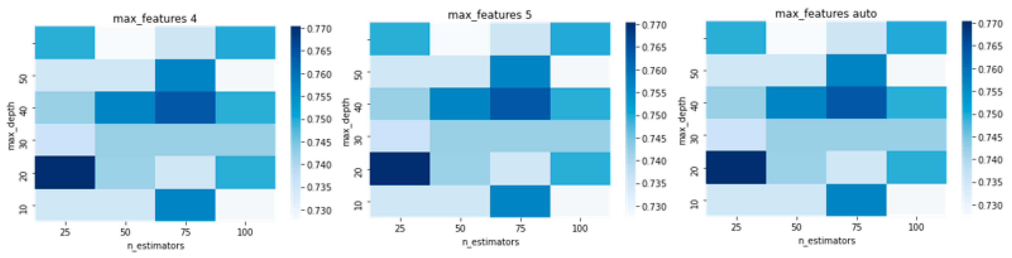
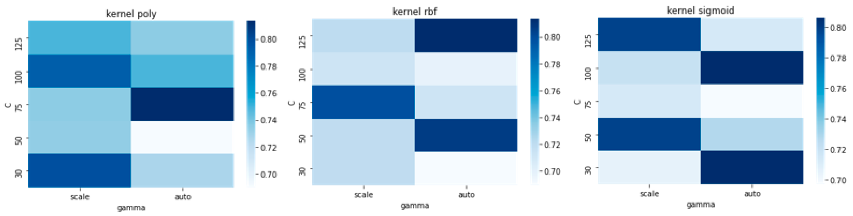
6. Analysis of Results

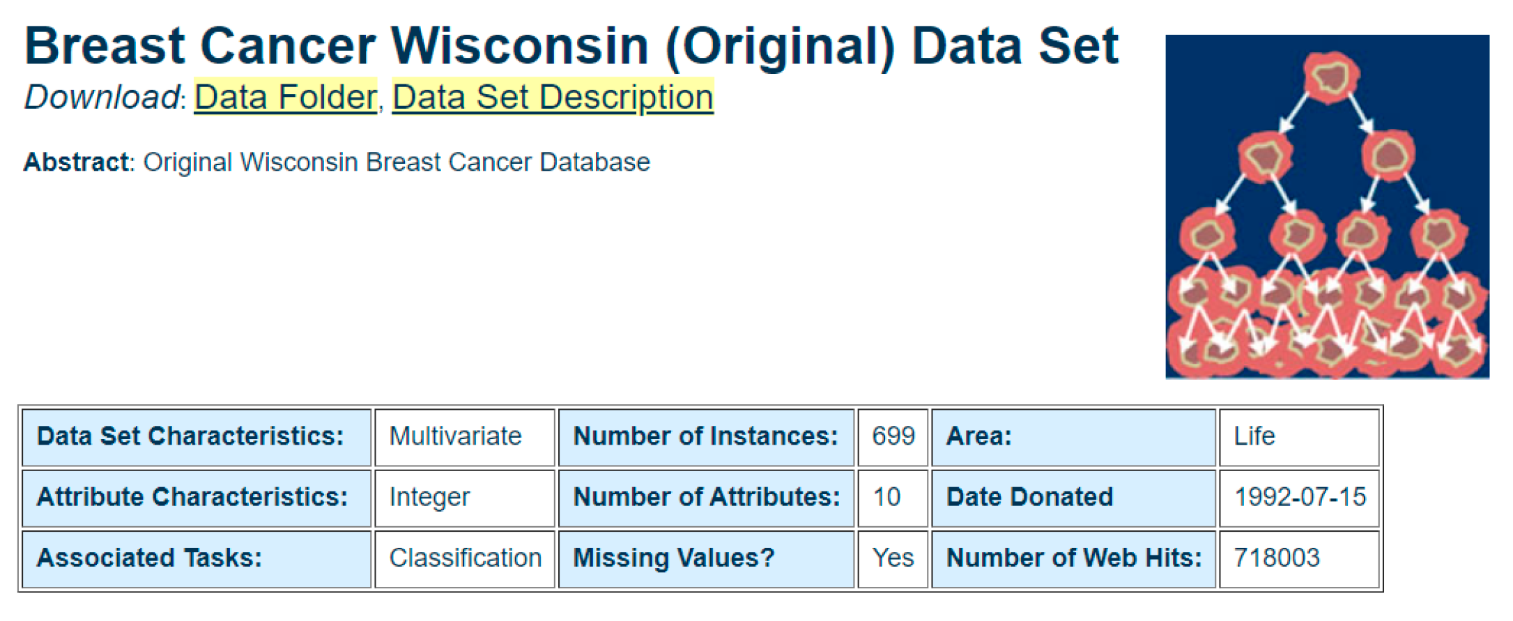
When using the Wisconsin breast cancer dataset as the dataset for this experiment, if the entire data in the dataset are used for model testing, then the accuracy rate can reach close to 100%, whether via random forest or SVM. However, if a small sample of 30% of the data in the dataset are randomly selected for model testing, then the accuracy of the model test drops significantly to 80% using either random forest or SVM. In the case of taking a small 30% of sample data, the data performance of the fusion model designed and implemented in this paper is the same as the performance using 100% data; the better the model accuracy is than the random forest, the better the accuracy of the model when using the random forest and SVM model alone. In the paper “Bayesian network models with decision tree analysis for management of childhood malaria in Malawi” [14], a similar data classification analysis method was used to analyze the related diseases. It used the BN (Bayesian network) model to predict the attributes associated with malaria. The manually created BN model in this article performs significantly better in terms of prediction accuracy but performs slightly worse in terms of f1_score, as well as of recall, compared to the fusion model designed for this study. In a similar comparison, in the article “In comparison, a data-driven approach to a chemotherapy recommendation model based on deep learning for patients with colorectal cancer in Korea” [15], which uses the C3R (colorectal cancer chemotherapy recommender) chemotherapy recommendation model to perform predictive processing of relevant data involved in clinical care, since this model is optimized based on the existing CDSS.

It outperforms some of the other models in terms of model performance, but it still lacks in terms of accuracy and recall when compared with the fusion model designed and implemented in this paper. Shown in

Table 3. Training results for each model taking five extracted features under 30% small sample data.

Method	Accuracy	Recall	f1-Score	Precision
random forest	95.90%	94.02%	91.23%	92.23%
SVM	94.35%	90.35%	90.35%	91.56%
neural network	81.37%	80.76%	81.15%	82.11%
dual-fusion model	98.23%	98.22%	98.23%	98.25%
triple-fusion model	98.24%	98.23%	98.24%	98.26%
BN	97.23%	97.21%	97.23%	97.26%
C3R	97.24%	97.22%	97.21%	97.25%

is data such as accuracy, as well as precision, for training with a 30% data sample using the three models of this paper alone and using the five extracted features for model training. The data in the table shows that the model accuracy of the fusion model and the random forest and SVM reaches 95%, while the neural network model test accuracy is only 80%, which indicates that the neural network is less effective in model training under the condition of small samples, and the model test training has a higher degree of decay and is less stable compared to other models. The models designed in the two articles cited in this paper were able to outperform other single models in this condition in all data; for example, the accuracy BN reached 98.23% and C3R reached 98.24%. In other words, the model prediction effect has been very good. However, compared to the overall performance situation of the fusion model it is still slightly inadequate. In general, the data of each model is relatively smooth, indicating that the model has achieved its best results while having stability, and the test results are representative.

Shown in

Table 4. Training results for each model taking 25 extracted features under 30% small sample data.

Method	Accuracy	Recall	f1-Score	Precision
random forest	93.85%	93.85%	93.88%	94.04%
SVM	93.85%	93.83%	93.84%	93.85%
neural network	96.49%	96.49%	96.50%	96.57%
dual-fusion model	98.24%	98.24%	98.23%	98.23%
triple-fusion model	98.25%	98.24%	98.26%	98.24%
BN	98.24%	98.23%	98.25%	98.24%
C3R	98.23%	98.23%	98.26%	98.23%

is its data, such as accuracy, as well as precision for training using 30% of the data sample with the three models of this paper alone. The models are trained using all 25 features involved in this paper. The data in this table shows that the accuracy and accuracy of the models using all 25 extracted features is reduced compared to the above table using 5 extracted features and the accuracy of the model training for both random forest and SVM is maintained at 91%. The neural network likewise barely performs model training properly using all 25 features, with accuracy remaining at 80%. Under these conditions, the model designed by the article cited in this paper also decreases in effectiveness but still outperforms the other individual models overall. Accuracy rates of 98.24% and 98.23% are achieved for both BN and C3R, respectively, which are slightly worse than the fusion model prediction results. Overall, the data of the models are relatively smooth, indicating that the models have achieved their best results while having stability, and the test results are representative.

Shown in

Table 5. Training results of 25 feature models under all sample data.

Model	Accuracy	Recall	f1-Score	Precision
random forest	95.61%	95.61%	95.63%	95.78%
SVM	96.49%	96.49%	96.51%	96.47%
neural network	98.23%	98.22%	98.21%	98.21%
dual-fusion model	98.24%	98.23%	98.24%	98.24%
triple-fusion model	98.25%	98.24%	98.26%	98.25%
BN	98.24%	98.23%	98.24%	98.25%
C3R	98.23%	98.24%	98.25%	98.24%

is the model training results of the fusion model designed in this paper under all sample data. It is clear from the data in the table that the accuracy of the three individual models, random forest, SVM and neural network, achieves 95%, while the recall and accuracy also remain between 95% and 96% under all the sample data. The training results of the fusion model, on the other hand, are not much different from each of the other individual models and are slightly better than the other individual models, reaching 98.49% in terms of accuracy and maintaining 98.24% in terms of recall, as well as accuracy. The BN and C3R models designed by the two articles cited in this paper achieved 98.24% and 98.23% accuracy, respectively, in this case, and the model prediction results are significantly better than the separate models in this paper. Yet, the overall performance effect was still different from the fusion model designed in this paper. At the same time, the model data fluctuates only slightly, indicating that each model has achieved the best and most stable test effect, and the test results are representative.

Based on the data in the

Table 6. The fusion model designed and implemented in this paper and the test results in two environments with full sample data.

Model	Accuracy	Recall	f1-Score	Precision
fusion model	98.22%	98.21%	98.21%	98.23%
random forest	95.60%	95.62%	95.61%	95.79%
SVM	96.46%	96.39%	96.49%	96.45%
neural network	96.21%	96.22%	96.20%	96.21%
BN	98.10%	98.11%	98.11%	98.10%
C3R	98.11%	98.09%	98.12%	98.11%

, we hereby conclude that the fusion model designed and implemented in this paper tests almost identically in both environments of 30% small sample data and full sample data, and the accuracy is maintained at 98.22% in both cases, while the recall of the fusion model reaches 98.21% and the f1_score reaches 98.21%, compared to the fusion model with only a slight bias in the 30% small sample setting. On the contrary, although the training results of the three individual models of random forest, SVM, and neural network are not much different from the fusion model under the full sample data, the accuracy rate of the three individual models can successfully reach 96.21%. However, the accuracy rate of the model training decays relatively severely under the premise of the small sample data, while the accuracy rate of the neural network model under the small sample environment of 30% can only reach 80%, and the recall rate can also only reach 80.76%, which is a significant decay compared to the 96.21% accuracy of the neural network model in the full sample case. The models designed by the two articles cited in this paper can also maintain some excellent prediction results under the premise of small samples and outperform other individual models, but the results are much worse than the fusion models designed in this paper. At the same time, the data of each model are relatively smooth and the degree of fluctuation is not significant, indicating that each model achieves its optimal effect while successfully having stability and the test results are representative. Therefore, the fusion model designed and implemented in this paper has the obvious advantage of being able to maintain high accuracy, as well as accuracy under small sample conditions, compared to other individual models.

7. Conclusions

This paper focuses on the minimization model in the context of a limited breast cancer dataset. The features that contribute the most to the information of the breast cancer classification model are investigated through a feature selection approach, thus helping to reduce the model parameter space and achieving the minimalized model. A relatively small number of metrics is used to make initial judgments on breast cancer data while achieving more desirable accuracy results. With sufficient experimental resources, this paper, at the same time, investigates the introduction of more metrics to enhance the overall combined performance of the model to achieve the best accuracy results. Future work will investigate more relevant auxiliary diagnostic tools of breast cancer and will combine metrics, as well as image data, for comprehensive multimodal aid diagnosis, while exploring ways to apply the algorithm to other similar diseases.