A Machine Learning Tool to Monitor and Forecast Results from Testing Products in End-of-Line Systems

Abstract

The massive industrialization of products in a factory environment requires testing the product at a stage before its exportation to the sales market. For example, the end-of-line tests at Continental Advanced Antenna contribute to the validation of an antenna’s functionality, a product manufactured by this organization. In addition, the storage of information from the testing process allows the data manipulation through automated machine learning algorithms in search of a beneficial contribution. Studies in this area (automatic learning/machine learning) lead to the search and development of tools designed with objectives such as preventing anomalies in the production line, predictive maintenance, product quality assurance, forecast demand, forecasting safety problems, increasing resources, proactive maintenance, resource scalability, reduced production time, and anomaly detection, isolation, and correction. Once applied to the manufacturing environment, these advantages make the EOL system more productive, reliable, and less time-consuming. This way, a tool is proposed that allows the visualization and previous detection of trends associated with faults in the antenna testing system. Furthermore, it focuses on predicting failures at Continental’s EOL.

1. Introduction

Mass industrialization of products in a factory environment requires product testing before exporting to the sales market. For example, end-of-line (EOL) testing contributes to validating the functionality of an antenna manufactured by Continental Advanced Antenna. In addition, the storage of information from the testing process allows the data to be manipulated by automated learning algorithms in search of a beneficial contribution. Studies in this area lead to the search and development of tools designed with objectives such as preventing production line anomalies, predictive maintenance, product quality assurance, demand forecasting, safety-problem prediction, resource augmentation, proactive maintenance, resource scalability, production time reduction, and anomaly detection, isolation, and correction. When applied to the manufacturing environment, these advantages allow the EOL system to be more productive, reliable, and time-saving.

In this paper, we propose a tool that allows the visualization and early detection of trends associated with the antenna testing system. This tool focuses on the ability to predict failures that occur at the EOL by exploring the data provided from the tests, allowing the user to view graphs which show the progression of the data, as well as predict future data through an artificial intelligence model. The prototype was developed using the Visual Studio Code tool and Python programming language. Google Colab was chosen for model processing.

2. Background

Initially, a survey of the state of the art [1] concerning the problem at hand was conducted, directed at machine learning in EOL testing or the industrial environment. The mentioned paper [1] followed a design science research methodology that revised the necessary technologies to develop the prototype.

Considering the growing demands connected with quality and reliability standards and the vast quantity of data generated by the massive realization of EOL tests, these data can be treated through artificial intelligence/machine learning algorithms [2] to improve industrialization significantly. The survey focused on reviewing the most common machine learning algorithms, which may help develop the system. Out of all the algorithms that were reviewed, long-short term memory networks (LSTM) were shown to be the most suitable based on the generated data.

One application which may be useful to consider can be seen in [3] where Peng et al. used an LSTM model to compensate the negative effects of imperfect channel state information (CSI) in the practical radiofrequency systems. This CSI imperfection is usually caused by the channel estimation error and the transmission and processing delay, knowing that imperfect CSI severely reduces the system secrecy capacity. An LSTM-based predictor was designed to alleviate negative effects effectively.

Analyzing the results obtained from log files (which store the data from testing processes) allows for a better understanding of the evolution of the data, which can indicate patterns and trends based on data sequences (which can be processed by LSTM). Data-driven approaches using machine learning techniques are found to offer a promising potential for improved quality control in manufacturing [4].

Detecting such patterns and trends can help in the preventive detection of system disruptions before a fault occurs in the system or corrective maintenance after detecting a fault in the system.

LSTM is also used for anomaly detection seen in [5]. The cited paper presents a novel detection and prediction procedure based on a LSTM architecture to cooperatively predict process outputs and anomalies by using two separate but interacting models. This interesting application of LSTM allows a solution for short-term as well as long-term anomalies.

Although some applications show the use of LSTM to benefit and optimize the production of certain products, the type of product under study is yet to be seen discussed in other papers.

3. Research Method

Two questions (Q1 and Q2) were formulated, and these two questions guided the review’s objective: to answer both questions and conclude the review. The questions Q1 and Q2 were the following:

Q1:

How do technologies such as machine learning, data science, and deep learning affect the future of EOL testing systems?

Q2:

What are the most impactful applications of these technologies in the manufacturing environment?

Seeking to answer questions Q1 and Q2 allows for the idealization of the problem at hand, aiming to frame some reviewed applications in the antenna production environment, and considering the resources available to carry out the project. This way, it is possible to synthesize the initial problem and explore the alternatives that these technologies’ state of the art has been improving.

Research methodology is a systematic analysis aimed at understanding the method or set of methods to obtain results in a specific task. Typically, research begins with identifying the topic to be tested or studied. Scientific research can be defined as planned research that is based on a specific methodology to contribute to science [6].

The need for a valid research methodology and the same applied to information systems was one of the starting points that led to the development of design science methodology. According to [7], in recent years, the design science methodology has experienced growth due to publicity by various published research works [8,9]. These have included this methodology in the computer systems community as a research paradigm validating its values. The design science methodology consists of creating design theories and/or artifacts to solve a specific problem [10].

Based on reviews of design science research, a design science methodology is proposed based on three research cycles: relevance cycle, design cycle, and rigor cycle [11].

To better understand each of the cycles, the following is a description of each of the cycles individually. The relevance cycle focuses on improving the research environment by introducing new artifacts, thus initiating the design science methodology. It consists of two stages: the first begins with scientific research, where the research requirements are created. After obtaining them, stage two follows, where tests are performed to demonstrate if a correct research artifact was obtained that meets the requirements for solving the proposed problem. If the desired result is not obtained, the cycle must be reformulated with a new research requirement until a satisfactory result is obtained. Subsequently, the design cycle can be defined as the core of the research work, functioning as an artifact generator that allows the evaluation of requirements based on theories and methods extracted from the rigor cycle to achieve a conceivable design. Finally, the rigor cycle is based on the ability to select, interpret, and apply new theories and methods. It is carried out innovatively based on the knowledge of the past to achieve well-founded artifacts and acceptance by the professional audience.

The research presented in this paper follows the design science methodology, where the relevance cycle refers to the basic principles of testing in an EOL environment and technologies in the field of artificial intelligence, the design cycle covers the production of prototypes regarding the intended algorithm, and the rigor cycle includes the studies regarding technologies and forms of applicability and innovation/optimization of mass testing systems. This research methodology solidifies and substantiates the knowledge required to achieve the goal, contributing to the advancement in this field.

The development of the proposed prototype led to a prior literature review, which resulted in writing a paper on machine learning techniques and architectures applied to end-of-line systems, which can be seen in [1]. The mentioned paper reviews some of the most common algorithms applied to EOL systems, thus answering Q1 and Q2, where the obtained answers suggest that some reviewed applications show that it is possible to identify these failures by exploiting data from quality control procedures, selecting the most critical characteristics of the products being manufactured, and identifying patterns related to failures or anomalies. Automatic data processing can be an asset to the test system since the processing of these data ensures that when anomalous samples are encountered, their impact will be reduced.

Based on this information, and as a way to answer question Q1, it can be concluded that the mentioned techniques affect the EOL production/test lines through predictive maintenance, product quality assurance, demand forecasting, safety-issues forecasting, and increased resources. In a specific way, predictive maintenance allows the EOL system to avoid critical equipment downtime with a proactive monitoring of the production line. Furthermore, product quality control tools ensure that production-related problems can be identified early in the production process. Finally, predicting demand for a specific product on EOL systems reduces costs and increases production profits.

Answering question Q2, the most common applications of the mentioned technologies are anomaly detection, isolation and correction, proactive maintenance, resource scalability, and reduced production time. When applied to the manufacturing environment, these advantages allow the EOL system to be more productive, reliable, and with a lower time expenditure.

4. Data Obtained

This section focuses on describing the data obtained, as well as how it was treated and analyzed.

4.1. Data Format

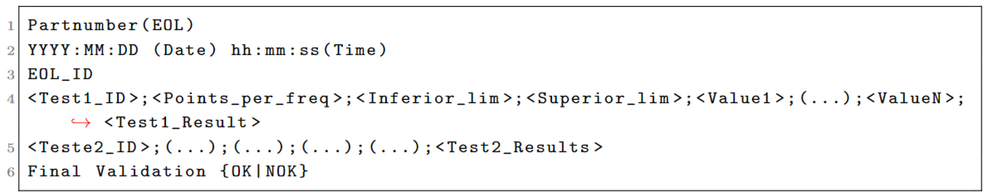
The files represented data from a product (antenna) produced on a manufacturing line, with each file referring to different products. The file information corresponded to the various tests a given product was subjected to during its production or testing. The following Figure 1 shows the basic format of the text files.

The part number (EOL) represents a sequence of standard numbers and letters referring to the manufacturer. This sequence allows one to generate an identification number for the part produced. In the file, one can also identify the data on which the part was tested (line 2) and the name of the final assembly line (line 3) on which the testing process took place. Then, in the file, one can find the tests and their specific characteristics (line 4), submitted to the part on the final assembly line.

The number of points for a given test indicates the frequency signal’s size. The case studies address the tests with one frequency point since the most critical tests are the tests at a specific frequency, therefore testing one value/point in a given frequency range.

Finally, there is the final validation that determines if the piece/product is ready to move on to the next phase of assembly or sale.

Since it is desirable to subject these data to an exploratory analysis for a reflective view of the information, the next step involved using about 5000 files and creating a database (CSV) automatically, in which all the information formatted in rows and columns was appropriately stored. The creation of the database is a fundamental step since it guarantees access to the data in a structured way, facilitating data analysis and exploration.

4.2. Exploratory Data Analysis

After storing the data, the next step was to explore the information contained in the database. A data analysis was performed to visualize the information in a friendly and organized format. The methodology used to perform the analysis resorted to extreme and quartile diagrams, being considered one of the most effective methods for understanding and exposing data in categories [12].

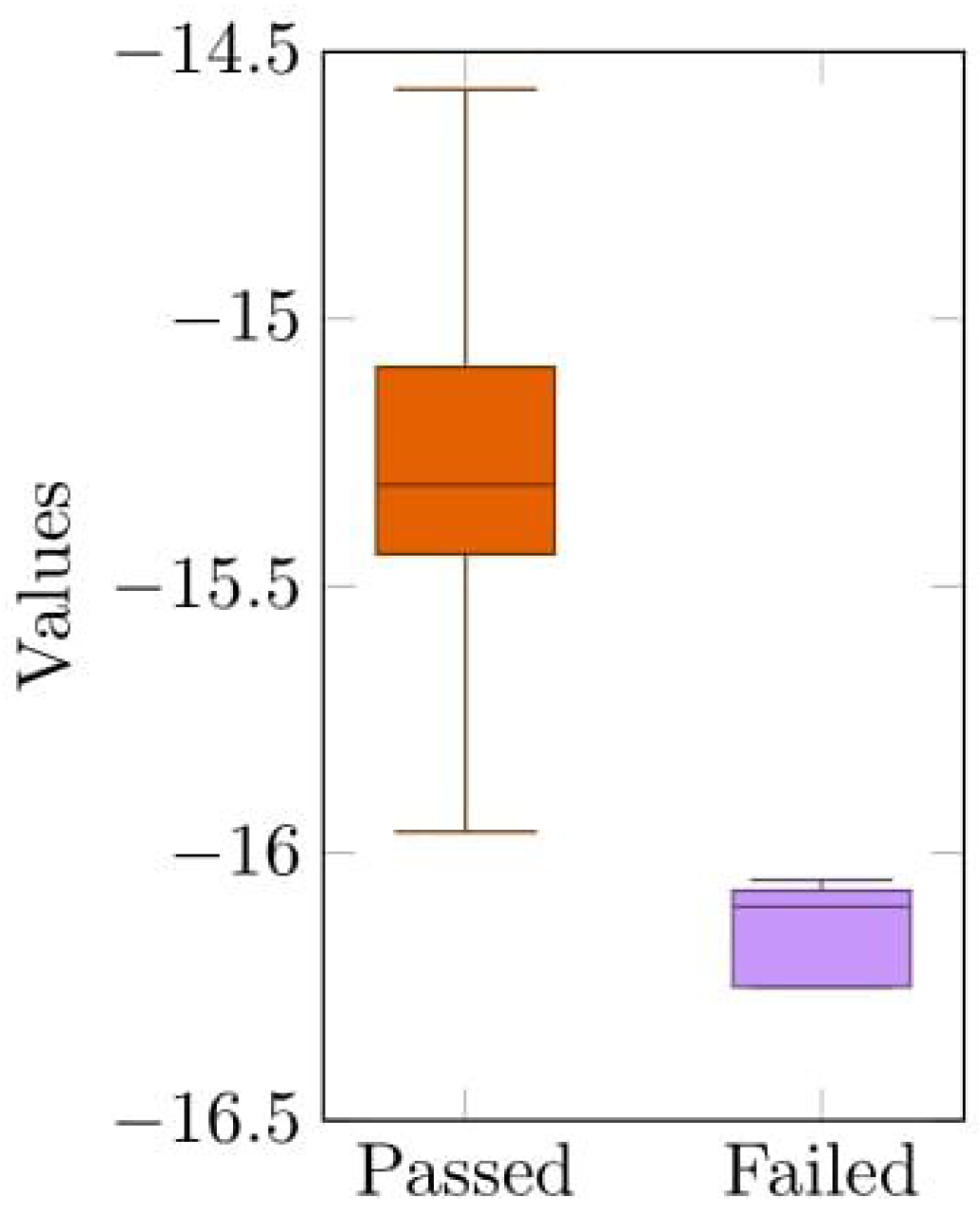
In the context of the problem under study, the diagrams represented the values recorded from the testing for two categories. These two categories were the validated values, or passed, and the nonvalidated values, or failed, that failed in the product-testing process represented, respectively, by the colors orange and purple, Figure 2. The mean, median, first, and third quartile and the maximum and minimum values were calculated to characterize the two categories. The goal at this early stage was to try to break down the different categories in a linear fashion and get a different perspective on the data.

Since the process described allowed us to visualize the differences in values between the edges of the different diagrams, the following section describes the procedure used to calculate a transition value between categories, called a threshold.

4.3. Calculating Thresholds

This section tries to determine a transition threshold between the two classes, looking for the discrimination of value ranges between them.

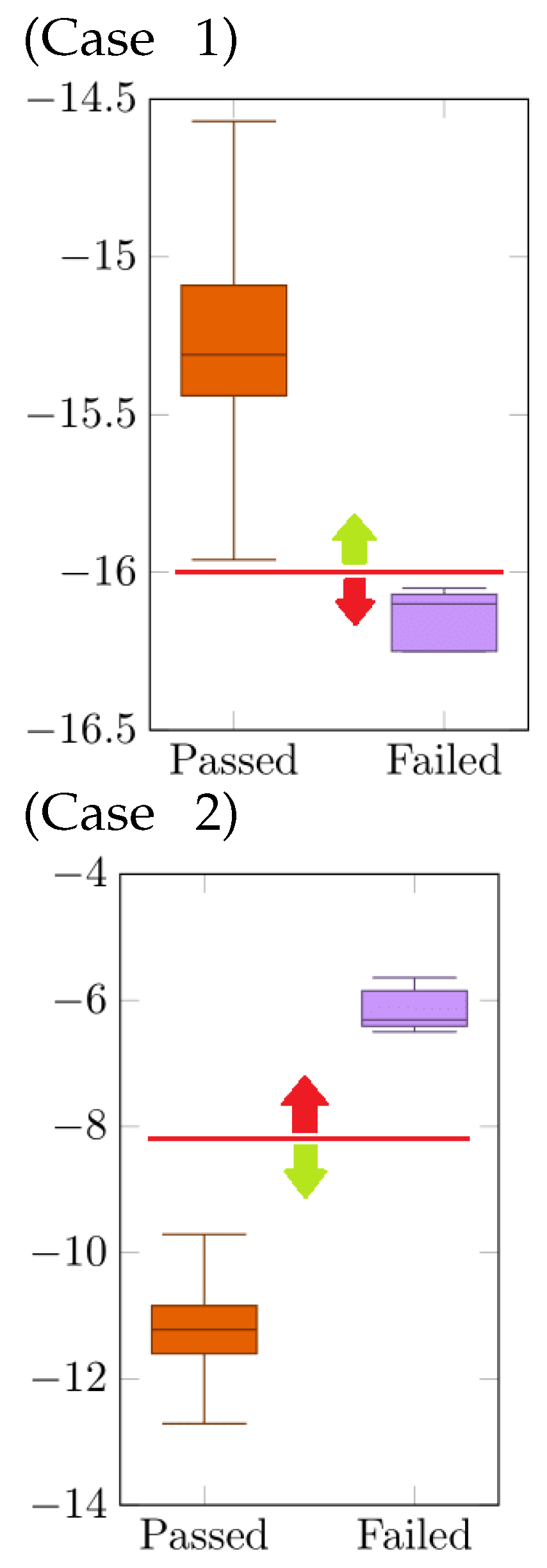
The analysis of the extremes and quartiles diagrams allowed the two classes to be differentiated based on the differences in the extreme values of the diagrams. It was possible to deduce a threshold value or transition between the two distinct categories in the same frequency range for a given test. Figure 3 describes two possible cases, case 1, where the values of the passed category were above the threshold value, and case 2, where the values of the passed category were below the threshold value. This analysis was crucial for the correct monitoring of the values.

The calculation used to determine the thresholds $tr$ relied on the difference between the extremes (lower and upper) of the diagrams of the two classes (passed and failed), divided by two.

$$tr=\frac{{LowerExtreme}_{\mathrm{passed}}+{UpperExtreme}_{\mathrm{failed}}}{2}$$

(1)

4.4. Calculating Confidence Intervals

Confidence intervals [13] represent an estimate of a range of values pertaining to a population of values. This parameter is found through a sample model calculated from the collected data.

The confidence interval is expressed in percentages or confidence levels, with 90%, 95%, and 99% being the most commonly used [14]. In order to calculate the lower and upper limits of the confidence intervals, the following formulas were used:

$$InferiorLimit=\overline{x}-z·\frac{\sigma }{\sqrt{n}}$$

(2)

$$SuperiorLimit=\overline{x}+z·\frac{\sigma }{\sqrt{n}}$$

(3)

Following the formula, $\overline{x}$ is the sample mean value; $\sigma$ is the population’s standard deviation; n represents the sample size; and finally, Z* represents the appropriate value of the normal distribution for the desired confidence level. For the cases illustrated, we had:

$$\mathrm{Z}=1.645, \mathrm{for} 90\% \mathrm{confidence}.$$

$$\mathrm{Z}=1.96, \mathrm{for} 95\% \mathrm{confidence}.$$

$$\mathrm{Z}=2.58, \mathrm{for} 99\% \mathrm{confidence}.$$

The 90%, 95%, and 99% confidence intervals were then calculated, resulting in a total of 3 distinct ranges of CI (confidence intervals), corresponding to degrees of confidence, for each threshold.

5. Comparing Thresholds and Confidence Intervals

Using the thresholds and CI values determined, a method was developed to test the validity of the thresholds and the previously calculated CI from already categorized data.

Testing these values ensure they belong to a transition zone of category values. This method can be integrated into a trend determination in the testing system. It is important to note that the method takes the values of the $passed$ category as a reference because these are the most abundant and represent the default class of tests.

Since building a model requires training and testing phases, it is necessary to split the data. This split used 80% for training and the remaining 20% for validating and testing the logic followed by the model. The data splitting process was performed using a developed algorithm that followed these steps:

• Randomly group all files;
• Create the respective training and test directories;
• Store 80% of the randomly grouped files in the training directory and 20% in the test directory.

The training set is used to obtain the thresholds and CI. That is, with the files in the training directory, the calculations for the training portion of the data are repeated. Initially, the thresholds and CI are read from the training dataset, and a local dictionary is created with this information.

After creating the dictionary and as a way to test the data, the model checks the quality of the thresholds and the CI through the median value of the quartiles coming from the extremes and quartiles diagrams according to the test ID (identifier). In the procedure used, the model assumes that the median is above or below, depending on the case, the threshold limit, or whether or not the median value lies between the defined CI intervals.

Based on this procedure, the model returns a binary vector of labels where values of 0 are considered as the class $passed$ and values of 1 are considered as the class $failed$. This vector, called the prediction vector, is then compared with a vector that has the actual ratings (obtained directly from the text files where the data for an individual antenna are stored). The test directory is traversed to obtain the vector of real values, and if the file presents a failure in any of the tests, the value added to the vector is 1 (positive, that is, the failure is detected). Otherwise, if the file (representative of an individual antenna) does not present any failures, then the value added to the vector is 0 (negative).

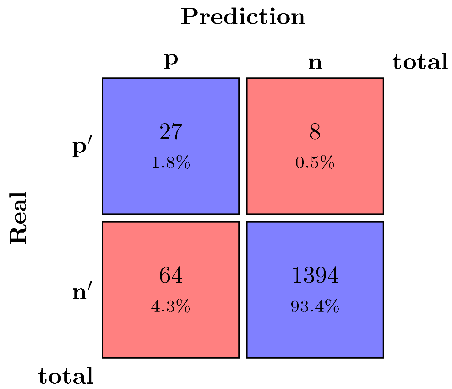
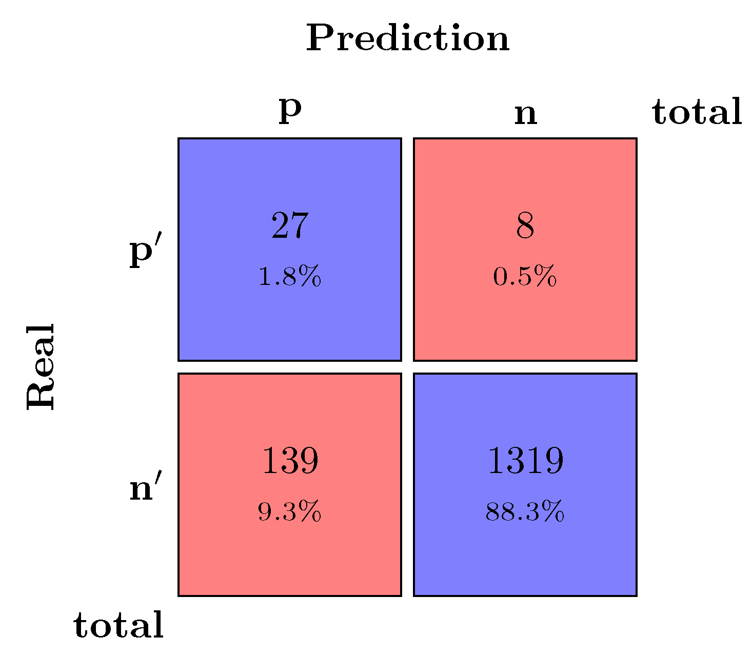
After obtaining the binary vectors of prediction and real values, both were compared, and the confusion matrices are represented in Figure 4 and Figure 5.

Figure 4. Confusion matrix—thresholds.

Figure 4. Confusion matrix—thresholds.

• Accuracy = 0.951;
• Precision = 0.994;
• Balanced accuracy = 0.863;
• Specificity = 0.771;
• Recall = 0.956;
• F1_Score = 0.974.

Figure 5. Confusion matrix—CI 99%.

Figure 5. Confusion matrix—CI 99%.

• Accuracy = 0.901;
• Precision = 0.771;
• Balanced accuracy = 0.578;
• Specificity = 0.993;
• Recall = 0.162;
• F1_Score = 0.268.

The confusion matrices indicate that:

• In the crossing of the first row with the first column are the true positives (the prediction coincides with the actual value, both positive);
• In the crossing of the first row with the second column are the false positives (the prediction does not match the actual value, the prediction indicates that the antenna has had no failures; however, the actual value indicates that the antenna has failed at least one test);
• In the crossing of the second row with the first column are the false negatives (the prediction indicates that the antenna has failed at least one of the tests, but in reality, there are no failures);
• In the crossing of the second row with the second column are the true negatives (the prediction indicates that the antenna has had no faults, and in fact, it does not, coinciding with the real value).

Regarding the confusion matrix of the thresholds model, represented by Figure 4, for balanced accuracy and accuracy, the result indicated that the model performed well, i.e., the procedure of the thresholds model correctly classified most of the antennas. Regarding the precision, the value obtained for the metric reflected a large percentage of correctly classified positive samples. The true positive rate (recall) also resulted in a high value suggesting a low number of false negatives. On the other hand, the true negatives rate (specificity) was the metric with the worst value, which may result in a portion of negative samples predicted even though their true value is positive. The F1_Score metric indicated that the vast majority of positive or negative predictions matched their actual values. On the other hand, the results obtained through the CI confusion matrix represented by Figure 5 were not as good as those of the previous thresholds model. There was a sharp decrease in the metrics balanced accuracy, recall, and f1_score. The values of these metrics were changed due to a more significant number of false negatives and less true negatives.

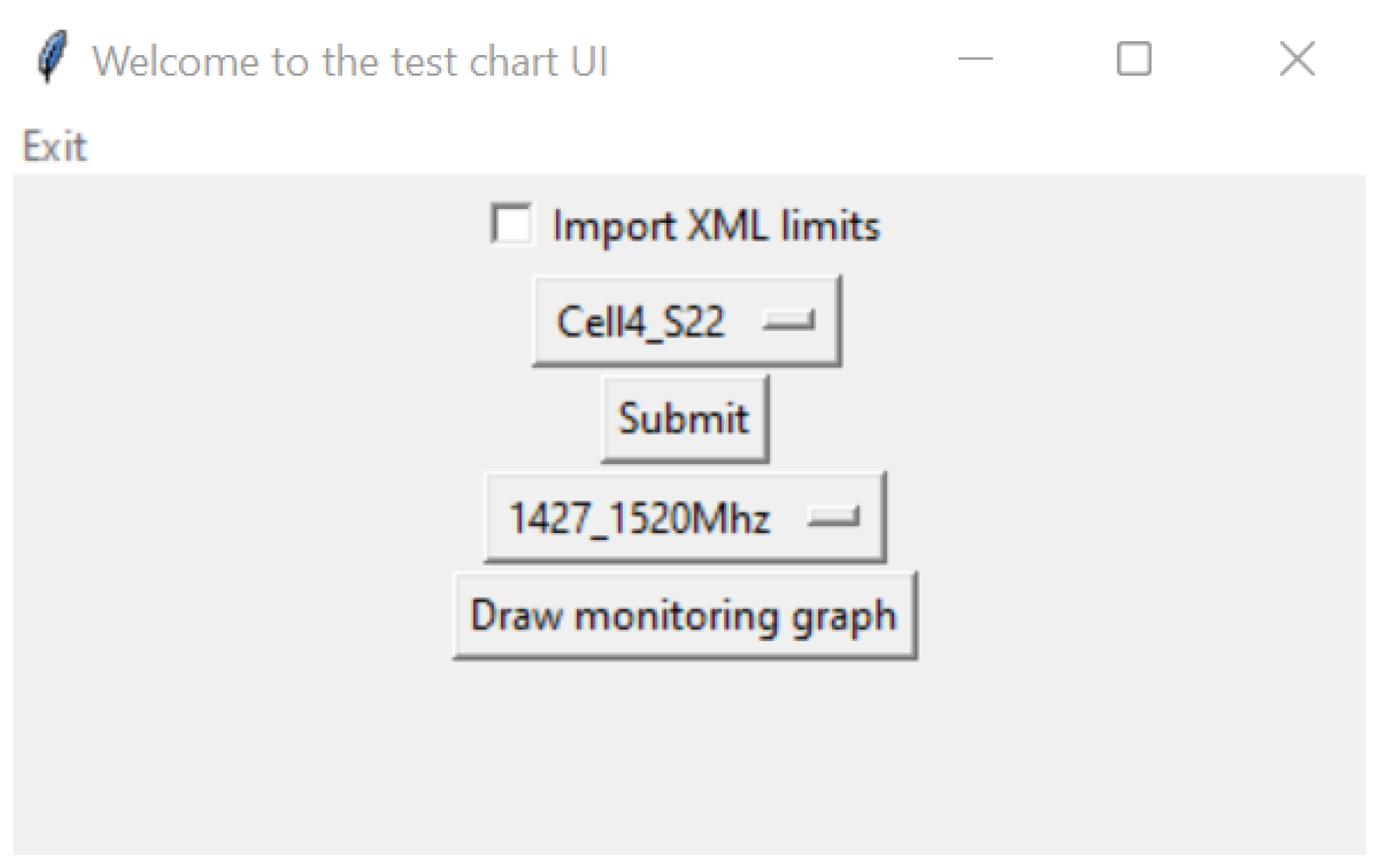
6. User Interface

This section describes a user interface developed to interact with the algorithm for trend monitoring.

The developed interface consists only of buttons and a selection box. Therefore, the user can select the test they want to view. The list of tests is in the selection box (Figure 6). The graphical interface was developed using the Tkinter library. As previously stated, each test has its critical frequency points, so after choosing the test, the user must submit the frequency range (Figure 7).

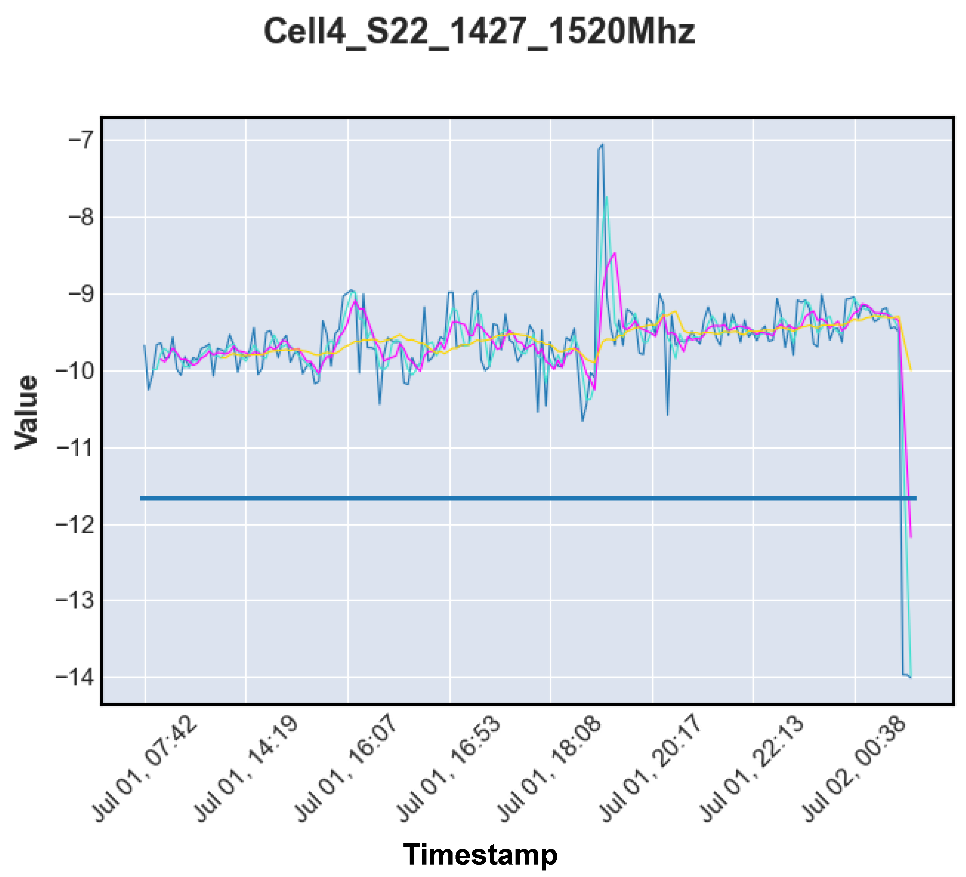
In order to obtain a graph, the algorithm collects data from an SQL database where the test results are stored in real time (connected to the assembly line), after obtaining the data through an SQL query with the base format for drawing the graph. By default, the algorithm uses the calculated thresholds to complement the graph, and this is the value that determines if the test is close to a zone indicative of a tendency to fail or not.

Figure 8 shows the result of a possible test, as well as the said threshold value in blue color. The graph illustrates the evolution of the values tested in the Cell4_S22 test in the frequency range 1427–1520 MHz by various antennas over a time span represented by the abscissa axis. The graph is also complemented by moving averages that represent an average estimate of the values tested by sequential samples.

Trend Monitoring

The system detects that the antenna test results deviate from typical values when one of the moving average indicators exceeds the defined threshold value. In this case, the user is notified of the occurrence of an alarm displayed in the application. This procedure is based on the fact that these indicators are directly related to the represented values, so if one of the moving averages exceeds the defined thresholds, it means that there was a number of undesirable values outside the normal range. The algorithm generates three types of warnings, depending on the moving-average curve that exceeds the outlined limits (Figure 8):

• The cyan-blue moving-average curve represents the curve with the highest volatility as it considers sets of three past values to calculate the arithmetic mean and is the most influential curve.
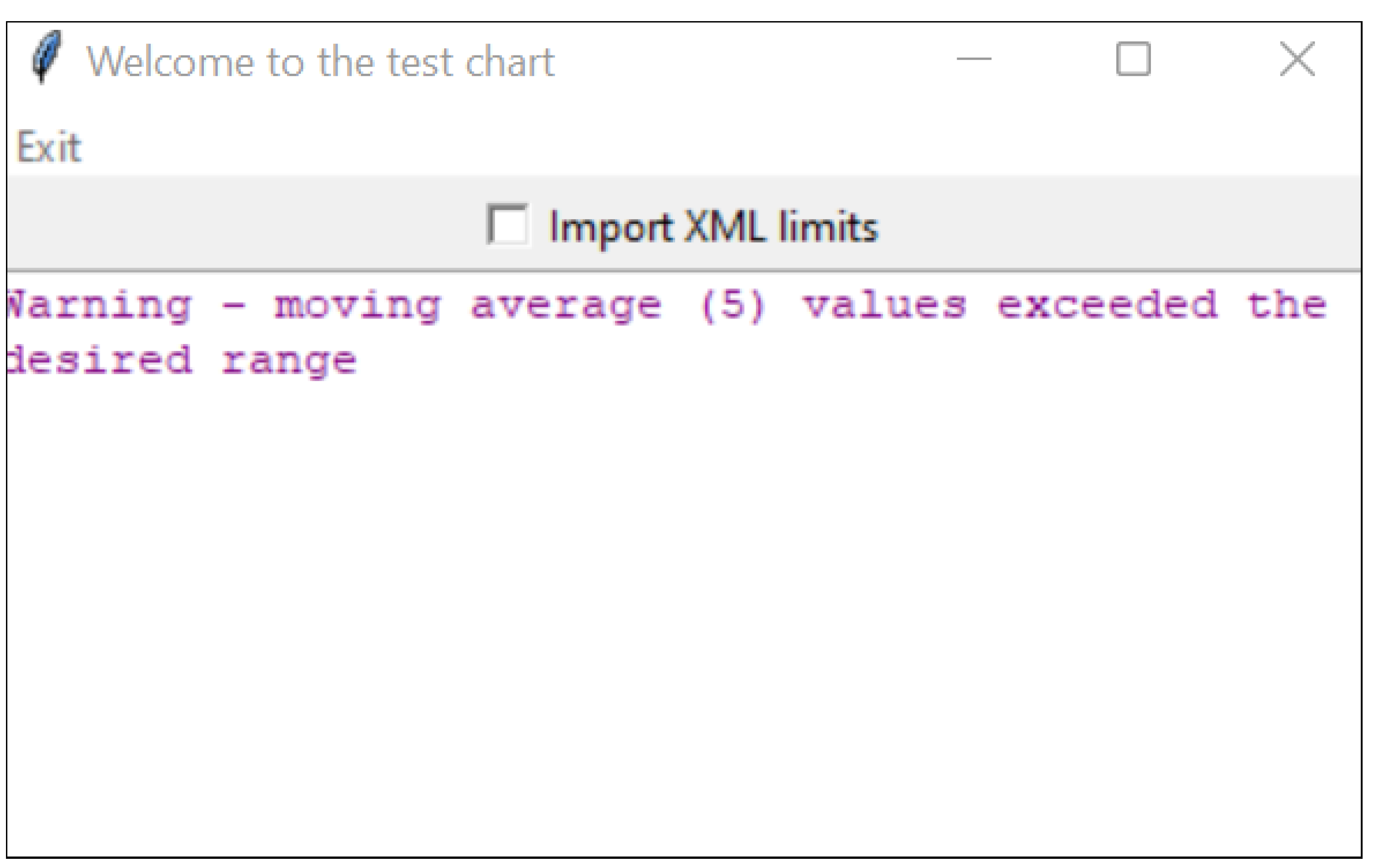
• The purple curve represents the average volatility and considers sets of five past values to calculate the average, and a medium concern alarm is triggered.
• The yellow curve represents the least volatile moving average considering sets of twenty past values for calculating the average being the least influential, requiring a more significant number of values outside the expected limits to be considered a trend. It represents the most severe alarm.

Alternatively, if the algorithm does not register any abnormality in the data, it returns a message suggesting that everything conforms with the expected values. For the case under study, the user interface generated the warning represented by Figure 9. This type of monitoring applies the analytical tool of creating manufacturing sustainability [15].

Although the application developed allows a detailed analysis of the behavior of the values tested on the assembly line complemented by feedback through different alarms based on the graphical behavior, the last part of this manuscript focuses on the development of a system capable of predicting the behavior of the values tested. A system capable of predicting the system’s future behavior becomes necessary since the algorithm developed for the graphical interface needs the data to be stored in the database to conclude whether there is a trend, which means that the said trend may already be occurring. The following section uses an LSTM model to predict, based on past data, the behavior of the assembly line.

7. Forecasting Results with the Use of an LSTM Network

The test results were indexed by a temporal range of values represented by the $yy$ axis (the values from the tests). There was a correspondence on the $xx$ axis representing the date on which that value was recorded. In this way, the data allowed the use of an LSTM network capable of making predictions by studying sequences of values.

However, in order to constitute a prediction, this type of analysis must be based on future events to incorporate and project data related to the past in a predetermined and systematic way. In order to obtain a prediction on this type of data, the model must be able to interpret various sequences belonging to the data set already on record and project the appropriate prediction of future values. Next, we present the methodology used to fulfill the proposed objective, as well as the conclusions.

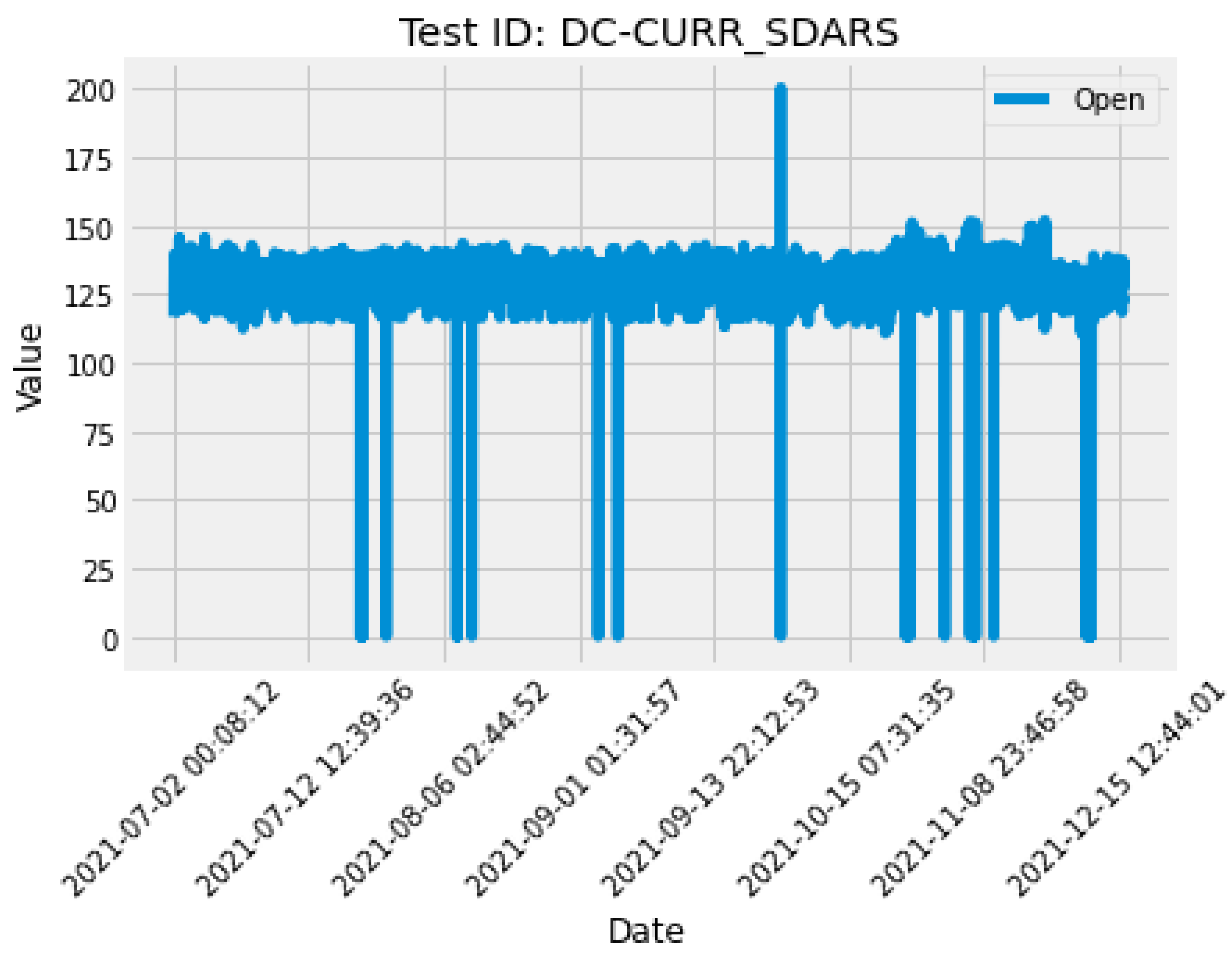
The graph represented by Figure 10 illustrates the DC-CURR_SDARS test over a time range of approximately five months.

After transforming the data, the next step involved selecting seventy percent of the data for a training dataset and the remaining thirty percent for a test dataset. The methodology used for creating the variables x_train and y_train considered sequences of 100 elements for x_train and element 101, i.e., the element following the sequence of the one hundred selected elements, was stored in y_train, representing the desired value that the model should achieve (or the prediction). The same applied to the test variables. The arrangement of the data and proper organization of these training and test variables allowed the data to be formatted for network training.

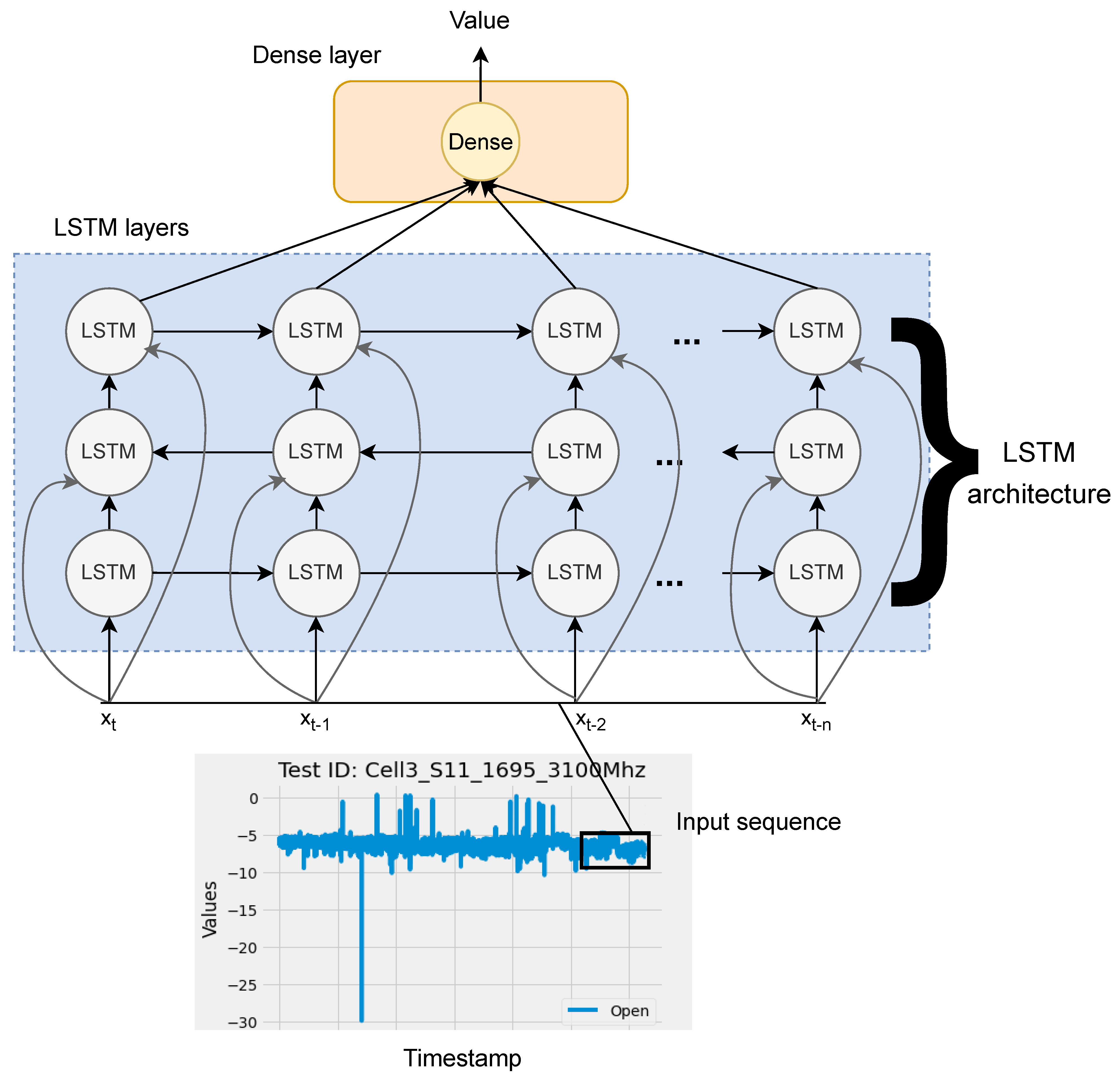
Using the Keras library [16], the model was built by three LSTM layers (fifty units each) and a dense layer (with one neuron), see Figure 11.

After adequately inserting the training variables into the model and the test variables as validation, the model was trained for six seasons.

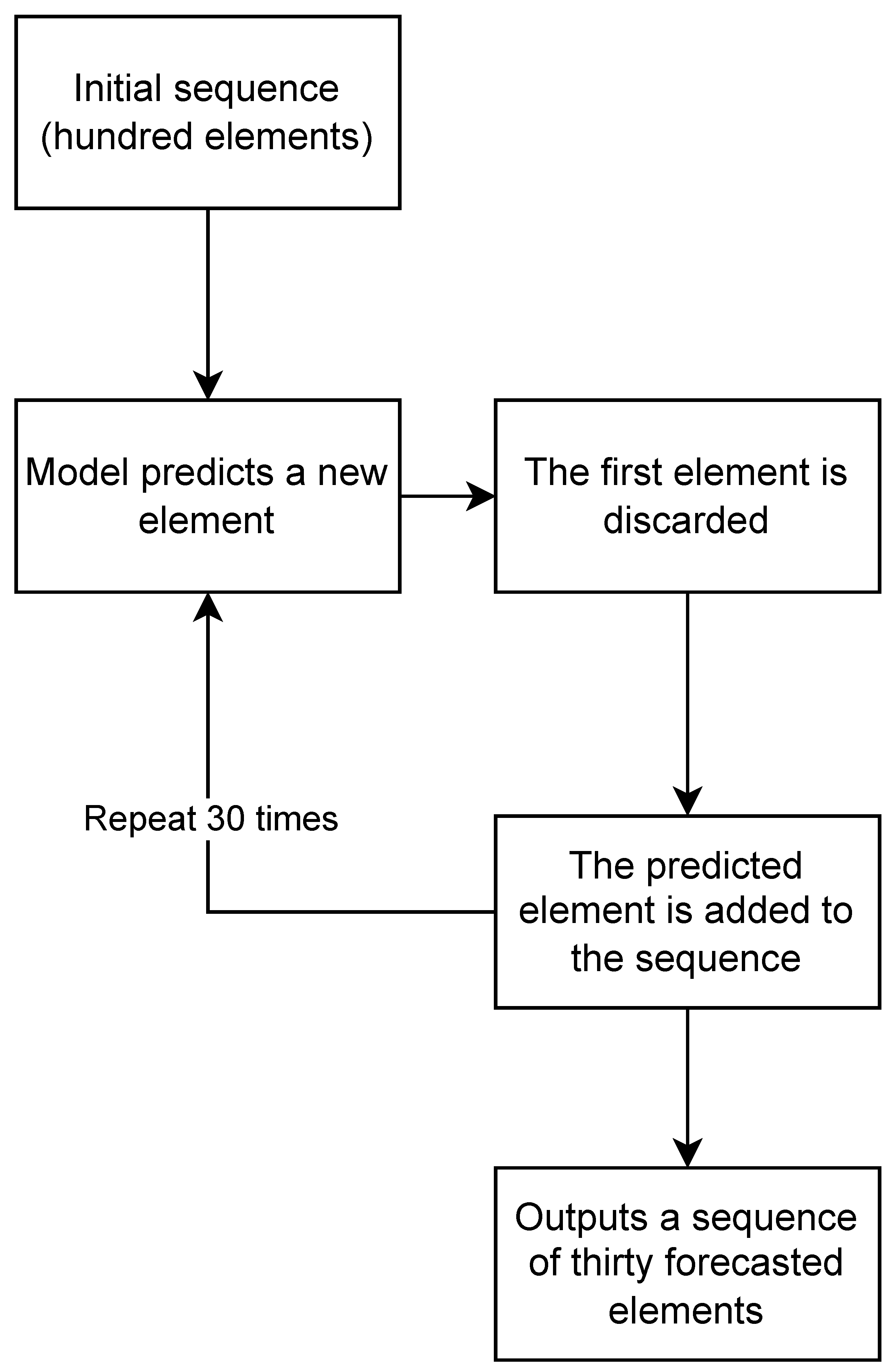
Although the model had an acceptable accuracy, it could not be assured that these were predictions that projected the behavior of future values. The behavior of the predictions obtained followed the data represented. However, it did not guarantee how future behavior would look like, so the next step involved obtaining a prediction that suggested the behavior of the next 30 antennas to be recorded. To make this possible, the sequence of 100 antennas to be considered was the last 100 antennas recorded in the test dataset.

The model then considered the input sequence of 100 elements and predicted element 101. The first element of the sequence was removed, and the predicted element (the one with index 101) was added to the end of the sequence generating a new sequence of 100 values for the next iteration. This process was repeated 30 times until the desired sequence of 30 elements was obtained, see Figure 12.

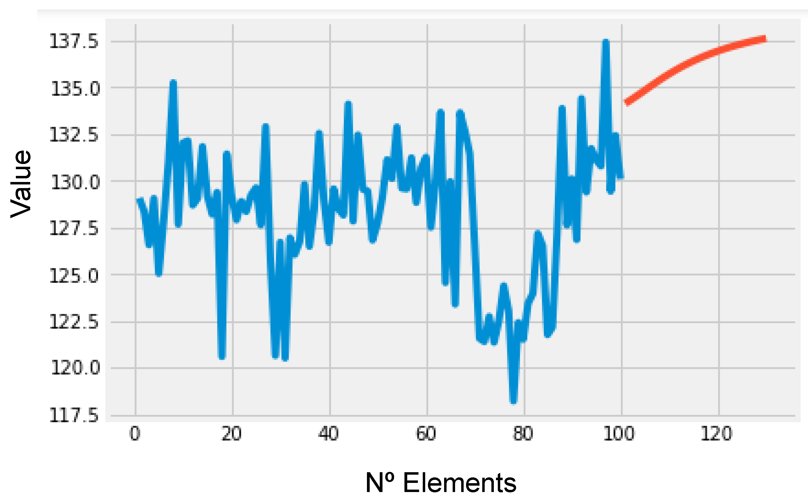
Finally, after the 30 iterations, the result was placed on the graph along with the sequence considered in the first iteration. The reason we stuck with 30 iterations was because it felt like the “safe zone”; this number of iterations could be higher, although it could hurt the performance of the algorithm and make it biased. A higher number of iterations could result in having a sequence used to predict new values (100), where more than a third of its elements (30) would already be a prediction, which means the model would be doing predictions based on predictions. As such, the goal was to then validate the prediction and keep training the model once the forecasted values were validated; this way, we ensured that at least two thirds of the data were real and not forecasted.

Figure 13 displays the prediction result (red color) as well as the initial value sequence (blue color). This type of usage allows the LSTM network to play the role of predictive maintenance. This model could be applied to seek this type of task in industry, playing a useful role which can support workers to carry out equipment maintenance [17,18].

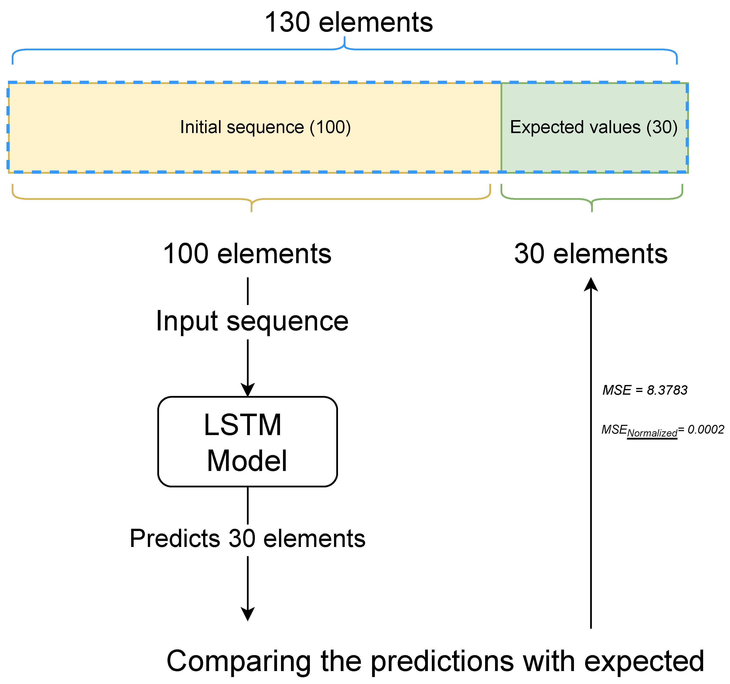
Validating the Model

In order to verify the veracity of the prediction obtained by the model, an initial sequence of 130 values was stored in the database before the prediction was made. Of these 130 values, the last 30 values were stored separately, to compare and test the model’s performance (expected value). The model used the first 100 elements of the sequence to obtain the prediction, following the logic present in the flowchart of the previous section. The sequence obtained by this process (the prediction) should correspond to the sequence of 30 elements initially stored (expected value), see Figure 14.

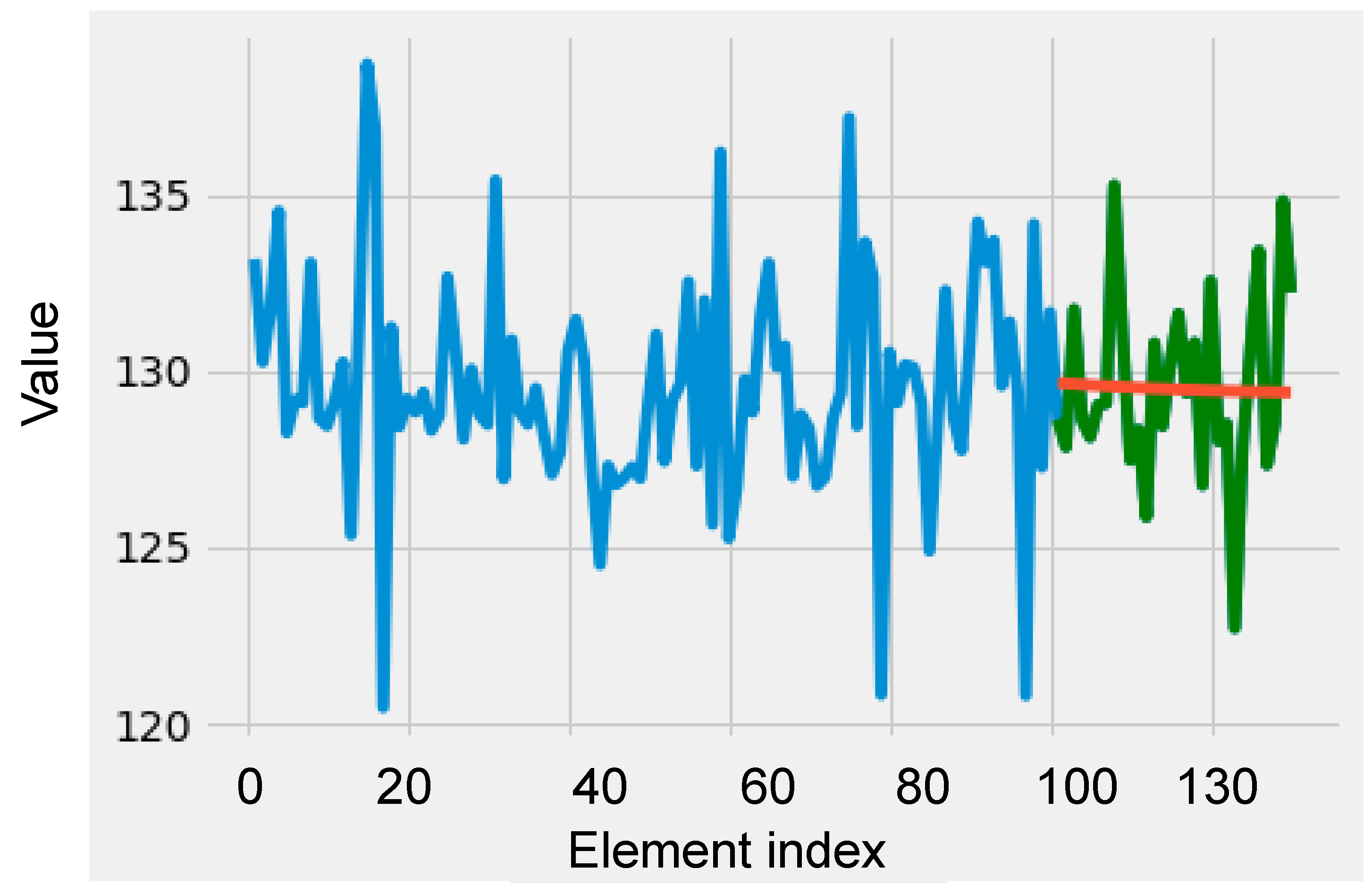
The predicted sequence can be seen in Figure 15. The developed model uses the initial sequence (blue color) of 100 values to obtain the prediction (red color). The prediction is then compared with the expected values (green color).

The sequence of expected values and the values obtained through the mean square error are compared to evaluate the model. These sequences can be seen in Figure 14.

The mean squared error (MSE), (4) is defined by the mean of the squared difference of the expected $\left(y_i\right)$ values and the obtained $\left(x_i\right)$ values divided by the number of sequence elements:

$$MSE=\frac{1}{n}\sum _{i=1}^n{(y_i-x_i)}^2.$$

(4)

The result obtained by calculating the MSE is positive, and the closer to 0, the better the model performance. After calculating the MSE, the result obtained for the model evaluation metric was 8.3783. This value normalized between zero and one was 0.0002, a value that reflected a good model prediction.

8. Data Collection Form

After the technical validation of the model, another means of validation of the developed prototype was performed. For this purpose, a form of questions regarding the prototype was prepared and directed to a group of specialists in analytics at Continental Advanced Antenna. Obtaining answers to the questionnaire from the mentioned experts allowed an evaluation of the developed prototype to draw conclusions about its validity concerning three different perspectives: effectiveness, efficiency, and satisfaction.

The methodology used in the prototype validation was inspired by the focus group research method, which suggests obtaining data by interacting (through questions) with a group of people. As such, the methodology considered the following steps:

• Selection of the group of people: The questionnaire was addressed to seven expert members of the analytics department of Continental Advanced Antenna, as mentioned. This group of experts was selected since they had qualifications that allowed us to obtain valid answers and they were properly accustomed to the environment under which the prototype was produced.
• Identification of the aspects under evaluation: The questionnaire focused on framing questions in three different aspects, namely effectiveness, efficiency, and satisfaction. The effectiveness of the prototype checked whether it was accurate for achieving specific objectives. On the other hand, efficiency aimed to assess the performance of the entity responsible for developing the prototype concerning the degree of difficulty associated with the tasks performed. Finally, satisfaction allowed us to evaluate the perception of the interviewee about the prototype developed.
• Data collection method: A questionnaire was developed to collect data on the aspects under evaluation identified in the previous item. This questionnaire included 12 questions related to the developed prototype, and each question had five response options. The answer range comprised a static list (1—strongly disagree; 2—disagree; 3—neither agree nor disagree; 4—agree; 5—strongly agree).
• Data collection procedure: Initially, seven expert members of the Continental Advanced Antenna were gathered and, after proper contextualization and explanation of the prototype, were asked, individually, the 12 questions duly grouped into the aspects under evaluation.

The questions that made up the developed questionnaire are listed below:

1

Do you understand what the application does?

2

Does the user interface have a friendly and perceptible layout?

3

Does the application allow the user to monitor trends?

4

Do you consider the obtained forecast of values easy to understand?

5

Is the developed application unnecessarily complex?

6

Are the tasks performed by the system well-integrated?

7

Do you consider the information obtained through warnings perceptible?

8

Do you think it would be necessary to obtain the aid of an expert to help you use this system?

9

Do you consider that the monitoring of the values can help to prevent anomalies in the EOL?

10

Do you consider that the forecasting of values can help to prevent anomalies in the EOL?

11

Do you think the application still needs to be worked on?

12

Are you satisfied with how the system performs?

Table 1. Answers obtained from the validation form.

	Collaborator ID
Question N°	ID 1	ID 2	ID 3	ID 4	ID 5	ID 6	ID 7
1	2	4	5	4	5	4	4
2	1	4	3	4	4	4	3
3	4	3	3	2	4	5	5
4	3	4	3	3	5	4	5
5	3	2	2	2	2	2	2
6	3	4	2	4	4	4	4
7	2	5	4	3	4	5	5
8	4	3	4	3	3	4	4
9	4	4	4	4	4	4	4
10	4	4	3	3	4	4	5
11	5	4	4	2	4	3	3
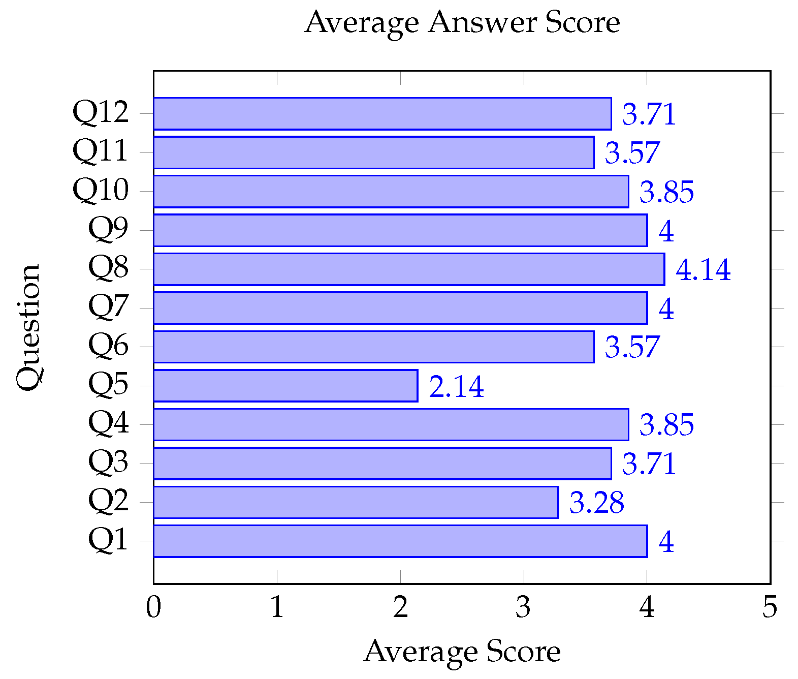
12	2	4	3	4	4	4	5

presents the feedback from the form directed at the collaborators. This prototype validation method allowed us to obtain various responses from different participants.

Figure 16 represents the average values obtained for each of the 12 questions asked to the experts. The average result is rounded.

In conclusion, this prototype validation method allowed us to obtain various answers from different participants. Overall, and based on the intended goals, the results were promising. Therefore, the developed prototype was considered by most experts as an added value for the end-of-line system, reflecting a range of advantages associated with detecting and preventing anomalies.

9. Discussion

Other models could have been used to simulate the same effect for the prediction, and the following discussion goes through some of these models exploiting their pros and cons in relationship to replacing the LSTM network. Although a random forest can handle nonlinear relationships in data and can handle mixed data types, it can also be slow for large datasets and may overfit without proper tuning. Although an SVM can handle nonlinear relationships in data and is effective for high-dimensional data, it is also slow for large datasets, sensitive to outliers, and requires a proper tuning of regularization parameters. Finally, a CNN is very effective for image and time-series data classification; however, in this particular case we do not seek a classification, but instead, we focus on obtaining a prediction. The choice of model ultimately depends on the specific problem and the characteristics of the data being analyzed, so we decided that for this particular case, the LSTM network was the most appropriate model.

The market implications of using machine learning algorithms such as the LSTM network in industrial manufacturing systems can be significant. By detecting and preventing anomalies in the production line, companies can increase the efficiency and reliability of their operations, leading to improved product quality, reduced production time, and increased competitiveness in the market. Predictive maintenance and resource scalability can also help organizations optimize their resources and reduce costs, making them more financially sustainable and competitive in the market.

From a practical perspective, the use of machine learning algorithms in industrial manufacturing systems can help organizations make better use of their data and improve decision-making. By automating the process of data analysis and anomaly detection, organizations can reduce the time and effort required to identify problems, allowing them to take prompt and effective corrective action.

The social implications of using machine learning algorithms in industrial manufacturing systems are also important. By improving the reliability and efficiency of industrial operations, organizations can reduce waste, conserve resources, and improve working conditions for employees. In addition, by detecting and correcting anomalies in the production line, organizations can help to prevent accidents, reduce harm to the environment, and improve the overall quality of life in the community.

This approach may also be applied in larger contexts in several ways, for example, in supply chain management, to monitor and analyze data from various stages of the supply chain, from raw material procurement to product delivery, to detect anomalies and optimize the entire supply chain; for quality control, to analyze data from product testing and inspection, enabling organizations to detect defects and improve the quality of their products; for resource optimization, to optimize resource utilization, reduce waste, and improve operational efficiency. Another application could be in predictive demand forecasting to analyze historical sales data and predict future demand, enabling organizations to optimize production and distribution.

The process of applying these types of models to industrial manufacturing systems can help organizations make decisions at various levels, such as the operational level, the maintenance level, and the management level. The monitoring and analyzing of real-time data from production lines, detecting anomalies and triggering alarms in real time, may help operators make quick and effective decisions to correct problems and minimize disruptions to the production process. The forecast of equipment failures enables organizations to schedule maintenance activities proactively, reducing downtime and improving equipment reliability, which may also provide managers with insights into production performance, resource utilization, and product quality.

The use of these algorithms for anomaly detection in industrial manufacturing systems can thus impact decision making at all levels of an organization, from front-line operators to senior management. By automating the process of data analysis and anomaly detection, organizations can make better informed decisions, reduce the time and effort required to identify problems, and take prompt and effective corrective action.

10. Conclusions

This paper presented a prototype of a system capable of predicting and anticipating trends in the testing system of antennas manufactured at Continental Advanced Antenna. Furthermore, to complement the information acquired for the work development, the topic of artificial intelligence, specifically machine learning, was addressed. The main focus was the study of the testing system, starting from the text files made available with the objective of analyzing the behavior of the testing system. The goal was achieved based on this objective and a methodology focused on obtaining results in specific tasks. The presented prototype allowed the interpretation of the progression of the antenna testing values in the production line through a data analysis, where afterward, it was also possible to obtain a prediction concerning the sequence of the next antennas to be produced. This innovation was an added value for the testing line in question since it allowed its monitoring and management based on the progression of the results under test.

In future work, it is suggested to integrate the LSTM network into the user interface developed to complement the analysis of the data exposed in the graph working as a service. It is also intended to implement the prototype in a layer of the industrial Internet of things’ ecosystem in which data are directly sent to the system and constantly processed, as specified by the application design. When a trend emerges, the system can anticipate it, offering advantages to the factory. New functionalities could also be added to the developed prototype, such as a sound system when the onset of a trend is evident, to increase the reach of alerts to the operators.