Graph-Augmentation-Free Self-Supervised Learning for Social Recommendation

Abstract

Social recommendation systems can improve recommendation quality in cases of sparse user–item interaction data, which has attracted the industry’s attention. In reality, social recommendation systems mostly mine real user preferences from social networks. However, trust relationships in social networks are complex and it is difficult to extract valuable user preference information, which worsens recommendation performance. To address this problem, this paper proposes a social recommendation algorithm based on multi-graph contrastive learning. To ensure the reliability of user preferences, the algorithm builds multiple enhanced user relationship views of the user’s social network and encodes multi-view high-order relationship learning node representations using graph and hypergraph convolutional networks. Considering the effect of the long-tail phenomenon, graph-augmentation-free self-supervised learning is used as an auxiliary task to contrastively enhance node representations by adding uniform noise to each layer of encoder embeddings. Three open datasets were used to evaluate the algorithm, and it was compared to well-known recommendation systems. The experimental studies demonstrated the superiority of the algorithm.

1. Introduction

With the advancement of the Internet, social platforms, such as WeChat, Weibo, and Twitter, have become an essential part of people’s daily lives. More and more users like to express their opinions and present their hobbies on these platforms, and the interactions between users result in a wide range of consumption behaviors. Moreover, social homogeneity [1] and social influence theory [2] demonstrate that connected users in social networks have similar interest preferences and continue to influence one another as information spreads. Based on these findings, social relations are frequently integrated into recommender systems as a powerful supplement to user–item interaction information to address the problem of data sparsity [3], and numerous social recommendation methods have been developed. Social recommendation algorithms based on graph neural networks have demonstrated improved performance recently and helped advance recommendation technology; however, these models still have certain drawbacks.

1. Interaction data are sparse and noisy. Most recommendation models utilize supervised learning techniques [4,5], which substantially rely on user–item interaction data and are unable to develop high-quality user–item representations when data are sparse. As a result, cold-start problems usually occur. In addition, GNN-based recommendation algorithms must aggregate and propagate node embeddings and their neighbors during training, which amplifies the impact of interaction noise (i.e., user mis-click behavior), resulting in confusion with regard to user preferences.

2. The effect of the long-tail phenomenon. Due to the skewed distribution of interactive data [4], the recommendation algorithm only emphasizes a portion of some users’ mainstream interests, resulting in underfitting of the sample tail distribution and trapping of the user’s interest in the “filter bubble” [6], which is known as the long-tail phenomenon.

3. Noise in social relationships. Existing recommendation models are generally based on the assumption that users in social networks have similar item preferences. However, the formation of social relationships is a complicated process that can be based on interests or pure social relationships. Users may have completely different preferences for certain items, but this is not always the case. The model becomes noisier as a result of this assumption, which makes it difficult to effectively incorporate user characteristics and recommendation targets in social networks.

Present work. In view of the above limitations and challenges, this paper proposes an improved social recommendation model—graph-augmentation-free self-supervised learning for social recommendation (GAFSRec). Here, we applied self-supervised contrastive learning to recommendation with the goal of increasing the mutual information for the same user/item view, thereby reducing the reliance on labels and resolving the first and second issues mentioned above. Most contrastive learning techniques currently in use (such as random edge/node loss) improve the consistency of nodes across views through structural perturbations [4,7,8,9]. However, the most recent research demonstrates [10] that data augmentation can still be accomplished without structural perturbation by adding the proper amount of random uniform noise to the original image. As a result, we employed the method of adding sufficiently small and uniform noise to the graph convolution layer of the recommendation task to achieve cross-layer comparative learning. This technique can operate in the embedding space, making it more effective and simpler to use, and it can subtly attenuate the long-tail phenomenon. The third problem was solved by using both explicit and implicit social relationships, employing hypergraph convolutional networks to mine users’ high-order social relationships, and adding the role of key opinion leaders to prevent extra social noise from affecting user preferences.

To improve efficiency, we employed a multi-task training technique with recommendation as the primary task and self-supervised contrastive learning as an auxiliary task. We first created four views using a social network graph and a user–item interaction graph: user–item interaction graph, explicit friend social graph, implicit friend social graph, and user–item sharing graph with explicit friends. Graph encoders (a graph convolutional network and hypergraph convolutional network) were then built for each view to learn the users’ high-order relational representation. To avoid the difficulties caused by data sparsity in modeling, we incorporated cross-layer contrastive learning without graph augmentation into GAFSRec, amplified the variance via a graph convolutional neural network, and regularized the representation of recommendations with contrast-augmented views. Finally, we combined the recommendation task and the self-supervised task within the framework of master-assisted learning. The performance of the recommendation task was significantly improved after jointly optimizing these two tasks and utilizing the interactions between all components.

The main contributions of this paper can be summarized as follows:

• We designed a high-order heterogeneous graph based on motifs, integrated social relations and item ratings, comprehensively modeled relational information in the network, and undertook modeling through graph convolution to capture high-order relations between users;
• We incorporated the cross-layer self-supervised contrastive learning task without graph augmentation into network training, enabling it to run more efficiently while ensuring the reliability of recommendations;
• We conducted extensive experiments with multiple real datasets, and the comparative results showed that the proposed model was superior and that the model was effective in ablation experiments.

The rest of this paper is organized as follows. Section 2 presents related work. Section 3 describes the framework for the multi-graph contrastive social recommendation model. Section 4 presents the experimental results and analysis. Finally, Section 5 brings the paper to a close.

2. Related Work

2.1. Graph-Based Recommendation

To obtain high-order collaborative signals, graph-based recommendation algorithms employ multi-hop interaction topologies [11,12]. The success of graph convolutional neural network technology served as inspiration for Feng et al. [10] to develop a hypergraph representation learning framework that captures the relationship between high-order data by developing hyperedge convolution operations. Hypergraphs have a flexible topology and can be used to model complex and high-order dependencies. Additionally, some recently created recommender systems, such as HyperRec [13], MHCN [9], and HCCF [14], have begun to use hypergraph topologies to capture high-order interactions among nodes. HyperRec [13] applies numerous convolutional layers to hypergraphs to capture multi-level connections in order to describe short-term item correlation features. In order to mine high-order user relationship patterns, Yu et al. [9] presented a multi-channel hypergraph convolutional network (MHCN) and created numerous topic-induced hypergraphs. They also employed self-supervised learning to boost the learning of mutual information shared between channels. The application of hypergraphs to social recommendations is made possible by the retention of more high-level information. By simultaneously collecting local and global cooperation information through a hypergraph-enhanced cross-view contrastive learning architecture, HCCF [14] overcomes the over-smoothing problem. In comparison, our system makes use of hypergraph encoders to help create heterogeneous networks, maintain the collaborative relationship between users and items, and enhance the ability to identify user preferences.

2.2. Self-Supervised Contrastive Learning

Self-supervised learning is divided into two categories: generative models and contrastive models. The goal of creating a model is to reconstruct the input so that the input and output are as similar as possible using techniques such as GAN [15] and VAE [16] autoencoders. Contrastive models have recently emerged as an effective self-supervised framework for capturing feature representation consistency across different viewpoints.

Model contrasts are classified into three types [17]: structure-level contrasts, feature-level contrasts, and model-level contrasts. Local–local and global–global structural-level comparison targets exist. SGL [8] is a typical representative, changing the structure of graphs through local perturbations (node loss, edge loss, and random walk). These data enhancement and pre-training methods can extract more supervisory signals from the original graph data, allowing the graph neural network to learn node representation more effectively. Due to dataset constraints, feature-level comparisons have received less attention. Model-level comparison can be implemented end-to-end relatively easily, and SimGCL [10] directly adds noise to the embedding space for enhancement. Experiments show that, regardless of whether graph enhancement is used or not, optimization of the contrast loss can help learn representations. To model node embeddings, we used a cross-layer contrastive learning method without graph augmentation in this study.

3. Proposed Model

3.1. Preliminaries

Let $U=\{u_1,u_2,\cdots ,u_m\}(\left|U\right|=m)$ represent the collection of users and $I=\{i_1,i_2,\cdots ,i_n\}(\left|I\right|=n)$ represent the collection of items. Since we are focused on item recommendation, we define $\mathit{R}\in {ℝ}^{m\times n}$ to represent the user–item interaction binary matrix. For each pair $(u,i)$, $r_{ui}=1$ indicates that user $u$ has interacted with item $i$ and, conversely, $r_{ui}=0$ indicates that user $u$ has not interacted with item $i$ or that user $u$ is not interested in item $i$. We represent social relations using directed social networks, where $\mathit{S}\in {ℝ}^{m\times m}$ represents an asymmetric relation matrix. Additionally, $\{{\mathit{Z}}_u^{(1)},{\mathit{Z}}_u^{(2)},\cdots ,{\mathit{Z}}_u^{(l)}\}\in {ℝ}^{m\times d}$ and $\{{\mathit{Z}}_i^{(1)},{\mathit{Z}}_i^{(2)},\cdots ,{\mathit{Z}}_i^{(l)}\}\in {ℝ}^{n\times d}$ denote the embeddings of the size d-dimensional users and items learned in each layer, respectively. This article uses bold uppercase letters for matrices and bold lowercase letters for vectors.

Definition 1.

Hypergraph.

Let $G=(V,E)$ represent a hypergraph, V a vertex set containing N vertices in the hypergraph, and E an edge set containing M hyperedges. Each hyperedge $\epsilon \in E$ contains two or more vertices and is assigned a positive weight $W_{\epsilon \epsilon }$. All weights form a diagonal matrix $W\in {ℝ}^{M\times M}$. A hypergraph is represented by an incidence matrix $H\in {ℝ}^{N\times M}$, which is defined as follows:

$$H_{i,j}=\{\begin{array}{l}1,\mathrm{if}{v}_i\in V\\ 0,\mathrm{if}{v}_i\notin V\end{array}$$

(1)

If the hyperedge ${\epsilon }_j\in E$ contains a vertex, then $H_{i,j}=1$; otherwise, $H_{i,j}=0$. The degrees of the vertices and edges of a hypergraph are represented as follows: $D_v={\displaystyle {\sum }_{\epsilon =1}^M{W}_{\epsilon \epsilon }{H}_{i\epsilon }}$; $D_e={\displaystyle {\sum }_{i=1}^N{H}_{i\epsilon }}$.

3.2. High-Order Social Information Exploitation

In this study, we used two graphs as data sources: a user–item interaction graph $G_r$ and a user social network graph.

We aligned the two networks into a heterogeneous network and divided it into three sets of views—an explicit friend social graph, an implicit friend social graph, and items shared by users with explicit friends’ graphs—in order to establish high-order associations between users in the network. The project-sharing graph of users and explicit friends describes a user’s interest in sharing items with friends, which can also serve as relationship-strengthening. The social graph of explicit friends describes a user’s interest in expanding their social circle. The social graph of implicit friends describes the similar interests a user shares with similar but unfamiliar users and can alleviate the negative impact of unreliable social relations.

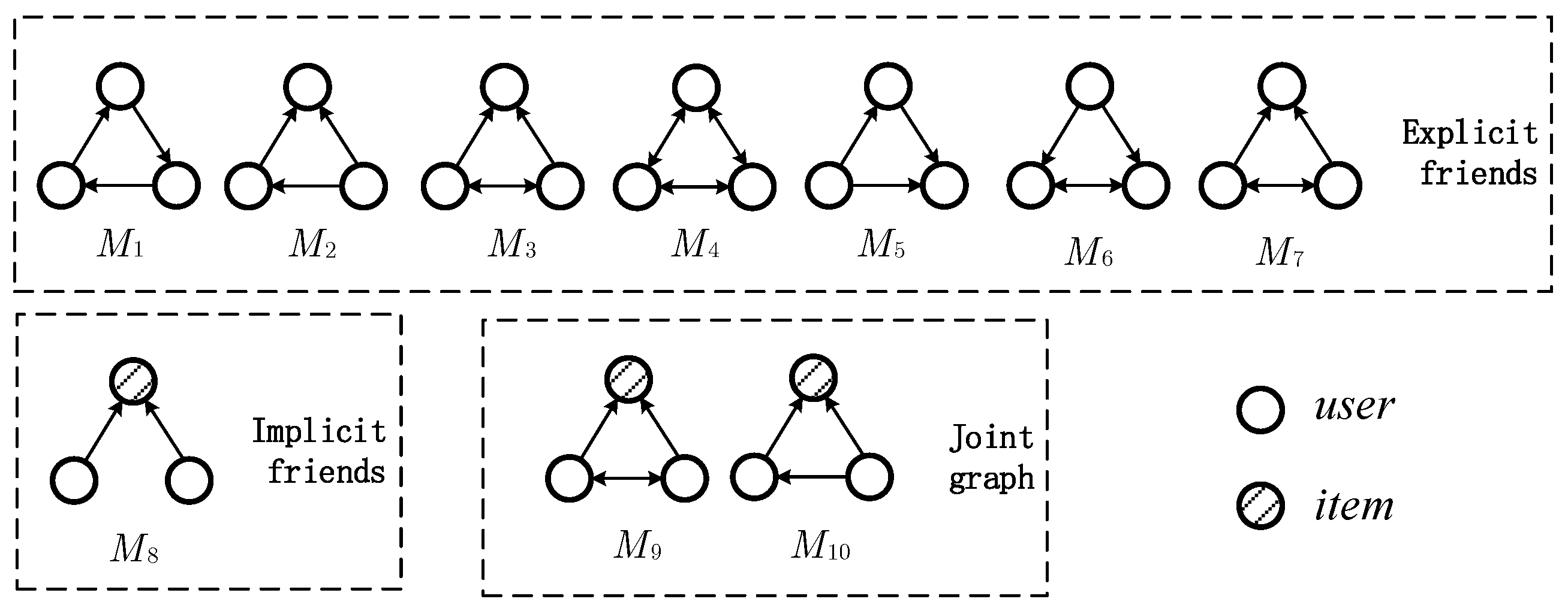
Taking into account the fact that there are some significant social network structures that have impacts on the authority and reputation of nodes in the representation of higher-order relationships as network motifs, we used the motif-based PageRank [18] framework. PageRank is a general algorithm for ranking users in social networks [19]. It can be utilized as a measurement standard for opinion-leader mining, impact, and credibility analyses by assessing the authority of network nodes. However, only edge-based relations are exploited, with higher-order structures in complex networks being neglected. This aspect is improved by the motif-based PageRank algorithm. As shown by Figure 1, which covers the fundamental and significant user social types, the user–item interaction graph splits the explicit friend social graph into seven motifs. M8, also defined as the user’s implicit friend social network, represents strangers who share the user’s interests. The relationship M9–M10, generally described as users’ and explicit friends’ item-sharing graph, is, at the same time, extended in accordance with friends’ shared buying behaviors.

When given any motif set $M_k$, we can calculate the adjacency matrix of the motif using

Table 1. Computation of motif-based adjacency matrices.

Motif	Matrix Computation	${\mathit{A}}_{{\mathit{M}}_{\mathit{i}}}$
$M_1$	$C=(U\cdot U)\odot U^T$	$C+C^T$
$M_2$	$C=(B\cdot U)\odot U^T+(U\cdot B)\odot U^T+(U\cdot U)\odot B$	$C+C^T$
$M_3$	$C=(B\cdot B)\odot U+(B\cdot U)\odot B+(U\cdot B)\odot B$	$C+C^T$
$M_4$	$C=(B\cdot B)\odot B$	$C$
$M_5$	$C=(U\cdot U)\odot U^T+(U\cdot U^T)\odot U+(U^T\cdot U)\odot U$	$C+C^T$
$M_6$	$C=(U\cdot B)\odot U+(B\cdot U)\odot U^T+(U^T\cdot U)\odot B$	$C$
$M_7$	$C=(U^T\cdot B)\odot U^T+(B\cdot U)\odot U+(U\cdot U^T)\odot B$	$C$
$M_8$	$C=R\cdot R^T$	$C$
$M_9$	$C=(R\cdot R^T)\odot B$	$C$
$M_{10}$	$C=(R\cdot R^T)\odot U$	$C+C^T$

.

$${(A_M)}_{i,j}={\displaystyle \sum _{i\in U,j\in U}1(i,joccurin{M}_k)}$$

(2)

In Table 1, $B=S\odot S^T$ and $U=S-B$ are the adjacency matrices of two-way and one-way social networks respectively. Without considering self-connections, $A_e={\displaystyle {\sum }_{k=1}^7{A}_{M_K}}$, $A_i=A_{M_8}$, and $A_j=A_{M_9}+A_{M_{10}}$, where, in $A_j=A_{M_9}+A_{M_{10}}$, we only keep values greater than 5 for the reliability of the implicit friend pair experiment. Furthermore, the adjacency matrix for the user–items graph is ${\mathit{A}}_r=\mathit{R}$.

3.3. Graph Collaborative Filtering BackBone

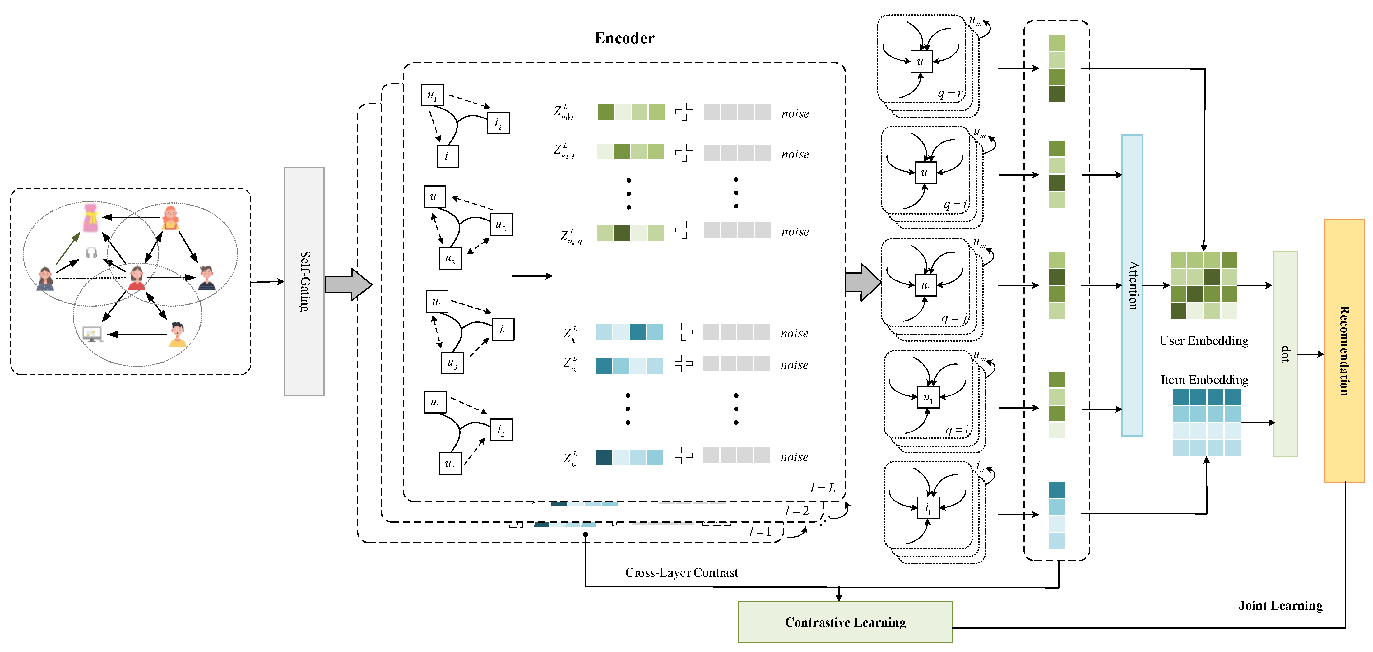
In this section, we present our model GAFSRec. In Figure 2, the schematic overview of our model is illustrated.

Due to its strong ability to capture node dependencies, we adopted LightGCN [20] to aggregate neighborhood information. Formally, a general GCN is constructed using the following hierarchical propagation:

$${\mathit{Z}}^{(l)}={\mathit{D}}^{-1}\mathit{A}{\mathit{Z}}^{(l-1)}$$

(3)

where $Z^{(l)}$ is the l-th layer embedding of the node, and $G_q\in \{G_r,G_e,G_i,G_j\}$ are the four views, with A being the adjacency matrix and D the degree diagonal matrix of A. We encoded the original node vectors into the embedding vectors required by each view through gating functions.

$${\mathit{Z}}_{q\in \{r,e,i,j\}}^{(0)}={\mathit{Z}}^{(0)}\odot \sigma ({\mathit{Z}}^{(0)}{\mathit{W}}_g^q+{\mathit{b}}_g^q)$$

(4)

where $\sigma$, ${\mathit{W}}_g^q\in {ℝ}^{d\times d}$, and ${\mathit{b}}_g^q\in {ℝ}^d$ are the activation function, weight matrix, and bias vector. $q\in \{r,e,i,j\}$ represents four views. ${\mathit{Z}}^{(0)}$ denotes the initial embedding vector and $\odot$ represents the dot product.

We used the generalization ability of hypergraph modeling to capture more effective high-level user information. Therefore, in the encoder, a hypergraph convolutional neural network [21] was used.

$${\mathit{Z}}^{(l)}={\mathit{D}}^{-1}\mathit{A}{\mathit{Z}}^{(l-1)}={\mathit{D}}_v^{-1}\mathit{H}\mathit{W}{\mathit{D}}_e^{-1}{\mathit{H}}^T{\mathit{Z}}^{(l-1)}$$

(5)

where $\mathit{A}=\mathit{H}\mathit{W}{\mathit{D}}_e^{-1}{\mathit{H}}^T$ is the Laplacian matrix of the hypergraph convolutional network; H is the incidence matrix of each hypergraph; ${\mathit{D}}_v$ and ${\mathit{D}}_e$ are the degree matrix of the nodes and the degree matrix of the hyperedges; and $\sigma$, $\mathsf{\Theta }$, and $\mathit{W}$ are activation functions, learnable filter matrices, and the parameters of the diagonal matrix.

Considering node influence and credibility, we adopted motifs [18] to construct a hypergraph. Given the complexity of the actual construction of the Laplacian matrix for hypergraph convolution (which includes a large number of graph-induced hyperedges), matrix multiplication can be considered for simplification.

Finally, the hypergraph convolutional neural network can be expressed as: ${\mathit{Z}}_{q\in \{r,e,i,j\}}^{(l)}={\tilde{\mathit{D}}}_q^{-1}{\mathit{A}}_q{\mathit{Z}}_q^{(l-1)}$, where ${\tilde{\mathit{D}}}_q\in {ℝ}^{m\times m}$ is the degree matrix of ${\mathit{A}}_q$. It can be seen from this that the graph convolutional neural network is a special case of the hypergraph neural network.

After l-layer propagation, we used the weighting functions and the readout function to output the representations of all layers, obtaining the following representations:

$${\mathit{Z}}_{u|q}=\frac{1}{L+1}{\displaystyle \sum _{l=0}^L{\mathit{Z}}_{u|q}^{(l)}},{\mathit{Z}}_{i|q}=\frac{1}{L+1}{\displaystyle \sum _{l=0}^L{\mathit{Z}}_{i|q}^{(l)}}$$

We applied an attention approach [22] to learn the weights α and aggregate the user embedding vectors for augmented views.

$${\alpha }_q=\frac{\exp ({\mathit{a}}^T{\mathit{W}}_a{\mathit{Z}}_{u|q})}{{\displaystyle \sum _{q^{\prime }\in \{e,i,j\}}\exp ({\mathit{a}}^T{\mathit{W}}_a{\mathit{Z}}_{u|q^{\prime }})}}$$

where $a$ and $\mathit{W}$ are trainable parameters. The final user embedding ${\mathit{Z}}_u$ and item embedding ${\mathit{Z}}_i$ look like this:

$$\begin{array}{l}{\mathit{Z}}_u={\displaystyle {\sum }_{q\in \{e,i,j\}}}{\alpha }_q{\mathit{Z}}_{u|q}+{\displaystyle \sum _{l=0}^L{\mathit{Z}}_{u|r}^{(l)}}\\ {\mathit{Z}}_i=\frac{1}{L+1}{\displaystyle \sum _{l=0}^L{\mathit{Z}}_{i|r}^{(l)}}\end{array}$$

The ranking score generated by this model recommendation is defined as the inner product with user and item embeddings:

$${\stackrel{⌢}{y}}_{u,i}={\mathit{Z}}_u^T{\mathit{Z}}_i$$

To optimize the parameters in the model, we adopted the Bayesian loss function [23]. The main reason was that the Bayesian loss function considers the comparison of pairwise preferences between observed interactions and unobserved interactions. The loss function of this model is:

$${ℒ}_{BPR}=-{\displaystyle \sum _{i\in I(u),j\notin I(u)}}\ln \sigma ({\stackrel{⌢}{y}}_{u,i}-{\stackrel{⌢}{y}}_{u,j})+\beta {\Vert \mathsf{\Phi }\Vert }_2^2$$

where $\mathsf{\Phi }$ is a trainable parameter and $\beta$ is a regularization coefficient that controls the strength of L2 regularization, prevents overfitting, and is a sigmoid function. Each input datum is a triplet sample < u, i, j >; this triplet includes the current user u, the positive item i purchased by u, and the randomly drawn negative item j. The negative item j is the user u’s unliked or unknown items.

3.4. Graph-Augmentation-Free Self-Supervised Learning

Data augmentation is the premise of self-supervised contrastive learning models, and they can obtain a more uniform representation by perturbing the structure and optimizing the contrastive loss. With regard to the learning of graph representations, a study on SimGCL [10] showed that it is the uniformity of distribution rather than dropout-based graph augmentation that has the greatest impact on the performance of self-supervised graph learning. Therefore, we considered adding random noise to the embedding to create a self-supervised signal that could enhance the performance of the contrastive learning.

$${\tilde{\mathit{Z}}}^{(l)}={\mathit{D}}^{-1}\mathit{A}{\tilde{\mathit{Z}}}^{(l-1)}+{\epsilon }^{(l)}$$

where ε is the added random uniform noise vector, and the noise direction is in the same direction as the embedding vector, $\epsilon =x\odot sign(z)$, $x\in {ℝ}^d~U(0,1)$. The embedding representation added with perturbation retains most of the information of the original representation, as well as some invariance.

By applying different scales of embedding vectors to the current node embedding, the perturbed embedding vectors can then be fed into the encoder. The embedding vector of the final perturbed node is expressed as:

$$\tilde{\mathit{Z}}=\frac{1}{L+1}{\displaystyle \sum _{l=0}^L{\tilde{\mathit{Z}}}^{(l)}}$$

We regarded augmented views from the same node as positive examples and augmented views from different nodes as negative examples. Positive auxiliary supervision promotes the consistency of predictions among different views of the same node, while negative supervision strengthens the divergence between different nodes. Formally, we adopted the contrastive loss InfoNCE [24] to maximize the consistency of positive examples and minimize the consistency of negative examples:

$${ℒ}_{cl}^U=-{\displaystyle \sum _{u\in \mathcal{U}}\log \frac{\exp (sim({\tilde{z}}_u^{(k)}\cdot {\tilde{z}}_u)/\tau )}{{\displaystyle {\sum }_{v\in \mathcal{U}}\exp (sim({\tilde{z}}_u^{(k)}\cdot {\tilde{z}}_v)/\tau )}}},{ℒ}_{cl}^I=-{\displaystyle \sum _{i\in ℐ}\log \frac{\exp (sim({\tilde{z}}_i^{(k)}\cdot {\tilde{z}}_i)/\tau )}{{\displaystyle {\sum }_{j\in ℐ}\exp (sim({\tilde{z}}_i^{(k)}\cdot {\tilde{z}}_j)/\tau )}}}$$

where ${\tilde{z}}_u^{(k)}={\tilde{z}}_u^{(k)}/{\Vert {\tilde{z}}_u^{(k)}\Vert }_2$ represents the k-th layer L2-regularized embedding vector compared with the final layer embedding, $sim\left(a,b\right)$ represents the dot-product cosine similarity between normalized embeddings, and b. τ is the temperature parameter. The total loss function for self-supervised learning includes the contrastive loss for each view user and the item contrastive loss, as shown in the following equation:

$${ℒ}_{\mathrm{ssl}}={\displaystyle \sum _{q\in \{r,e.i,j\}}{ℒ}_{cl}^{q,U}}+{ℒ}_{cl}^{r,I}$$

To improve recommendation through contrastive learning, we utilized a multi-task training strategy to jointly optimize the recommendation task and the self-supervised learning task, as shown in the following equation:

$$ℒ={ℒ}_{BPR}+\lambda {ℒ}_{ssl}$$

where λ is the hyperparameter used to control the auxiliary task.

3.5. Complexity Analysis

In this section, we analyze the theoretical complexity of GAFSRec. Since the time complexity of LightGCN-based convolutional graph encoding is $O(L\times \left|\mathit{R}\right|\times d)$, the total encoder complexity of this architecture is less than $4\times O(L\times \left|\mathit{R}\right|\times d)$ because the adjacency matrix of the auxiliary encoder is sparser than that of the user–item interaction graph. The time costs of the gate function and the aggregation layer are both $O(m\times d^2)$. This architecture adopts BPR loss; each batch contains B interactions, and the time cost is $O(2\times B\times d)$. 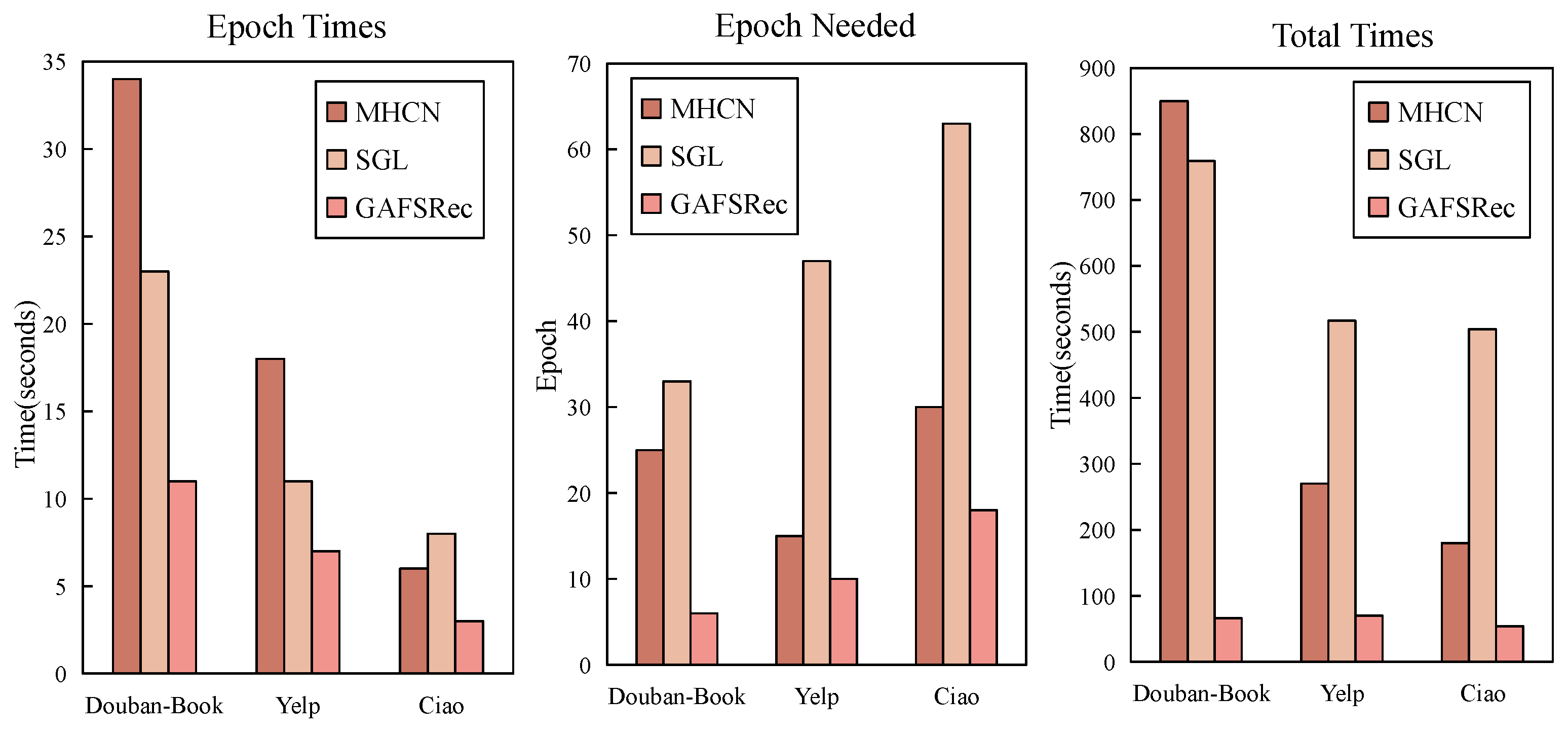Since the contrasting between positive/negative samples in contrastive learning increases the time cost, cross-layer self-supervised contrastive learning contributes a time complexity of $5\times O(B\times M\times d)$, where M represents the number of nodes in a batch. Since this model does not involve graph augmentation, the complexity of GAFSRec is much lower than that of graph-augmented social recommendation models. In our experiments, with the same embedding size and using the Douban-Book dataset, MHCN took 34 s per epoch and GAFSRec only took 11 s. Detailed information on the experiments can be found in Section 4.2.1.

4. Experiments and Results

In this section, we describe the extensive experiments we conducted to validate GAFSRec. The experiments were conducted in order to answer the following three questions: (1) Does GAFSRec outperform state-of-the-art baselines? (2) Does each component in GAFSRec play a role? (3) What are the effects of hyperparameters on the GAFSRec model?

4.1. Experimental Settings

4.1.1. Datasets

We conducted experiments using three real-world datasets: Douban-Book [25], Yelp [26], and Ciao [5]. The statistical data for the datasets are shown in

Table 2. Data statistics for social recommendation datasets.

	Douban-Book	Yelp	Ciao
Users (U-I graph)	12,859	19,539	7375
Users (U-U graph)	12,748	30,934	7317
Items	22,294	22,228	105,114
Feedback	598,420	450,884	284,086
Valid user pairs	48,542,437	51,061,951	5,052,316
Social pairs	169,150	864,157	111,781
Valid social pairs	77,508	368,405	56,267
Candidate user pairs	165,353,881	381,772,521	54,390,625
Valid ratio	29.357%	13.375%	9.289%
Valid social ratio	45.822%	42.632%	50.337%
Social density	0.104%	0.090%	0.209%
Rating density	0.209%	0.104%	0.037%
Social diffusity level	1.561	3.187	5.419
Valid social density	0.160%	0.721%	1.114%

. In accordance with the summary provided by Tao et al. [27], we conducted statistical analyses of the three datasets, which were helpful for the analysis of the results of the subsequent experiments. It was found that the higher the level of social diffusion was (greater than 1), the greater the possibility of similar preferences among users was, and the higher the effective social density was, the lower the scoring density was, indicating that explicit social relationships are very important for recommendation. We performed fivefold cross-validation with the three datasets and report the averaged results.

4.1.2. Baselines

We evaluated GAFSRec against 13 baselines spanning different recommendations:

• MF-based collaborative filtering models;
• BPR [23]: a popular recommendation model based on Bayesian personalized ranking;
• SBPR [28]: an MF-based social recommendation model that extends BPR and utilizes social relations to model the relative order of candidate items;
• GNN-based collaborative filtering frameworks;
• NGCF [7]: a complex GCN-based recommendation model that generates user/item representations by aggregating feature embeddings with high-order connection information;
• LightGCN [20]: a general recommendation model based on GCN, improved on the basis of NGCF by removing linear changes and activation functions;
• DiffNET++ [29]: a GNN-based social recommendation method that simultaneously simulates the recursive dynamic social diffusion of user space and item space;
• Recommendation with hypergraph neural networks;
• MHCN [9]: a social recommendation method based on a motif-based hypergraph. It aggregates high-level user information through hypergraph convolutional multi-channel embedding and utilizes auxiliary tasks to maximize the mutual information between nodes and graphs and generate self-supervised signals;
• HyperRec [13]: this method leverages the hypergraph structure to model the relationship between users and their interactive items by considering multi-order information in dynamic environments;
• HCCF [14]: a hypergraph-guided self-supervised learning recommendation model that jointly captures local and global collaborations through a hypergraph-enhanced cross-view contrastive learning architecture;
• Self-supervised learning for recommendation;
• SEPT [25]: a social recommendation model that utilizes multiple views to generate supervisory signals;
• SGL [8]: the most typical self-supervised comparative learning recommendation model, which uses structural perturbation to generate comparative views and maximizes the consistency between nodes. The experiment in this study used the structural perturbation method involving missing edges;
• BUIR [30]: this method adopts two encoders that learn from each other and randomly generates augmented views for supervised training;
• SimGCL [10]: the latest self-supervised contrastive learning recommendation model. It uses the no-image-enhancement method and only adds the final embedding obtained by adding uniform noise in the embedding space for comparison;
• NCL [31]: a prototypal structural contrastive learning recommendation model.

4.1.3. Metrics

To evaluate all the models, we chose two evaluation metrics: Recall@K and NDCG@K. Recall@K employs the proportions of each user’s favorite items appearing in the recommended items. Normalized discounted cumulative gain (NDCG) means that the scores for the relevance of each recommendation result are accumulated and used as the score for the entire recommendation list. The greater the relevance of the recommendation result is, the greater the DCG is. The recall rate is defined as: $\mathrm{Recall}@\mathrm{K}=\frac{{\displaystyle {\sum }_{i=1}^{K}re{l}_i}}{\min (K,\left|{\mathrm{y}}_u^{test}\right|)}$. The normalized discounted cumulative gain is defined as $\mathrm{DCG}@\mathrm{K}={\displaystyle {\sum }_{i=1}^K\frac{2^{re{l}_i}-1}{{\log }_2(i+1)}}$ $\mathrm{NDCG}@\mathrm{K}=\frac{DCG@K}{iDCG@K}$.

4.1.4. Settings

To ensure a fair comparison, we checked the best hyperparameter settings reported in the original papers for the baselines and then used grid search to fine-tune all the hyperparameters for the baselines. For the general setup of all baselines, all embeddings were initialized with Xavier. The embedding size was 64, the L2 regularization parameter was β = 0.01, and the batch size was 2048. We optimized all models using Adam with a learning rate of 0.001 and let the temperature τ = 0.2.

4.2. Recommendation Performance

Next, we verified whether GAFSRec could outperform the baselines and achieve the expected performance. The purpose of social recommendation is to alleviate data sparsity. We also conducted a cold-start experiment with the entire training set. The cold-start experiment dataset only included the data for cold-start users with fewer than ten historical purchase records. The results are shown in

Table 3. General recommendation performance comparison.

Dataset	Metric	BPR	SBPR	NGCF	LightGCN	DiffNET++	HyperRec	MHCN	HCCF	BUIR	SLRec	SGL	SimGCL	NCL	GAFSRec	Improvement
Douban-Book	Recall@20	0.0889	0.0918	0.1167	0.0936	0.0988	0.1394	0.1487	0.1666	0.0982	0.1400	0.1617	0.1629	0.1650	0.1781	6.90%
	NDCG@20	0.0682	0.0717	0.0943	0.0770	0.0791	0.1260	0.1329	0.1421	0.0793	0.1263	0.1412	0.1422	0.1416	0.1637	15.17%
Yelp	Recall@20	0.0554	0.0665	0.0891	0.0820	0.0852	0.1120	0.1174	0.1157	0.0834	0.1126	0.1146	0.1145	0.1148	0.1292	12.37%
	NDCG@20	0.0289	0.0403	0.0533	0.0472	0.0496	0.0690	0.0746	0.0750	0.0482	0.0696	0.0732	0.0729	0.0741	0.0826	10.26%
Ciao	Recall@20	0.0412	0.0312	0.0517	0.0555	0.0477	0.0591	0.0629	0.0647	0.0528	0.0602	0.0635	0.0642	0.0625	0.0692	7.07%
	NDCG@20	0.0310	0.0252	0.0379	0.0426	0.0352	0.0400	0.0483	0.0502	0.0419	0.0468	0.0492	0.0501	0.0494	0.0522	3.88%

and

Table 4. Cold-start recommendation performance comparison.

Dataset	Method	BPR	SBPR	NGCF	LightGCN	DiffNET++	MHCN	HCCF	SGL	SimGCL	NCL	GAFSRec	Improvement
Douban-Book	Recall@20	0.0754	0.1045	0.1135	0.1108	0.1105	0.1755	0.1877	0.1929	0.1924	0.1725	0.1972	2.79%
	NDCG@20	0.0388	0.0879	0.0644	0.0631	0.0590	0.1043	0.1098	0.1154	0.1164	0.1024	0.1233	5.94%
Yelp	Recall@20	0.0619	0.0696	0.0881	0.0881	0.0917	0.1258	0.1271	0.1322	0.1212	0.1150	0.1330	5.89%
	NDCG@20	0.0296	0.0427	0.0415	0.0402	0.0420	0.0610	0.0662	0.0709	0.0625	0.0571	0.0669	11.57%
Ciao	Recall@20	0.0416	0.0413	0.0576	0.0544	0.0519	0.0638	0.0638	0.0605	0.0627	0.0635	0.0731	14.51%
	NDCG@20	0.0209	0.0251	0.0330	0.0324	0.0308	0.0340	0.0331	0.0338	0.0339	0.0338	0.0374	9.82%

. It can be observed that GAFSRec outperformed the baselines in general and cold-start cases with all datasets.

4.2.1. Comparison of Training Efficiency

In this section, we report the actual training time to verify the theoretical plausibility of the method. The reported data were collected using a workstation equipped with an Intel(R)Core™ i9-9900K CPU and a GeForce RTX 2080Ti GPU. The model depths of all methods were set to two layers.

As shown in Figure 3, compared with the MHCN and SGL models, GAFSRec demonstrated longer computation time due to the parallel processing of hierarchical self-supervised learning tasks in the MHCN model, and the running time also increased with the number of datasets. For SGL-ED, only the user–item interaction dataset was computed, and most of the runtime was spent on building the perturbation graph. In the large Douban-Book dataset especially, the speed of GAFSRec was three times faster than that of MHCN, thus demonstrating the strong advantage of graph-augmentation-free cross-layer contrastive learning in terms of operational efficiency.

4.2.2. Comparison of Ability to Promote Long-Tail Items

As mentioned in the introduction, GNN-based recommendation models are easily affected by the long-tail problem. To verify that GAFSRec could entirely alleviate the long-tail problem, we divided the test set into ten groups according to popularity. Each group contained the same numbers of interactions, and the larger the ID of a group was, the more popular the items were. Then, we set the number of layers to two for the experiments and verified the long-tail recommendation ability of the model by observing Recall@20.

As shown in Figure 4, LightGCN tended to recommend popular items and had the lowest recommendation ability for long-tail items (as illustrated in the small figure). Due to sparse interaction signals, it was difficult for LightGCN to obtain high-quality representations of long-tail items. However, with SimGCL, by optimizing the consistency of InfoNCE-loss learning representations, long-tail problems could be avoided as much as was possible, and excellent recommendation performance could be achieved. MHCN also optimized the InfoNCE loss through global and local comparisons but did not learn a more consistent representation, resulting in inferior performance to SimGCL when recommending long-tail items. In contrast, GAFSRec showed outstanding advantages when recommending long-tail products (such as GroupIDs 1, 2, and 3) and the highest recall value, but it was not as good as other models for GroupID 10. It can be seen that learning a more uniform representation by optimizing the InfoNCE loss can enable models to debias and alleviate the long-tail phenomenon, as well as increasing freshness and helping to meet user needs.

4.3. Ablation Study

4.3.1. Investigation of Multi-Graph Setting

To investigate the influence of high-order relationships in user social networks on recommendation, we first investigated the impact of individual views on recommendations by removing any one of the three social relationships’ views and leaving two remaining. As can be seen from Figure 5, removing any view resulted in performance degradation. The bars in the figure (except the complete bar) represent the cases with the corresponding views removed, while the complete bar represents the complete model.

Obviously, for the Douban-Book dataset, due to the low effective social density of the dataset, the explicit user view had little influence on the recommendation, while the recommendation performance of the view lacking the implicit user dropped sharply, indicating that the implicit user was the user. Items that met user needs were recommended, proving the key role of implicit users for recommendation. For the Yelp and Ciao datasets, due to the higher effective social density of the datasets, explicit user views had a greater impact on the recommendation. Figure 6 visualizes each graph’s attention score (median attention score for training set users), revealing that the implicit user had the highest attention score, while the explicit user and the joint graph had low attention scores. According to the findings shown in Figure 5 and Figure 6, implicit users contributed significantly to the analysis of user preferences while explicit users played a greater role when the social density was high, and the joint graph did not necessarily bring greater benefits due to social noise.

4.3.2. Investigation of Contrastive Learning Setting

In this study, we investigated the impact of contrastive learning on recommendation through two GCLSRec variants:

• Removing social recommendation for contrastive learning tasks (without CL);
• Disabling cross-layer comparison and using the final embedding of each layer embedding to add uniform noise and construct two sets of views for comparison of the learning task recommendations (CL-c).

The evaluation results are reported in

Table 5. Performance comparison of different GCLSRec variants.

Dataset	Douban-Book		Yelp		Ciao
Metric	Recall	NDCG	Recall	NDCG	Recall	NDCG
Top 20
Without CL	15.318%	13.371%	9.926%	6.175%	5.704%	4.265%
CL-c	17.716%	16.716%	12.870%	8.152%	6.644%	4.942%
CL-ours	17.806%	16.370%	12.922%	8.256%	6.922%	5.219%
Top 40
Without CL	15.958%	11.379%	14.123%	7.147%	8.633%	5.402%
CL-c	23.038%	18.055%	18.178%	9.815%	8.987%	5.737%
CL-ours	22.943%	17.724%	18.516%	10.045%	8.821%	5.628%

. It can be observed that not adding self-supervised contrastive learning (without CL) reduced the accuracy of recommendation, and when recommending top 40 items, the recommendation performance only improved slightly, as the aggregation mechanism of GCN can obscure high-order connection information. While model recommendation by constructing contrasting views individually (CL-ours) worked well, constructing contrasting views individually (CL-c) led to high model complexity and was time-consuming. However, GAFSRec with cross-layer comparative learning could not only guarantee recommendation accuracy but also had remarkably high recommendation efficiency.

4.4. Parameter Sensitivity Analysis

4.4.1. Influence of λ and ε

We observed the effect on the recommendation performance when the combination of λ and ε was changed. When λ was [0, 0.01, 0.05, 0.1, 0.2, 0.5, 1], ε was [0, 0.01, 0.05, 0.1, 0.2, 0.5, 1], and the number of model layers was set to two.

As shown in Figure 7, when fixing ε at 0.1, all parameters showed similar trend changes, and the best performance was achieved at specific λ values (Douban-Book dataset λ = 0.1, Yelp dataset λ = 0.05, Ciao dataset λ = 0.01). However, when λ was too large (λ = 0.5, 1), a significant performance drop could be seen.

We fixed λ at the best values for the three datasets, as reported in Figure 8, and then adjusted ε to observe the performance change. When ε = 0.01, the best recommendation performance (Douban-Book dataset and Yelp dataset) was achieved. However, when ε was too large or too small, the recommendation was especially vulnerable to changes in ε, so the performance declined faster. What can be seen from this is that GAFSRec was more sensitive to changes in λ, and with ε = 0.01, the model could maintain stable performance.

4.4.2. Layer Selection for Contrasting

For the recommendations using cross-layer contrastive learning, it is necessary to choose one of the embeddings of one layer and the final embedding for the comparative learning. To explore the optimal model depth and compare the choice of layers, we stacked graph convolution depths from one to five layers. As shown in

Table 6. Influence of the depth of GCLSRec.

Datasets		Douban-Book		Yelp		Ciao
Metric		Recall@20	NDCG@20	Recall@20	NDCG@20	Recall@20	NDCG@20
One layer	1	17.570%	15.866%	12.739%	8.127%	6.647%	4.982%
Two layers	1	17.806%	16.370%	13.002%	8.272%	6.922%	5.219%
	2	17.001%	15.660%	12.280%	8.153%	6.675%	5.080%
Three layers	1	17.557%	15.915%	12.729%	8.137%	6.550%	4.986%
	2	17.392%	15.832%	12.671%	8.090%	6.494%	5.006%
	3	16.170%	14.745%	12.202%	7.846%	6.456%	4.941%
Four layers	1	17.035%	15.432%	12.427%	7.966%	6.303%	4.877%
	2	16.900%	15.417%	12.385%	7.888%	6.217%	4.856%
	3	15.835%	14.482%	11.860%	7.624%	5.998%	4.634%
	4	15.276%	13.807%	11.211%	7.084%	6.159%	4.783%
Five layers	1	16.761%	15.037%	12.057%	7.676%	6.129%	4.714%
	2	16.724%	15.137%	11.985%	7.636%	6.035%	4.685%
	3	15.687%	14.210%	11.490%	7.324%	5.911%	4.703%
	4	15.132%	13.685%	10.962%	6.952%	5.924%	4.664%
	5	14.121%	12.245%	10.634%	6.640%	5.957%	4.623%

, the performance was the best when the model had a depth of two layers. The performance of GAFSRec dropped for all datasets as the number of layers increased. The reason may have been that, as the depth increased, it became more likely to encounter the problem of over-smoothing. In particular, the performance was best only when the first layer of embeddings was learned in contrast to the final embedding. Therefore, the model under consideration could directly select the first layer to compare with the final embedding, making it possible to achieve better results.

5. Conclusions

In this paper, we proposed a graph-contrastive social recommendation model (GAFSRec) for ranking predictions. To fully mine high-order user relationships, the social graph was divided into multiple views, which were modeled using a hypergraph encoder to improve social recommendations. In particular, we presented a method of cross-layer comparative learning to help maintain the consistency of user preferences. Our experiments showed that implicit users outperformed datasets with sparse explicit social relations, and GAFSRec outperformed state-of-the-art baselines using three real datasets. Here, we only considered incorporating the trust relationships between friends in a social network into the recommendations. In the real world, however, a social graph with attributes could better reflect the relationships between users and products. Therefore, exploring social recommendations with attributes will be our next research direction.

References

1. McPherson, M.; Smith-Lovin, L.; Cook, J.M. Birds of a feather: Homophily in social networks. Annu. Rev. Sociol. 2001, 27, 415–444. [Google Scholar] [CrossRef] [Green Version]
2. Cialdini, R.B.; Goldstein, N.J. Social influence: Compliance and conformity. Annu. Rev. Psychol. 2004, 55, 591–621. [Google Scholar] [CrossRef] [PubMed]
3. Sarwar, B.M. Sparsity, Scalability, and Distribution in Recommender Systems; University of Minnesota: Minneapolis, MN, USA, 2001. [Google Scholar]
4. Chen, J.; Dong, H.; Wang, X.; Feng, F.; Wang, M.; He, X. Bias and debias in recommender system: A survey and future directions. ACM Trans. Inf. Syst. 2020, 41, 1–39. [Google Scholar] [CrossRef]
5. Tang, J.; Gao, H.; Liu, H. mTrust: Discerning multi-faceted trust in a connected world. In Proceedings of the Fifth ACM International Conference on Web Search and Data Mining, Seattle, WA, USA, 8–12 February 2012; pp. 93–102. [Google Scholar]
6. Gao, C.; Lei, W.; Chen, J.; Wang, S.; He, X.; Li, S.; Li, B.; Zhang, Y.; Jiang, P. CIRS: Bursting Filter Bubbles by Counterfactual Interactive Recommender System. arXiv 2022, arXiv:2204.01266. [Google Scholar]
7. Wang, X.; He, X.; Wang, M.; Feng, F.; Chua, T.-S. Neural graph collaborative filtering. In Proceedings of the 42nd International ACM SIGIR Conference on Research and Development in Information Retrieval, Paris, France, 21–25 July 2019; pp. 165–174. [Google Scholar]
8. Wu, J.; Wang, X.; Feng, F.; He, X.; Chen, L.; Lian, J.; Xie, X. Self-supervised graph learning for recommendation. In Proceedings of the 44th International ACM SIGIR Conference on Research and Development in Information Retrieval, Virtual Event, Canada, 11–15 July 2021; pp. 726–735. [Google Scholar]
9. Yu, J.; Yin, H.; Li, J.; Wang, Q.; Hung, N.Q.V.; Zhang, X. Self-supervised multi-channel hypergraph convolutional network for social recommendation. In Proceedings of the Web Conference 2021, Ljubljana, Slovenia, 19–23 April 2021; pp. 413–424. [Google Scholar]
10. Yu, J.; Yin, H.; Xia, X.; Chen, T.; Cui, L.; Nguyen, Q.V.H. Are graph augmentations necessary? simple graph contrastive learning for recommendation. In Proceedings of the 45th International ACM SIGIR Conference on Research and Development in Information Retrieval, Madrid, Spain, 11–15 July 2022; pp. 1294–1303. [Google Scholar]
11. Xia, L.; Xu, Y.; Huang, C.; Dai, P.; Bo, L. Graph meta network for multi-behavior recommendation. In Proceedings of the 44th International ACM SIGIR Conference on Research and Development in Information Retrieval, Virtual Event, Canada, 11–15 July 2021; pp. 757–766. [Google Scholar]
12. Huang, C.; Chen, J.; Xia, L.; Xu, Y.; Dai, P.; Chen, Y.; Bo, L.; Zhao, J.; Huang, J.X. Graph-enhanced multi-task learning of multi-level transition dynamics for session-based recommendation. Proc. AAAI Conf. Artif. Intell. 2021, 35, 4123–4130. [Google Scholar] [CrossRef]
13. Wang, J.; Ding, K.; Hong, L.; Liu, H.; Caverlee, J. Next-item recommendation with sequential hypergraphs. In Proceedings of the 43rd International ACM SIGIR Conference on Research and Development in Information Retrieval, Virtual Event, China, 25–30 July 2020; pp. 1101–1110. [Google Scholar]
14. Xia, L.; Huang, C.; Xu, Y.; Zhao, J.; Yin, D.; Huang, J. Hypergraph contrastive collaborative filtering. In Proceedings of the 45th International ACM SIGIR Conference on Research and Development in Information Retrieval, Madrid, Spain, 11–15 July 2022; pp. 70–79. [Google Scholar]
15. Creswell, A.; White, T.; Dumoulin, V.; Arulkumaran, K.; Sengupta, B.; Bharath, A.A. Generative adversarial networks: An overview. IEEE Signal Process. Mag. 2018, 35, 53–65. [Google Scholar] [CrossRef] [Green Version]
16. Kingma, D.P.; Welling, M. Auto-encoding variational bayes. arXiv 2013, arXiv:1312.6114. [Google Scholar]
17. Yu, J.; Yin, H.; Xia, X.; Chen, T.; Li, J.; Huang, Z. Self-supervised learning for recommender systems: A survey. arXiv 2022, arXiv:2203.15876. [Google Scholar]
18. Zhao, H.; Xu, X.; Song, Y.; Lee, D.L.; Chen, Z.; Gao, H. Ranking users in social networks with motif-based pagerank. IEEE Trans. Knowl. Data Eng. 2019, 33, 2179–2192. [Google Scholar] [CrossRef] [Green Version]
19. Page, L.; Brin, S.; Motwani, R.; Winograd, T. The PageRank Citation Ranking: Bringing Order to the Web; Stanford InfoLab: Stanford, CA, USA, 1999. [Google Scholar]
20. He, X.; Deng, K.; Wang, X.; Li, Y.; Zhang, Y.; Wang, M. Lightgcn: Simplifying and powering graph convolution network for recommendation. In Proceedings of the 43rd International ACM SIGIR Conference on Research and Development in Information Retrieval, Virtual Event, China, 25–30 July 2020; pp. 639–648. [Google Scholar]
21. Feng, Y.; You, H.; Zhang, Z.; Ji, R.; Gao, Y. Hypergraph neural networks. Proc. AAAI Conf. Artif. Intell. 2019, 33, 3558–3565. [Google Scholar] [CrossRef] [Green Version]
22. Vaswani, A.; Shazeer, N.; Parmar, N.; Uszkoreit, J.; Jones, L.; Gomez, A.N.; Kaiser, Ł.; Polosukhin, I. Attention is all you need. Adv. Neural Inf. Process. Syst. 2017, 30, 6000–6010. [Google Scholar]
23. Rendle, S.; Freudenthaler, C.; Gantner, Z.; Schmidt-Thieme, L.B. Bayesian personalized ranking from implicit feedback. In Proceedings of the Uncertainty in Artificial Intelligence, Montreal, QC, Canada, 18–21 June 2009; pp. 452–461. [Google Scholar]
24. Van den Oord, A.; Li, Y.; Vinyals, O. Representation learning with contrastive predictive coding. arXiv 2018, arXiv:1807.03748. [Google Scholar]
25. Yu, J.; Yin, H.; Gao, M.; Xia, X.; Zhang, X.; Viet Hung, N.Q. Socially-aware self-supervised tri-training for recommendation. In Proceedings of the 27th ACM SIGKDD Conference on Knowledge Discovery & Data Mining, Virtual Event, Singapore, 14–18 August 2021; pp. 2084–2092. [Google Scholar]
26. Yin, H.; Wang, Q.; Zheng, K.; Li, Z.; Yang, J.; Zhou, X. Social influence-based group representation learning for group recommendation. In Proceedings of the 2019 IEEE 35th International Conference on Data Engineering (ICDE), Macao, China, 8–11 April 2019; pp. 566–577. [Google Scholar]
27. Tao, Y.; Li, Y.; Zhang, S.; Hou, Z.; Wu, Z. Revisiting Graph based Social Recommendation: A Distillation Enhanced Social Graph Network. In Proceedings of the ACM Web Conference 2022, Lyon, France, 25–29 April 2022; pp. 2830–2838. [Google Scholar]
28. Zhao, T.; McAuley, J.; King, I. Leveraging social connections to improve personalized ranking for collaborative filtering. In Proceedings of the 23rd ACM International Conference on Information and Knowledge Management, Shanghai, China, 3–7 November 2014; pp. 261–270. [Google Scholar]
29. Wu, L.; Li, J.; Sun, P.; Hong, R.; Ge, Y.; Wang, M. Diffnet++: A neural influence and interest diffusion network for social recommendation. IEEE Trans. Knowl. Data Eng. 2020, 34, 4753–4766. [Google Scholar] [CrossRef]
30. Lee, D.; Kang, S.; Ju, H.; Park, C.; Yu, H. Bootstrapping user and item representations for one-class collaborative filtering. In Proceedings of the 44th International ACM SIGIR Conference on Research and Development in Information Retrieval, Virtual Event, Canada, 11–15 July 2021; pp. 317–326. [Google Scholar]
31. Lin, Z.; Tian, C.; Hou, Y.; Zhao, W.X. Improving Graph Collaborative Filtering with Neighborhood-Enriched Contrastive Learning. In Proceedings of the ACM Web Conference 2022, Lyon, France, 25–29 April 2022; pp. 2320–2329. [Google Scholar]
Figure 1. Directed triangle pattern theme for a social network.
Applsci 13 03034 g001
Figure 2. The overall system framework for GAFSRec.
Applsci 13 03034 g002
Figure 3. The training speeds of the compared methods.
Applsci 13 03034 g003
Figure 4. The ability to promote long-tail items.
Applsci 13 03034 g004
Figure 5. Contributions of each graph with different datasets.
Applsci 13 03034 g005
Figure 6. Attention weights for each graph with different datasets.
Applsci 13 03034 g006
Figure 7. The influence of λ.
Applsci 13 03034 g007
Figure 8. The influence of ε.
Applsci 13 03034 g008