Reinforcement Learning in Game Industry—Review, Prospects and Challenges

Abstract

This article focuses on the recent advances in the field of reinforcement learning (RL) as well as the present state–of–the–art applications in games. First, we give a general panorama of RL while at the same time we underline the way that it has progressed to the current degree of application. Moreover, we conduct a keyword analysis of the literature on deep learning (DL) and reinforcement learning in order to analyze to what extent the scientific study is based on games such as ATARI, Chess, and Go. Finally, we explored a range of public data to create a unified framework and trends for the present and future of this sector (RL in games). Our work led us to conclude that deep RL accounted for roughly 25.1% of the DL literature, and a sizable amount of this literature focuses on RL applications in the game domain, indicating the road for newer and more sophisticated algorithms capable of outperforming human performance.

1. Introduction

Deep learning (DL) algorithms were established in 2006 [1] and have been extensively utilized by many researchers and industries in subsequent years. Ever since the impressive breakthrough on the ImageNet [2] classification challenge in 2012, the successes of supervised deep learning have continued to pile up. Many researchers have started utilizing this new and capable family of algorithms to solve a wide range of new tasks, including ways to learn intelligent behaviors in reward–driven complex dynamic problems successfully. The agent––environment interaction expressed through observation, action, and reward channels is the necessary and capable condition of characterizing a problem as an object of reinforcement learning (RL). Learning environments can be characterized as Markov decision problems [3], as they satisfy the Markov property, allowing RL algorithms to be applied. From this family of environments, games could not be absent. In a game–based environment, inputs (the game world), actions (game controls), and the evaluation criteria (game score) are usually known and simulated. With the rise of DL and extended computational capability, classic RL algorithms from the 1990s [4,5] could now solve exponentially more complex tasks such as games [6] over time, traversing through huge decision spaces. This new generation of algorithms, which exploits graphical processing unit (GPU) batch computations, reward/punishment costs, as well as the immense computational capabilities of today’s machines, is called deep reinforcement learning (DRL) [7]. According to [8,9], neuroevolutionary approaches were demonstrated that directly applied to pixel data. A year after, the development of the Deep–Q–Network (DQN) by Google was the most noticeable breakthrough in the era of DRL. This novel algorithm could recognize and learn behaviors directly from pixels in an unknown environment [10].

However, there were some issues at the early stages of the development due to the instability of neural networks when acting as approximation functions (correlated inputs, oscillating policies, large gradients, etc.) that were solved through the natural development of the wider DL field. For example, the correlation between the inputs to a Machine Learning (ML) model can affect their training process, leading to underfitting/overfitting in many cases. Other issues, such as policy degradation, which can arise from value function overestimation, has been addressed by using multiple value functions [11,12] or large gradients by subtracting a previously learned baseline [13,14]. Other approaches to these instabilities include trust region algorithms, such as trust region policy optimization (TRPO) [15] or proximal policy optimization (PPO) [16], where the policy is updated by applying various constraints.

In the beginning, experiments in ATARI 2600 games were followed by a wide range of testing in more challenging games (DOTA2, Starcraft, Chess, Go, etc.). Finally, they proved that DQN types of algorithms could score higher than any of the classic RL algorithms, surpassing the professional human players that were paid to play the Atari game titles [17].

The above are solid intuitive clues on why DRL is inextricably linked with the game domain. In this study, this exact relation is analyzed, understood, and studied. Therefore, our study’s contributions are the following:

• Conduct an in–depth publication analysis via keyword analysis on existing literature data;
• Present key studies and publications that presented breakthroughs that addressed important issues in RL, such as policy degradation, exploding gradients, and general training instabilities;
• Draw important inferences regarding the growing nature of published research in DRL and its various domains;
• Analyze research on games in the field of DRL;
• Survey keystone DRL research done in game–based environments.

Our publication analysis [18] has shown that specific terms and keywords such as “reinforcement learning” and “game” usually pair together. For the time period of 2012 to 2022, from the 92,367 publications containing “reinforcement learning,” over 25% of them also contained the keyword “game” or referred to a game. Research has also shown that most of these RL publications [19,20] review or use “deep learning” type techniques in games, with the majority being deep reinforcement learning (DRL) algorithms (recent value–based, policy gradient, and model–based DRL methods).

The rest of this paper is organized as follows: Section 2 provides the necessary theoretical background for understanding popular RL systems and their essential sub–units. Section 3 describes the analysis performed on the Scopus, Google Scholar and Dimensions publication data. Section 4 presents the development of DRL applications in game–based environments along with their impact on the overall domain of RL and how subsequent research has helped in overcoming the limitations faced by its predecessors. Additionally, we briefly present some notable studies published the recent years, according to the number of citations they received. Finally, Section 5 concludes the paper with suggestions for overcoming the obstacles to research and possible solution directions for developing DRL in game–based environments.

2. Theoretical Background

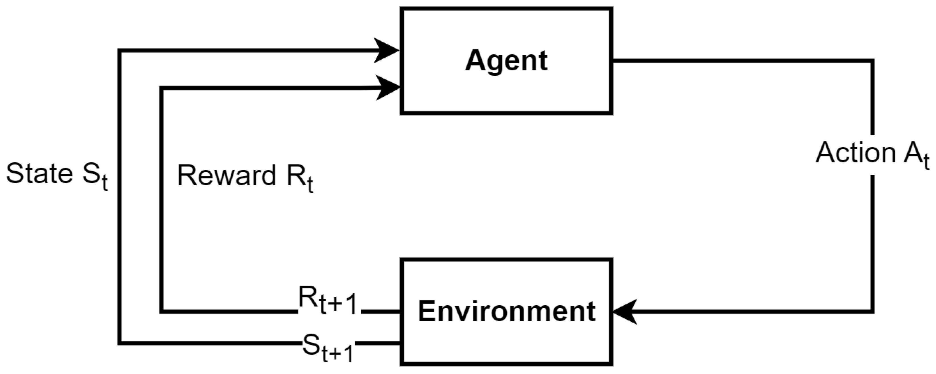
2.1. Markov Decision Process

Markov decision process (MDP) is a mathematical decision–making model where the action impact is partially random and partially controlled. Based on the definitions, we can mathematically formulate the probability of transitioning from state $S_t$ to state $S_{t+1}$ as:

$$P_{s{s}^{\prime }}^a=P(s^{\prime }\in S_{t+1}|S_t=s,A_t=a)$$

(1)

while the immediate reward can be formulated as:

$$R_a(s,s^{\prime })=R(s^{\prime }\in S_{t+1}|S_t=s,A_t=a)$$

(2)

where S is the set of states, A the set of actions, a the selected action in state s at timestep t, R the reward obtained by transitioning from state s to state $s^{\prime }$, with the selected action a. Simply put, $P_{ss\prime }^a$ is the probability of transitioning from the current state $s\in S_t$ to the next state $s^{\prime }\in S_{t+1}$, taking action $a\in A_t$, at time–step t in the transition of the process. MDPs can be either deterministic or stochastic. In deterministic approaches, as in every deterministic system, from state s, we can only transition to a unique state $s^{\prime }$, in contrast with stochastic approaches where s can lead to every possible state $s^{\prime }$. MDP is a structural element of RL since, in these problems, an agent is supposed to decide its next action based on its current state. In particular, when the above step is repeated over the time–step t, the problem can be expressed as an MDP.

2.1.1. Reinforcement Learning

In most RL algorithms, the agent obtains a model of the environment or at least some basic state transition sequences, as is depicted in Figure 1. In a similar model, the agent can interact with the environment by selecting a set of actions that alter the environment’s state, producing new states along the way. The structural components of RL are:

• The discrete different time–steps t;
• The state space S with state $S_t$ at time–step t;
• A set of actions A with action $A_t$ at time–step t;
• The policy function $\pi (.)$;
• A reward function $R_a(S_t,S_{t^{\prime }})$ of an action $At$, transitioning from state S to $S^{\prime }$;
• The state evaluation $V\left(s\right)$ and energy evaluation $Q(s,a)$.

2.1.2. Policy

In MDPs, the policy $\pi (.)$ is mathematically defined as a function with input value the state s from S and output value the action a from $A_S$.

$$\pi :S⟶A$$

(3)

According to MDPs in deterministic policy, the function $\pi (.)$ is defined as $\pi :S⟶A$, for each state $sϵS$ corresponds to one action $aϵA_s$ whereas in a stochastic policy, the function $\pi (.)$ is derived from the distribution of probability $\pi \left(a\right|s)$. In the latter case, the agent is able to choose one action $aϵA_s$, based on the distribution $\pi \left(a\right|s)$. During the training phase, the agent can act based on two policies:

• Exploration policy: The agent acts randomly to explore the state and the reward spaces.
• Exploitation policy: The agent acts based on preexisting knowledge.

2.1.3. State Evaluation

State Evaluation in MDPs is defined as $V:S⟶R$. To formulate it mathematically, it is important to also define:

• $\gamma$ the reward discount factor, which can take values between zero and one. The rate $\gamma$ pushes for immediate rewards;
• $G_t$ the reward sum (discounted by $\gamma$), from state $S_t$ until the end of the episode;
• $E_{\pi }$ the expected value of the rewards, given that the agent starts from the state s and acts based on policy $\pi (.)$.

$$V^{\pi }\left(s\right)=E_{\pi }\{G_t|S_t=s\}=E_{\pi }\left\{\sum _{k=0}^{\infty }{\gamma }^k{r}_{t+k+1}|S_t=s\right\}$$

(4)

where k is the number of steps before the end of the episode.

2.1.4. Energy Evaluation

The energy evaluation function can provide us with the expected discounted reward from $\gamma$, the sum of rewards that an agent can take if action a from a state s, based on a policy $\pi (.)$. It is defined as $Q:S\times A⟶R$.

$$Q^{\pi }(s,a)=E_{\pi }\left\{G_t\right|S_t=s,A_t=a\}=E_{\pi }\left\{\sum _{k=0}^{\infty }{\gamma }^k{r}_{t+k+1}|S_t=s,A_t=a\right\}$$

(5)

Taking into account the above function, a greedy deterministic policy can be:

$$V_{\ast }\left(s\right)=maxa\left\{Q_{\ast }(s,a)\right\}$$

(6)

2.1.5. Bellman Equations

Richard Bellman introduced a set of equations that help in solving MDPs [13]. They are extensively used both in RL and in the majority of the algorithms for solving game–based problems. To provide a proper mathematical definition of these equations, we must determine the probability of transition p and the expected reward R:

$$P_{s{s}^{\prime }}^a=P_r(S_{t+1}=s^{\prime }|S_t=s,A_t=a)$$

(7)

and

$$r(s,a)=E\left(r_{t+1}\right|S_{t+1}=s^{\prime },S_t=s,A_t=a)$$

(8)

With the above additions, we can reformulate both state and energy evaluation as:

$$V_{\pi }\left(s\right)=\sum _a\pi \left(s\right|a)\sum _{s^{\prime }}{P}_{s{s}^{\prime }}^a[r(s,a)+\gamma V_{\pi }\left(s^{\prime }\right)]$$

(9)

and

$$Q_{\pi }(S,a)=\sum _{s^{\prime }}{P}_{s{s}^{\prime }}^a[r(s,a)+\gamma \sum _{a^{\prime }}\pi \left(a^{\prime }\right|s^{\prime })Q_{\pi }(s^{\prime },a^{\prime })].$$

(10)

The importance of the Bellman equations is the fact that they let us describe the value of a state $S_x$ according to the value of another state $S_y$. This means that if we know the value of $S_{t+1}$, we can calculate the value of $S_t$. Thus, starting from a random initialization of the value function and retrospectively applying the Bellman equation, we can apply the energy evaluation function for all the possible states S and so calculate a new policy ${\pi }_{new}(.)$. Its policy-based recursion process can be seen in Figure 2.

2.1.6. Best Policy

The best policy satisfies the Bellman equations and returns the maximum sum of rewards reduced over time by $\gamma$. As the best policy ${\pi }^{\ast }$ of an MDP, we can define:

$$Q^{{\pi }^{\ast }}(s,a)\ge Q^{\pi }(s,a),\forall s,aϵS,A.$$

(11)

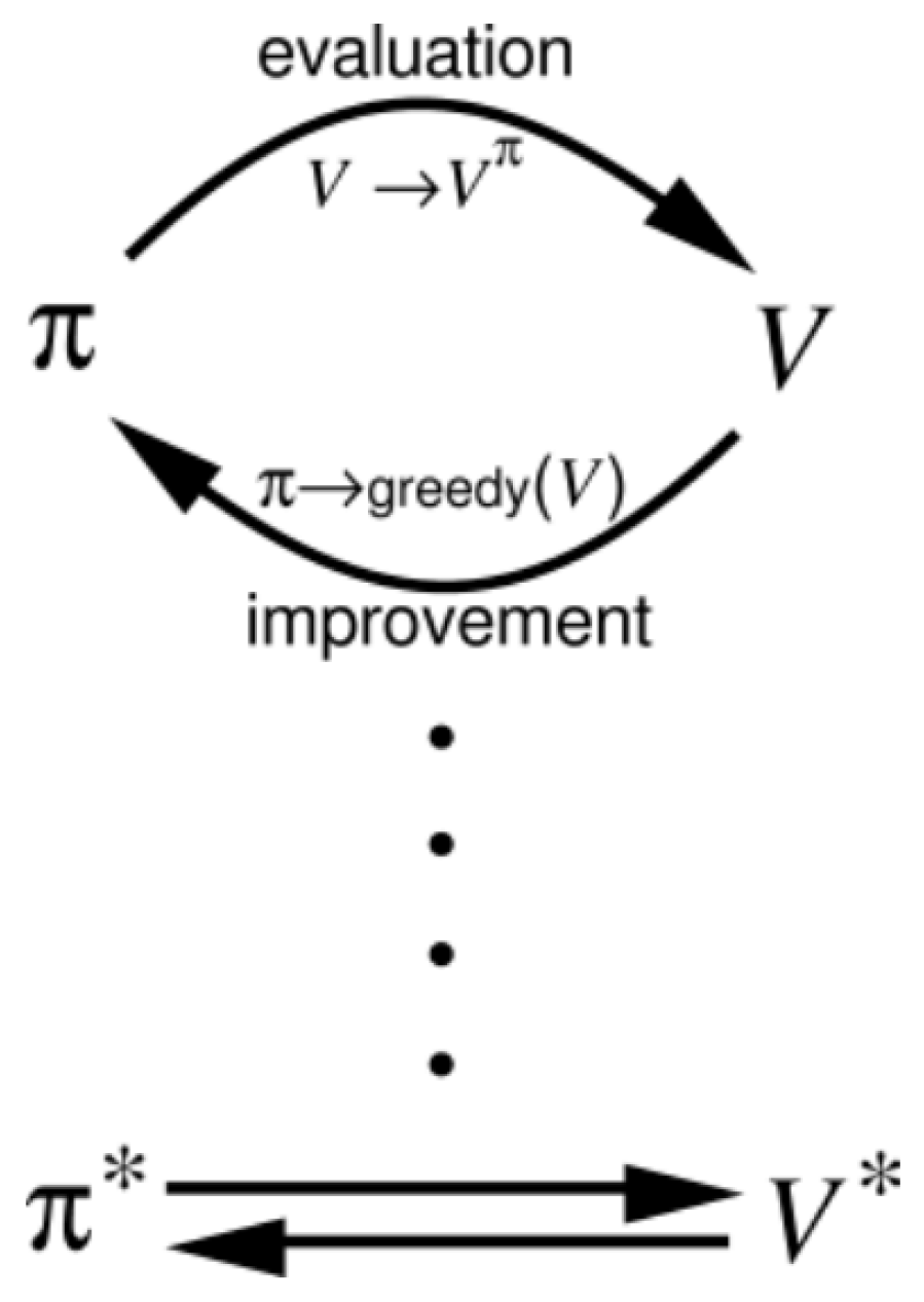
2.1.7. Policy Evaluation and Policy Improvement

Policy evaluation and improvement can be accomplished using dynamic programming algorithms, based on a value function. If the environment is known, a system of linear equations is set [22]. However, in this case, linear programming can be computationally expensive. Another family of RL algorithms that plays an important role in improving the above policies is the Monte Carlo method [23]. In contrast with linear programming, this method does not require extensive information about the complete environment. It is responsible for utilizing samples of state sequences, actions, and rewards. As RL problem solution concerns, the above method calculates the average of the observed rewards.

2.1.8. Temporal Difference Learning

Temporal difference learning (TDL) [24] is one of RL’s most popular and innovative concepts. It is a hybrid of dynamic programming and Monte Carlo simulations. TDL, like dynamic programming, adjusts its reward predictions depending on estimations the agent has already learned. Furthermore, it does not require substantial knowledge about the agent’s surroundings, but merely sequences of interactions, similar to Monte Carlo approaches. Because TDL approaches offer the aforementioned benefits over all other methods, they are widely employed in RL algorithms [17]. As a result, they are the most effective instrument for determining the appropriate policy. They can be employed with minimum computing expense, in the proper context, and, most significantly, with only one equation [25]. The techniques ($TD\left(0\right)$) are the simplest TDL approximation, using the following update rule:

$$V\left(S_t\right)⟵V\left(S_t\right)+lr[r_{t+1}+\gamma maxaV\left(S_{t+1}\right)˘V\left(S_t\right)]$$

(12)

where $0<lr<1$ is the learning rate, $r_{t+1}+\gamma V\left(S_{t+1}\right)$ is the target of the temporal difference, and $r_{t+1}+\gamma V\left(S_{t+1}\right)˘V\left(S_t\right)$ is the loss of the temporal difference.

2.1.9. Q–Learning Algorithm

One of the most well–known temporal difference (TD) algorithms is Q–learning (see Algorithm 1) [26,27]. Q–learning is an out–of–policy algorithm; therefore, its policy does not have to coincide with the evaluated and updated policy. It uses the following update rule:

$$Q(S_t,A_t)⟵Q(S_t,A_t)+a[r_{t+1}+\gamma Q(S_{t+1},a)˘Q(S_t,a_t)].$$

(13)

This algorithm approximates the best function $Q^{\ast }$, independently from the policy that the agent follows, as $\gamma maxQ(S_{t+1},a)$ refers to the best action the agent can perform being at state $S_{t+1}$.

Algorithm 1 Q–learning algorithm.

1: initialize $Q(S_t,A_t)$ 2: for every episode do 3:   observe state $S_t$ 4:   while $S_t$ in terminal do 5:     select action $A_t$ and evaluate Q 6:     take action a 7:     observe r, $S_t$ 8:     $Q(S_t,A_t)\leftarrow Q(S_t,A_t)+a[r_{t+1}+\gamma Q(S_{t+1},a)˘Q(S_t,a_t)]$ 9:     $S_t\leftarrow S_{t+1}$ 10:   end while 11: end for

So far, all these methods require intense memory allocations to work correctly. Specifically, we must keep s and a for every state $S_t$ and action $A_t$. A solution is impossible in real–world applications where the state space is vast. This is why reward functions need to be approximated with other types of functions, such as parametric [28]. Therefore:

$$Q(s,a)\approx Q_{\theta }(s,a).$$

(14)

3. Publication Analysis and Trends

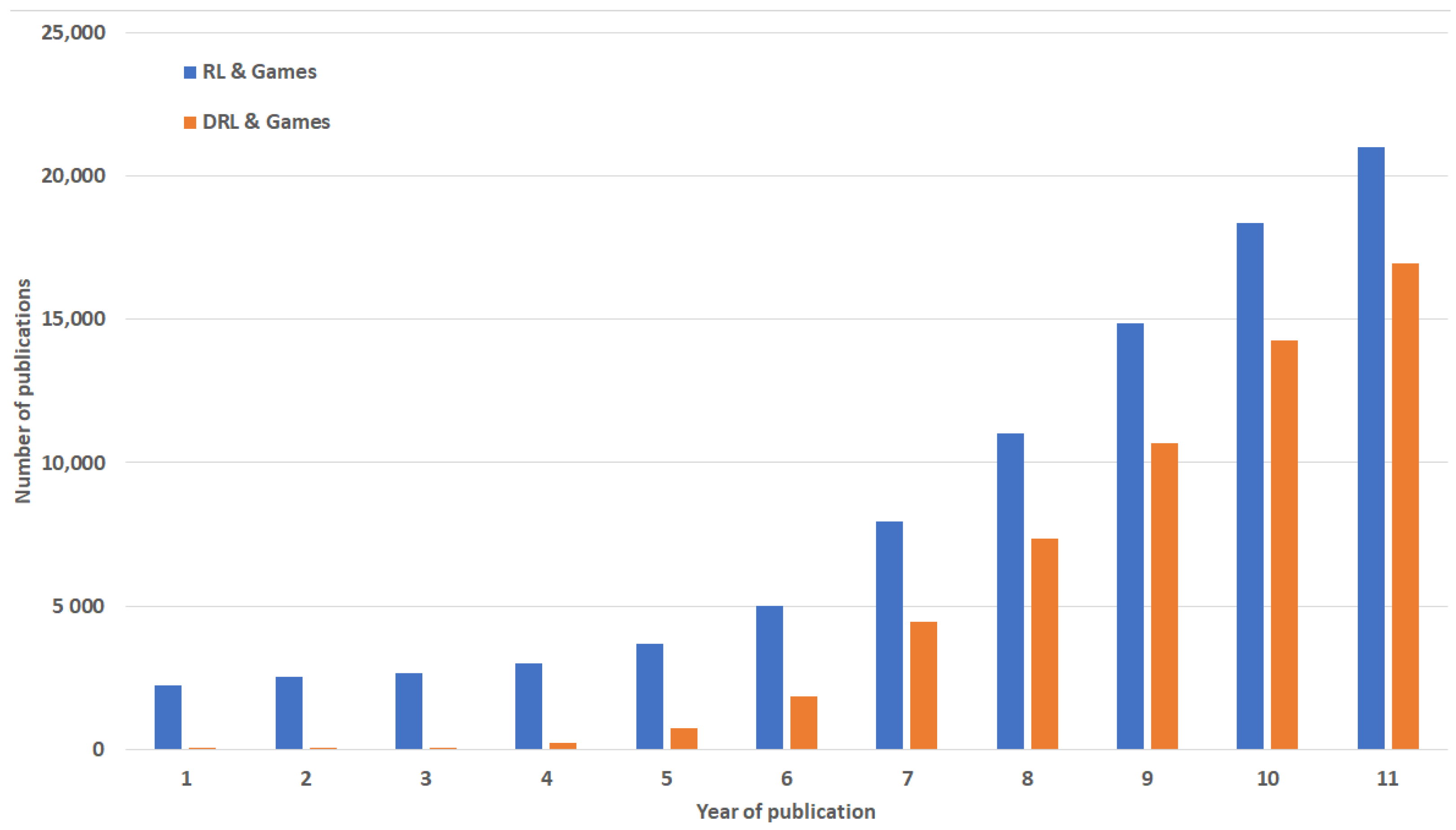
3.1. Statistics

So as to demonstrate the first argument, we examined Scopus (curated abstract and citation database, https://www.scopus.com/ (accessed on 20 December 2022), Google Scholar (search engine for scholarly literature, https://scholar.google.com/ (accessed on 20 December 2022)), and Dimensions (linked research information dataset, https://www.dimensions.ai/ (accessed on 20 December 2022)) publication/literature data for each year, searching for terms and keywords such as “deep reinforcement learning,” “games,” “reinforcement learning,” and “deep learning,” as illustrated in the corresponding graph (Figure 3).

More specifically, the total publication (proven research) count for the jointed terms “reinforcement learning” and “games” was 92,367 for the time interval 2012–2022, and the publication count for the jointed words “deep reinforcement learning” and “games” was 56,613 for the period 2012–2022.

For the second point, we examined the period 2012–2022, utilizing publication data from Scopus, Google Scholar, and Dimensions focusing on the broader fields of “deep reinforcement learning” and “reinforcement learning”. For the terms and keywords “reinforcement” and “learning” and “games”, 92,367 findings were reported between 2012 and 2022. From our previous 2018–2022 findings, we observed that 73,245 results had been released, accounting for almost 73% of all publications.

To summarize, the recent trend in RL–based research on games has focused on DL approaches. Specifically, several methods from genetic programming (GP) demonstrate competitive results on ALE, ViZDoom, StarCraft, and Dota 2, which actually indicate the converse, meaning that the computational cost of deploying DL solutions to such games is considerably higher than GP [29,30,31,32]. This arises from the fact that conventional methods have substantial memory and calculation complexity drawbacks. DL has overcome these limitations because of its ability to handle such multidimensional data and its scalability. The same diagram in Figure 3 also depicts the research activity related with the terms and keywords “deep”, “reinforcement”, “learning” and “games” in the time interval 2012–2022, as well as the keywords “reinforcement”, “learning” and “games” in the period 2012–2022, relative to the publication count [14].

3.2. Trends

The literature on the subject of deep RL revealed various patterns linked to specific game titles [33]. For some earlier titles, the results were created using “deep reinforcement learning” or “reinforcement learning”. ATARI games, in particular, have piqued the scientific community’s curiosity, followed by board games (almost half of which are “Chess”) and some newer multiplayer online battle arena (MOBA) or strategic games.

The following sections analyze the role of each deep RL component in each game. As a result, the study focuses on these six game “trends” regarding game titles, attaching a little more importance to ATARI [34].

3.3. Deep Reinforcement Learning and Games

3.3.1. Transition to Deep Reinforcement Learning

Humans can perceive patterns and complete complicated tasks in a very short period. Inside this framework, they successfully interpret optical data, transcribe them into meaningful entities, process them, and eventually make intelligent judgments. Over the last few decades, the scientific community has made significant efforts to accomplish these crucial human capabilities. Even before the turn of the century, studies suggested that intelligent algorithms that could adapt/learn from data may be used to solve this problem [35]. The most widely accepted explanation is that it works similarly to the human brain and central nervous system. These “brain modelling” algorithms can adapt to various problems. They were, however, hampered by the lack of computationally powerful equipment at the time. At its pinnacle, the family of theories, methods, and algorithms based on this principle was known as “neural networks”, and it was considered to be the top choice in most problem–solving domains [36]. Over the last ten years, vast and parallel computing capability has allowed us to tackle exceedingly complicated, fundamental issues in a short period and often outperform humans. Reinforcement learning welcomed this new potential, extending unsupervised learning’s limitations further and morphing into a new area known as “deep reinforcement learning.”

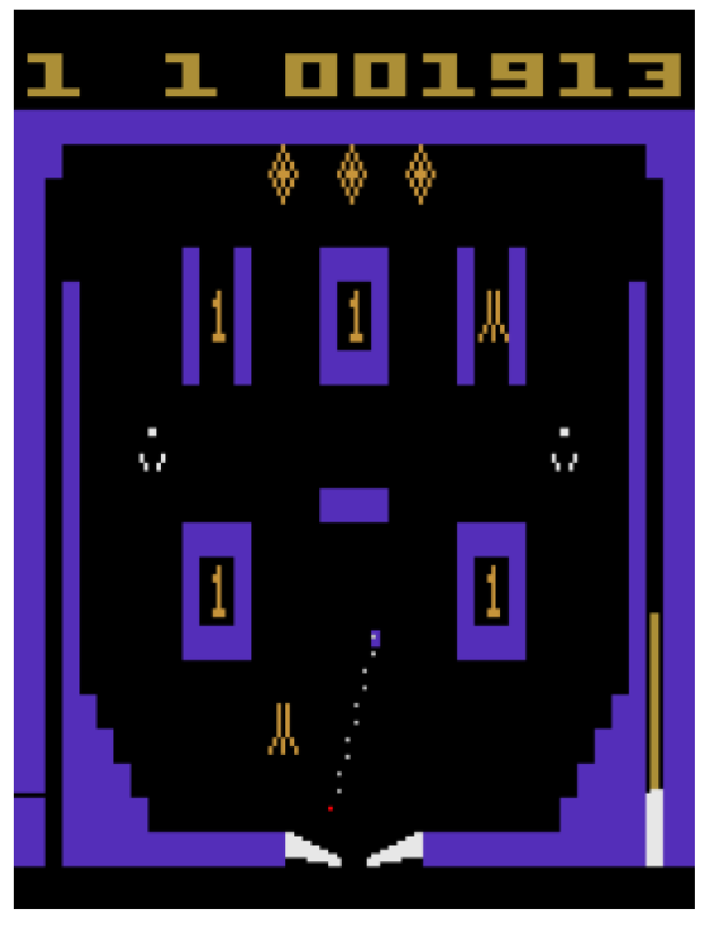
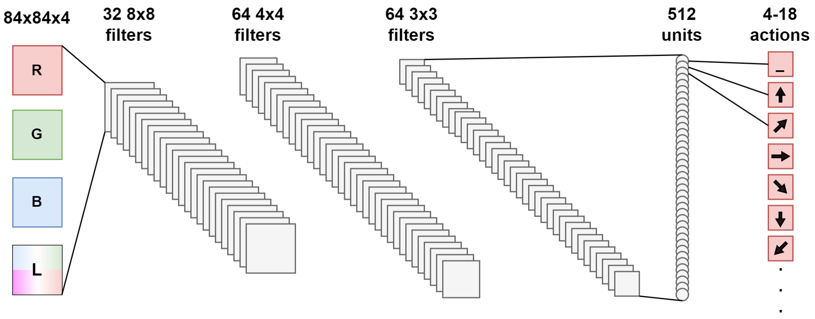
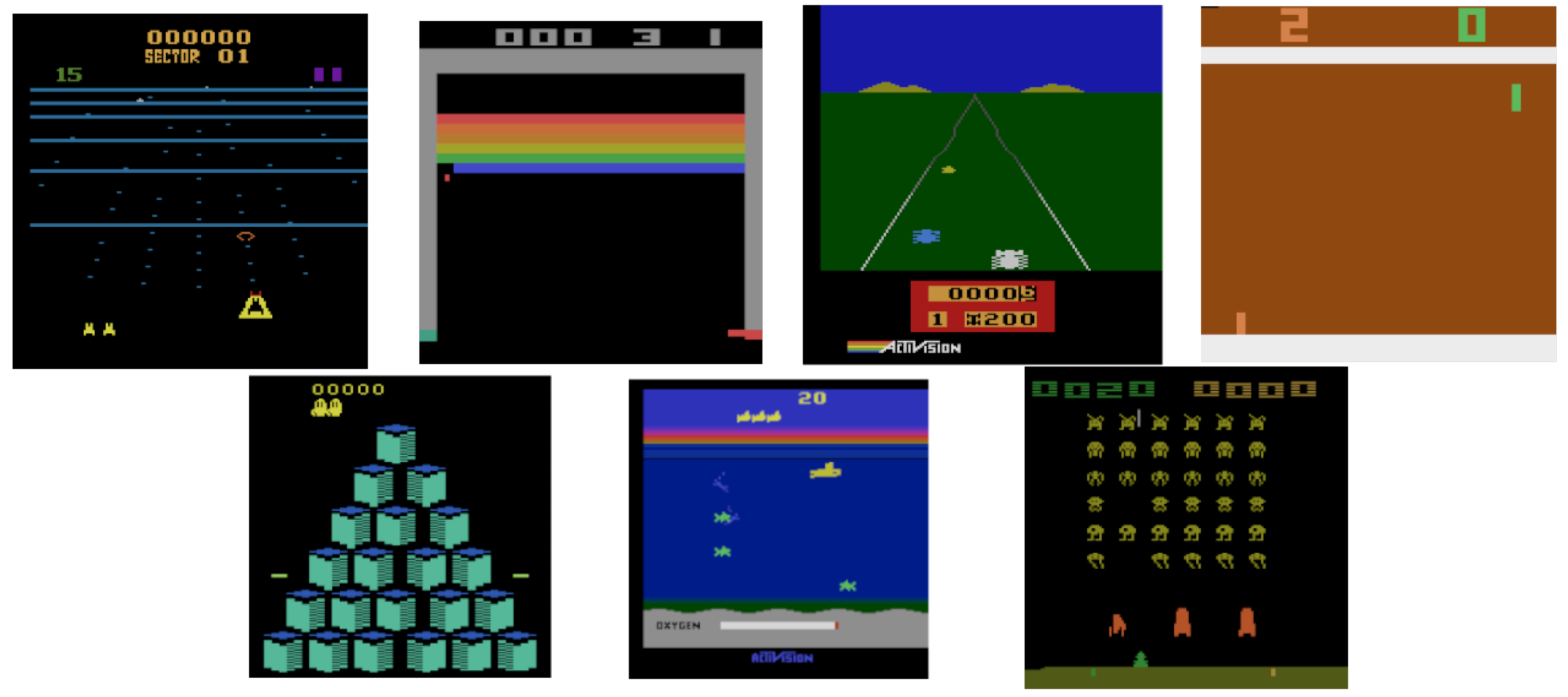
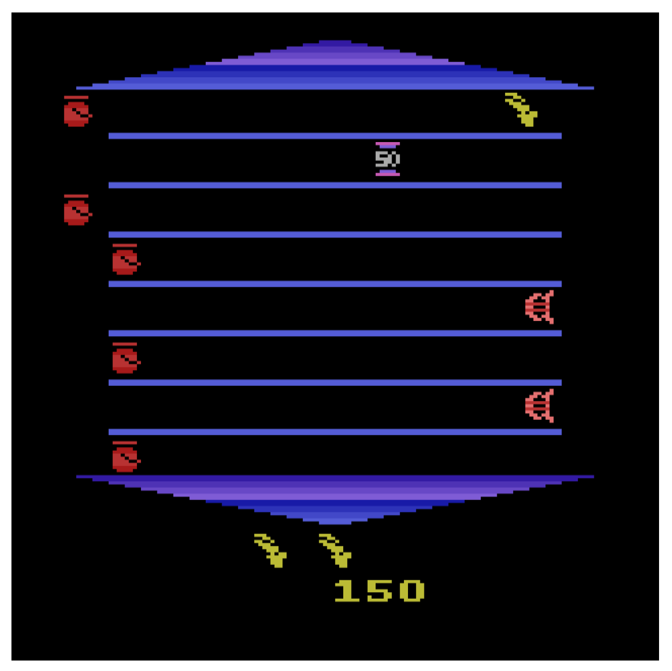
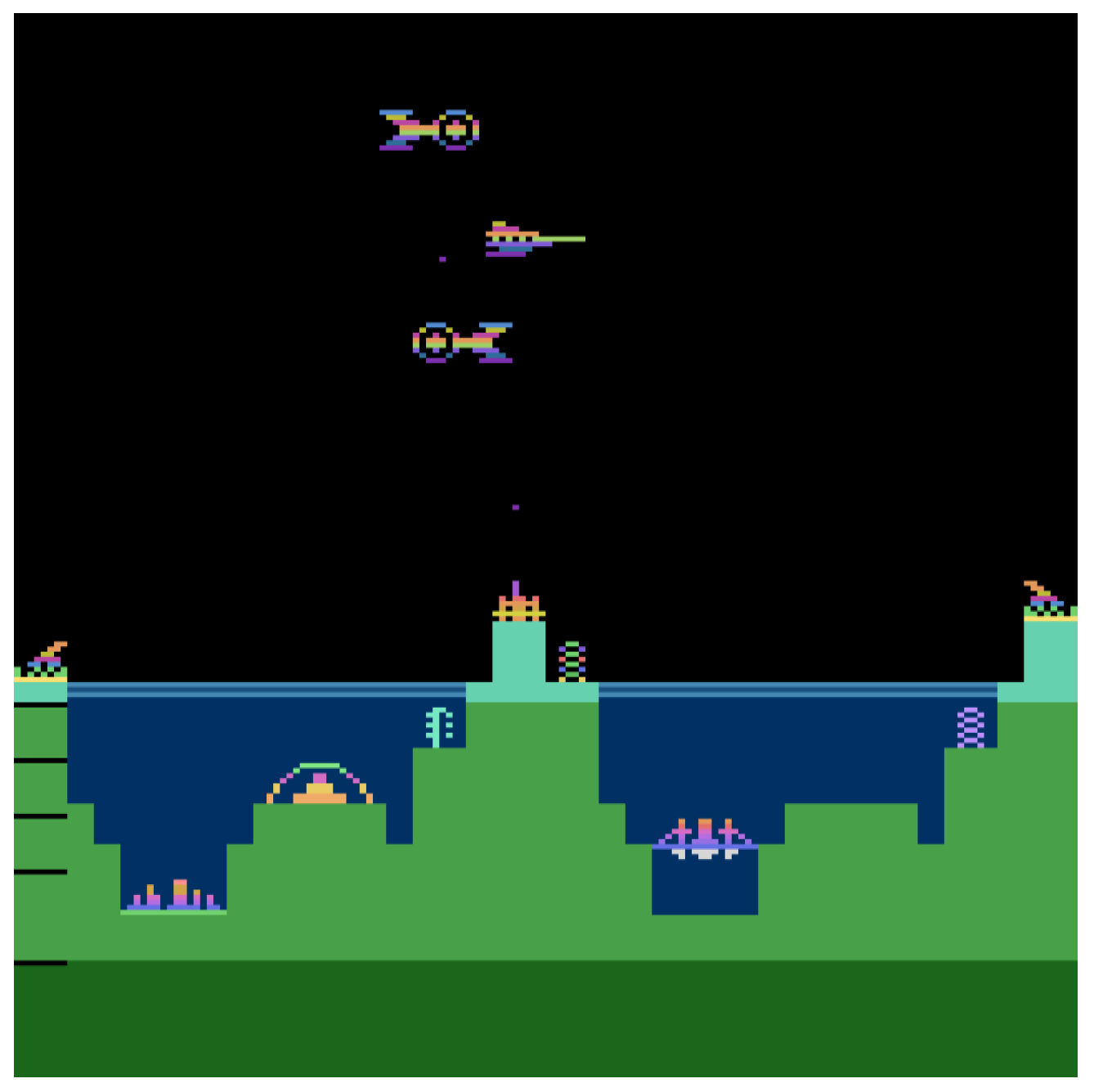
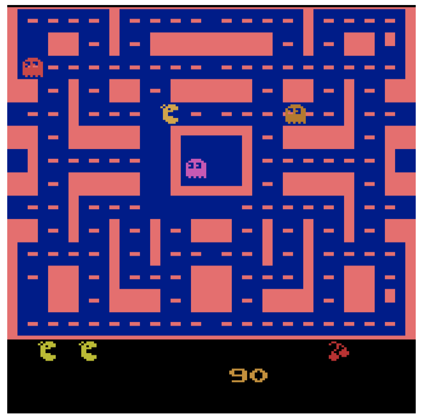
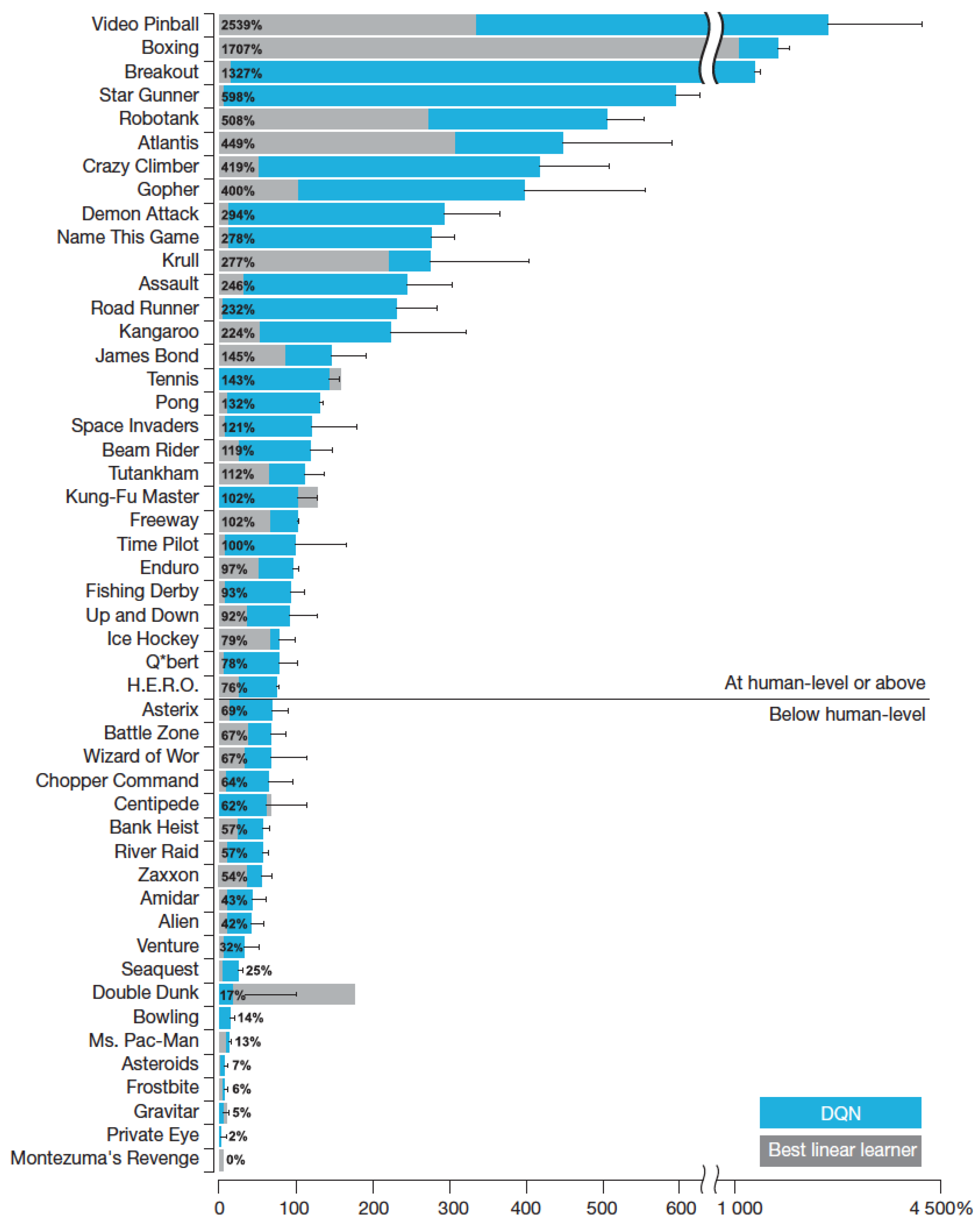
3.3.2. Deep Q–Network in ATARI

According to [19] that DeepMind published in February 2015, the combination of deep neural networks (DNNs) with classic RL methods was described. The results in games of the ATARI console were excellent (high score in the famous breakout game; see Figure 4).

There are several games in which superhuman–level performance has been achieved. DQN can represent states using deep convolutional neural networks (CNNs) to reduce the complexity, which in real–world problems is prohibitive using the classic methods, as analyzed in the previous section. The architecture of the network is illustrated in Figure 5. More specifically, the architecture of the DQN was consisted of a 4–dimensional 84 × 84 input image that included the RGB channels of the game’s current frame, along with the luminance channel. The input layer is then followed by three convolutional layers with 32 8 × 8 filters with a stride of 4, 64 4 × 4 filters with stride of 2, and 64 3 × 3 filters with stride of 1, respectively. Moreover, the first and second convolutional layers also applied a rectifier nonlinearity, whereas the third one was followed by a simple rectifier. The final layers consisted of a fully connected dense layer with 512 units, followed by the output layer that consisted of a single output for each of the 4–18 valid actions, considering the “no action” as well.

The expected result is that the agent will be capable of interacting with the rest of the environment with actions, observations, and rewards [39]. Therefore, the agent’s target is to choose which actions will maximize its rewards. In this case, in particular, the deep neural network (DNN) tries to approximate the best energy evaluation function:

$$Q(s,a)=maxE[r_t+{\gamma }^2{r}_{t+2}+\dots |S_t=s,A_t=a,\pi ].$$

(15)

RL is not predictable from the beginning or even deviates when a nonlinear function approximation, such as NNs, is applied to estimate the energy evaluation function. The correlation in sequence observations, as well as the one between energy values and the TD target and the fact that tiny changes in the energy value function would result in many substantial changes in the agent’s policy [40], contribute to the turbulence. DQN, a variation of the Q–learning method that utilizes two core principles, was developed by DeepMind to solve this instability. Initially, an experience replay (experience repetition) mechanism was used, which chose random observations for learning and thereby eliminated the association between a sequence of observations [41].

The second idea was to shift the energy value function in the direction of the TD goal  [42,43], but only periodically rather than after each observation, thereby diminishing the relationship between the two. This is performed by regularly replicating the Q network into a second Q network, which is used to estimate the TD target and update the Q–network parameters [44].

The neural network (NN) shown in Figure 5 was used to configure an estimated value function of energy $Q(s,a|{\theta }_i)$ in the DQN implementation, where ${\theta }_i$ is the parameter (i.e., the weights) of the Q–network in iteration i. Agent “experience” is then processed in quads $e_t=(S_t,A_t,r_t,S_{t+1})$ to enforce experience repetition. At any time t during training, the energy value function’s values are renewed based on samples of experiences randomly selected from the stored data collection. This update is based on the derivative convergence algorithm (gradient descent) and uses the following function error:

$$L\left({\theta }_i\right)=E{(s,a,r,s^{\prime })}_{\sim U\left(D\right)}\left[{(r+\gamma maxQ(s^{\prime },a^{\prime }|{\overline{\theta }}_i)˘Q(s,a|{\theta }_i))}^2\right]$$

(16)

where $\gamma$ is the discount factor (or rate) that defines the agent’s “visibility”, ${\theta }_i$ is the Q–network parameters in iteration i, and ${\overline{\theta }}_i$ is the parameter of the $\overline{Q}$–network used to measure the TD goal in iteration i. The parameters ${\overline{\theta }}_i$ are modified every C iterations by copying the parameters, and they remain stable between their renewals [45]. The algorithm is also shown in Algorithm 2.

Algorithm 2 Deep Q–learning algorithm.

initialize replay memory 2: initialize value function     initialize target value function 4: for every episode do       initialize sequences 6:   for $t=1,T$ do         select random action $A_t$ 8:     otherwise select $A_t=arg\; maxQ(\Phi \left(S_t\right),a|\theta )$         execute action $A_t$, observe reward $r_t$ and image $x_{t+1}$ 10:     set $S_{t+1}=S_t,a_t,x_{t+1}$         preprocess ${\Phi }_{t+1}=\Phi \left(S_{t+1}\right)$ 12:     save transition ${\Phi }_t,a_t,r_t,{\Phi }_{t+1}$         pick new random transition ${\Phi }_t,a_t,r_t,{\Phi }_{t+1}$ 14:     set $y_j$         perform Gradient Descent to the ${(y_j˘Q({\Phi }_j,a_j|\theta ))}^2$ 16:     reset the approximation $\overline{Q}=Q$       end for 18: end for

DeepMind used this technique (DQN) to train video data, incentives, terminals, and accessible moves for ATARI games [46]. The network was not given any fundamental knowledge about the game and was trained using video data, rewards, terminals, and accessible movements. This is how a typical user would approach it. Its purpose was to create a single neural network agent that could train (and play) many games. In six of the seven games, the DeepMind Technologies agent defeated every other algorithm with DQN while also beating the world record set by human players in three of them (see Figure 6) [41].

3.3.3. Double Q–Learning

Even though double Q–learning (shown in Algorithm 3) and DQN were watershed moments in the world of RL, they had some flaws. Many researchers suggested improved versions to address these problems [48]. DeepMind also made further improvements regarding the deep Q–learning algorithm and the network, achieving even more excellent high scores in ATARI games such as pinball, as shown in Figure 4. Double Q–learning is the first significant improvement of the initial algorithm.

Algorithm 3 Double Q–learning algorithm.

initialize $Q_A,Q_B,s$     for every episode do 3:   choose a related with $Q_A$ and $Q_B$       observe $r,s^{\prime }$       choose at random UPDATE(A) or UPDATE(B) 6:   if UPDATE(A) then         Define $a^{\ast }=arg\; max{Q}_A(s^{\prime },a)$         $Q_A(s,a)\leftarrow Q_A(s,a)+a(s,a)(r+\gamma Q_B(s^{\prime },a^{\ast })˘Q_A(s,a))$ 9:   else if UPDATE(B) then         Define $b^{\ast }=arg\; max{Q}_B(s^{\prime },a)$         $Q_B(s,a)\leftarrow Q_B(s,a)+a(s,a)(r+\gamma Q_A(s^{\prime },b^{\ast })˘Q_B(s,a))$ 12:   end if     end for

Hado van Hasselt explains that the Q–learning algorithm does not perform well in specific stochastic environments [49]. This occurred due to overestimating the energy values using $maxQ(s^{\prime },a)$. The suggested solution was to hold two Q–value functions, $Q_A$ and $Q_B$, which are renewed for the next state by each other. The renewal is carried out by first determining the energy $a^{\ast }$ that maximizes $Q_A$ in the following state:

$$Q(s,a)=maxQ(s^{\prime },a)$$

(17)

and then calculating the value of $Q_B(s,a)$ based on $a^{\ast }$ so that the renewal in $Q_A$ can be carried out as $Q_A(s,a)$.

This particular technique can be combined with DQN, boosting its capabilities, by using the following loss function:

$${[R_{t+1}+{\gamma }_{t+1}{q}_{\theta }(S_{t+1}arg\; max{q}_{\theta }(S_{t+1},a^{\prime }))˘q_{\theta }(S_t,A_t)]}^2.$$

(18)

This modification was shown to reduce the overestimation of energy values in the DQN algorithm, resulting in improved algorithm efficiency.

3.3.4. Prioritized Experience Replay

According to the replay buffer technique, the DQN algorithm selects samples from memory. However, it would be preferable to use samples from state transitions that are crucial in training. Tom Schaul [50] presented the concept of priority inexperience in 2015. The idea is to choose experience samples with a significant difference between them at the approximate value of Q and the TD target, as this means that these particular experiences “carry” much information. The transitions––experiences are chosen with a probability of p based on the last occurrence of an absolute error:

$$p_t{|R_{t+1}+{\gamma }_{t+1}max\overline{q_{\theta }}(S_{t+1},a^{\prime })˘q_{\theta }(S_t,A_t)|}^{\omega }$$

(19)

where $\omega$ is a hyperparameter that defines the shape of the distribution. Finally, new experiences are added to the memory with the highest priority, giving recent transitions precedence.

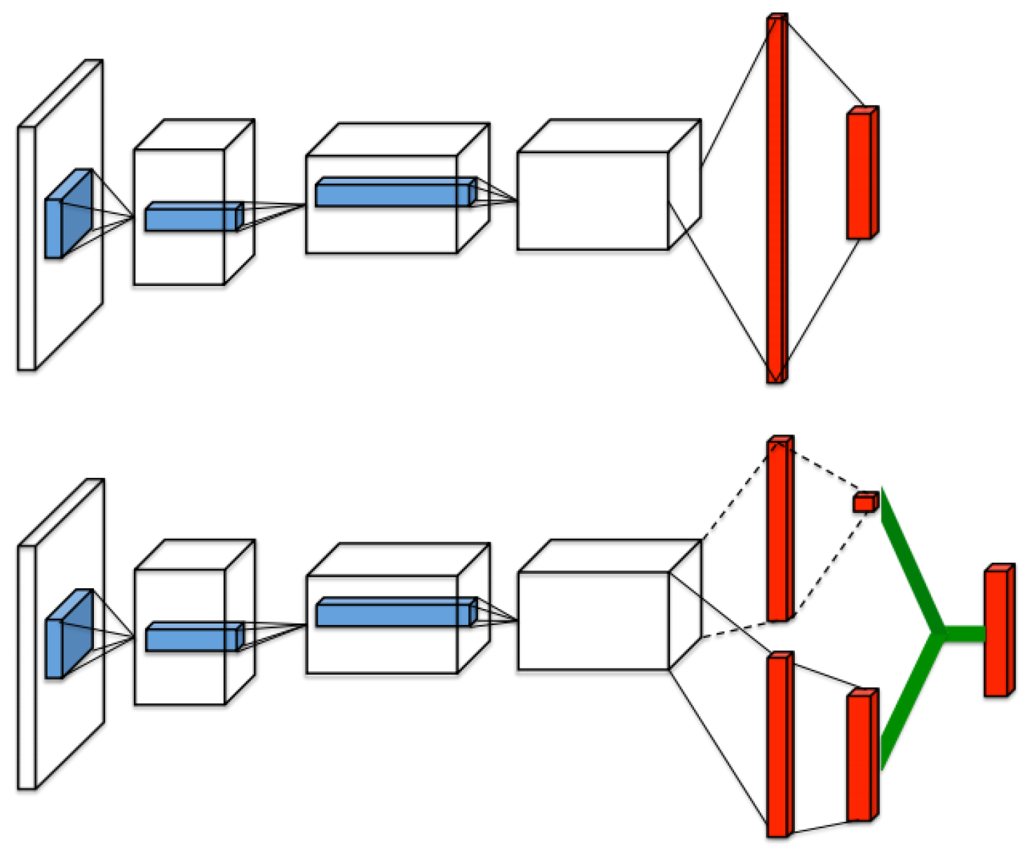
3.3.5. Dueling Networks

Dueling Network architecture is based on the idea that assessing the value of each possible action is not always essential. Knowing which energy should employ would be critical in certain situations, but the energy choice has the minimum impact on the outcome in many others. However, estimating the relevance of the states is necessary for bootstrapping methods.

To obtain this discovery, Google DeepMind created the Dueling Network [14]. The lowest layers are convolutional, as they were in the DQNs [51] at the time. They employ two sequences (or streams) of ultimately linked layers instead of utilizing coherent layers followed by a single sequence of fully connected layers. The streams are set up to produce independent estimations of value and reward functions. Finally, the two streams are combined to provide only one Q mode output. There are Q values in the network output, one for each service. Because the Dueling Network’s performance is a Q function, it may be trained using several techniques, including DDQN and SARSA [52]. It will also benefit from improvements to these algorithms, such as improved repetition memories and exploration strategies. The module that combines the two streams of completely connected layers to generate a Q rating necessitates meticulous design.

It is worth noting that Q values indicate how profitable it is for the agent to be in state s and take action a ($Q(s,a)$) as shown in the function below:

$$Q(s,a)=A(s,a)+V\left(s\right)$$

(20)

where $V\left(s\right)$ is the agent’s value for being in state s, and $A(s,a)$ is the advantage of the agent choosing energy a in state s (how much better the outcomes would be if this action were chosen, over all the possible actions).

There is a need to isolate the estimator of these two components using two new streams in conjunction with DQN:

• One that calculates the state value $V\left(s\right)$;
• One that will estimate the advantage of each action a in state s, $A(s,a)$.

Finally, the two estimators are combined through an aggregation layer to obtain $Q(s,a)$. Figure 7 portrays the network architecture. This distinction was chosen as all potential actions will lead to a negative outcome in some instances. Consequently, there is no need to compute the values of all potential actions in that case. As a result, we can only measure $V\left(s\right)$, which is particularly useful in circumstances where all actions have little or no impact on the environment. The entire procedure corresponds to the following energy value factorization:

$$q_{\theta }(s,a)=v_n(f_{\xi }\left(s\right),a)˘\frac{\sum (a^{\prime })a_{\psi }(f_{\xi }\left(s\right),a^{\prime })}{N_{actions}}$$

(21)

where $\xi ,n,\psi$ are the parameters of the convolutional decoder $f_{\xi }$, the value stream $v_n$, and the advantage stream $a_{\psi }$, and $\theta =\xi ,n,\psi$ is the set.

To summarize, DeepMind outperformed the competition in the majority of ATARI games using the new dueling Q–network architecture, with notably higher high scores (compared to old DQN) in Asterix (shown in Figure 8) and Atlantis (shown in Figure 9) games (in comparison with Double DQN). Except for Bowling, where the top scores attained decreased by 1.89%, dueling DQN was more successful in all other ATARI games. Of course, not all ATARI games benefited from this attempt to enhance training. Examples include Pinball (72.10% reduction) and Freeway (absolute reduction, i.e., 100%).

In the games Atlantis (as illustrated in Figure 9), Tennis, and Space Invaders, dueling DQN outperformed ordinary DQN by more than 100%. It is crucial to remember that each game is unique. As a result, the earlier DQ learning algorithm outscored even the more powerful DQN architecture in certain games. Ms. Pacman is a classic example of a game in this setting.

3.3.6. Microsoft’s Success

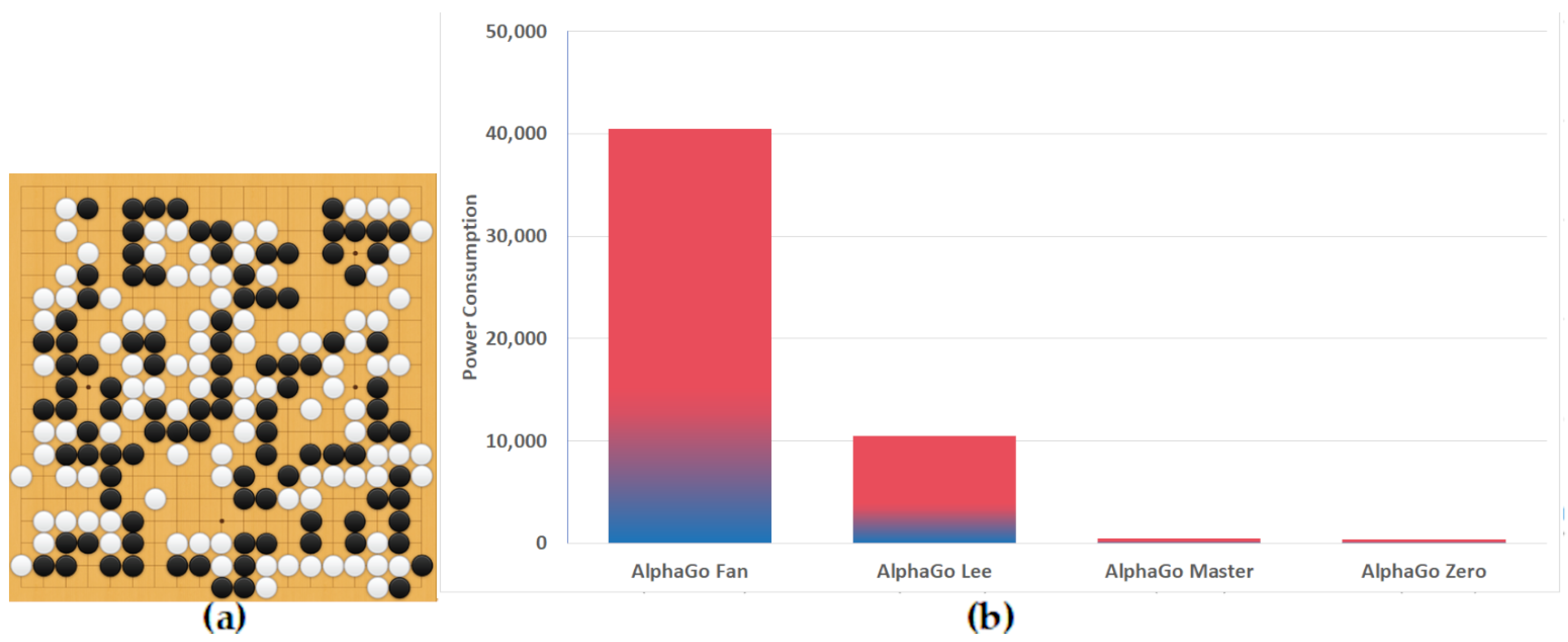
In June 2017, Microsoft reported that it had reached the highest possible score to be accomplished, despite continuous training failures of the Ms. Pacman game, both from Google using neural networks and other companies using different approaches. This phenomenal score of 999,990 was obtained by people cheating at the time. According to Twin Galaxies, a man’s highest score is 933,580, which belongs to Abdner Ashman.

This success came relatively late, as previous years saw substantial performances in other more challenging games, as described in the previous section. Beyond that, DeepMind’s AlphaGo has defeated human Go experts, while Libratus and DeepStack also easily defeated some poker professionals in heads–up no–limit Texas Hold’em. The A team from Maluuba used artificial intelligence (AI) to build tasks, broke them down into roles, and delegated them to over 150 agents. The hybrid reward architecture was used–––a mixture of enhanced learning and a divide and conquer algorithm. Every agent had different responsibilities (for example, finding a particular pill from the Ms. Pacman grid), which they shared with other agents to achieve better results. Another agent was then used that took into account all of the roles presented to each agent and decided which move Ms. Pacman would take.

The best results were obtained when each agent behaved entirely selfishly, and the super–agent concentrated on the best move for the entire club. This was achieved by assigning weights to the various options based on their relevance. For example, fewer agents attempt to stop ghost–enemies than those attempting to make the Pacman gain more points. There are four agents for ghost–enemies (one for each ghost–enemy) and four for chased ghosts. If the super agent’s decision were based on what the majority wanted, it would undoubtedly end up with a ghost enemy and lose. According to Harm Van Seijen, [53], there is significant importance in how agents should collaborate based on their options and how they should behave selfishly based on each agent’s only competence. This relationship benefits the entire process.

The method also employs RL, in which each behavior leads to a positive or negative reward, resulting in agents learning by trial and error. Over 800 million frames of the game were used to train the mechanism in total. Earning more points is less probable because it resets back to zero when the score hits one million points, as can be seen in Figure 10. Microsoft reaches the high scores in Pacman writing history.

3.3.7. AlphaGo

AlphaGo is an RL algorithm created by Google DeepMind and implemented to play the Go board game. It was the first algorithm capable of defeating a professional Go player on a full–size 19 × 19 game board [54]. In a series of best–of–five games in March 2016, the AlphaGo algorithm won the title against professional player Lee Sedol. Although Sedol won the fourth game (Figure 11a), he resigned in the third game, making the final score 4–1 in favor of AlphaGo.

AlphaGo employs the Monte Carlo tree search algorithm (MCTS), combining branching machine learning approaches with intensive human and computer games training. DL networks are also utilized, getting as input a description of the game board in every state s, passing it through different layers (hidden layers). Subsequently, the policy network chooses the next optimal action (for the computer player), and the value network (or evaluation) estimates the value of the current state s.

AlphaGo Zero is a recent AlphaGo development, which, unlike AlphaGo that learned to play professionally through thousands of games with novice and professional players, is learning by playing against itself. In just a few days, the agent accumulated thousands of years of human experience with the assistance of the best player in the world, none other than AlphaGo itself. AlphaGo Zero succeeded quickly and outperformed all of its previous versions.

There is a single NN during the game that knows nothing about Go at first. Eventually, the algorithm ends up playing with itself, combining the DNN with a robust NN search algorithm regulated and updated to assess movements. The updated network is combined with the same algorithm once more, and a stronger Zero emerges. This process is repeated many times, with each iteration increasing the system’s performance by a small percentage. Furthermore, Zero employs a single NN that combines the logic of the two policies and value networks presented in the initial implementations. As a result of these changes, Zero evolved in terms of algorithmic power and better computing power management. The graph in Figure 11b compares power consumption as a percentage of thermal design power (TDP) to previous AlphaGo implementations. AlphaGo Zero uses only 4 TPUs, making it, along with AlphaGo, the most power–efficient system for this task.

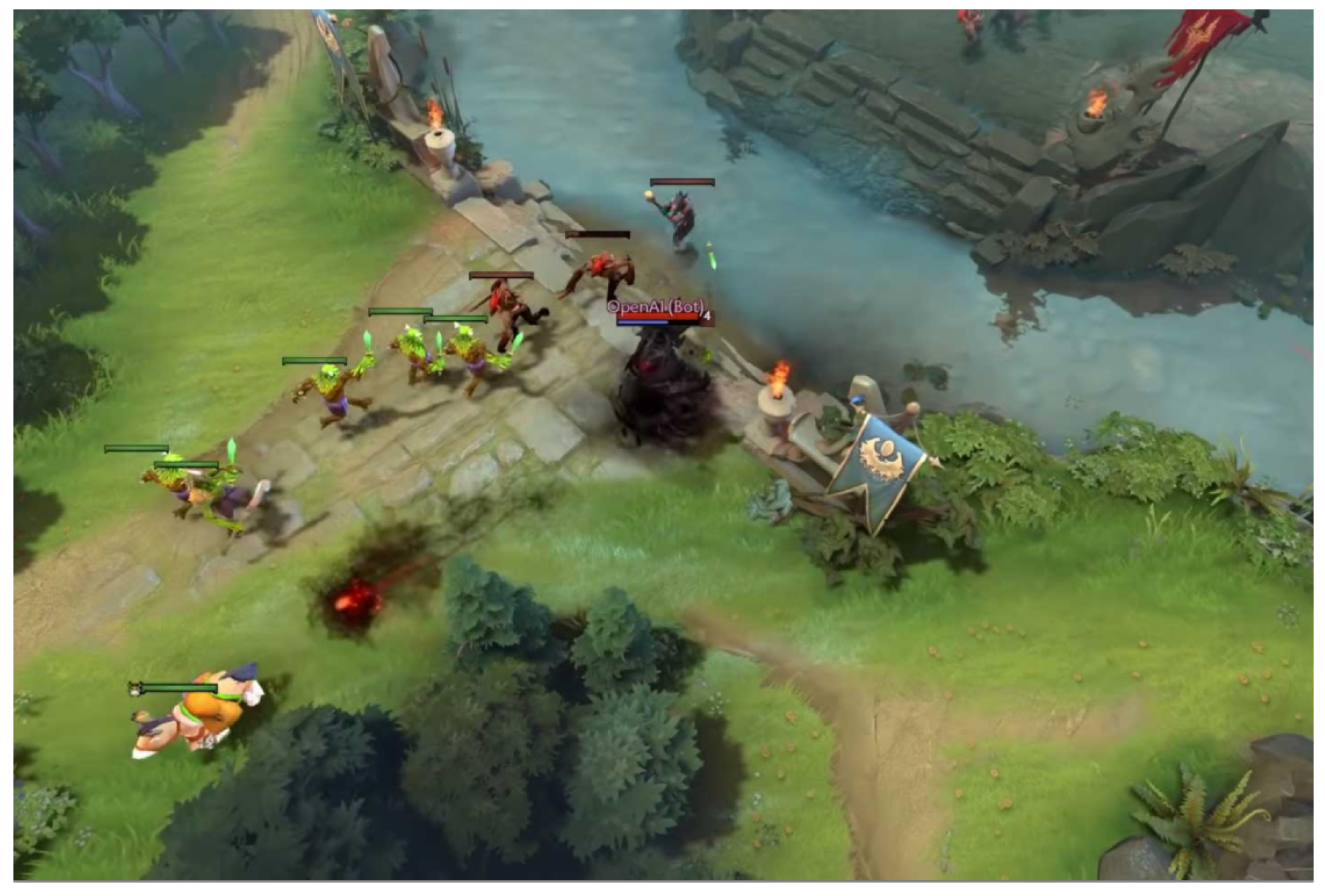
3.3.8. OpenAI Five in DOTA2

Dota 2 (https://www.dota2.com/home, accessed on 20 December 2022) is a MOBA game that is known, among other games in the same genre, for being a highly challenging video game, due to the large number of moves the player has in their hands (action space), the various calculations needed, and the multiple goals during a match. Figure 12 shows a snapshot during a game of Dota 2. The players, such as the units, are only visible in some areas of the world, making the environment partially visible (partial observability). This deep and nuanced style of play necessitates a steep learning curve. In 2019, OpenAI Five [55] succeeded in overcoming this difficulty by winning the OpenAI Five Finals in a five agents vs. the world champions match. Five consisted of five NNs that observe the game environment as a list of 20,000 numbers (input) encoding the observable field of play and function by selecting moves from an 8–number list [56].

The game’s general concept was based on the fact that the player is self–taught, beginning with random parameters and using a modified version of the PPO algorithm [55]. Each of the five team’s NNs is a single long short–term memory (LSTM) network [57] with 1024 units that obtains game status through a Bot API and exports moves with semantic value. For example, this value is counted in the number of ticks (unit of measurement used in game production that expresses how long one step takes) required to postpone the given motion in the X and Y coordinates surrounding the section where the movement will be performed, and so on. Each NN calculates its own movements, which means each agent makes its own decisions based on the current match goal and whether a teammate agent requires assistance. OpenAI Five was able to interpret conditions considered risky, such as the drop of ammunition in the region where the agent was put, using sufficient reward arrangement (reward shaping) and taking into account measurements, such as the fall and its health. The system was able to adapt to advanced gaming practices such as team play pressure on the opponent’s area (5–hero push) and stealing vital items (bounty runes) from the opponent after several days of practicing, with 80% of the time spent playing against himself and 20% against previous models. In a strategy setting such as Dota 2, the idea of exploration is also challenging. During training, properties such as health, speed, and the agent’s initial level were obtained at random values to force the agents to explore the environment strategically.

After losing many 1 vs. 1 battles against a single experimental player, the random training values were increased, allowing the system to start winning. OpenAI Five does not have a direct contact channel between agents and players regarding collaboration. A hyper–parameter is used to monitor how well they fit together. This hyper–parameter takes values ranging from 0 to 1 and calculates how heavy their individual reward is versus the average value of a group reward function.

3.3.9. AlphaStar in StarCraft II

StrarCraft II (https://starcraft2.com/en\T1\textendashus/) (accessed on 10 December 2022) is also an real time strategy game of high complexity and competitiveness, is regarded as one of the games with the most hours of esports competitions, and is a significant challenge for AI research teams. There is no right technique when it comes to being playful. The environment is again partially observable, while the agent must explore it. The amount of space available for movement is determined by two factors. Numerous manageable components result in many combinations [58].

Google’s DeepMind unveiled its 2019 AlphaStar implementation, the first AI to defeat Grzegorz Komincz, one of the best StarCraft II players, in a series of experimental races held on 19 December 2019, under professional classification match conditions, with a score of 5–0 in favor of AlphaStar [13].

This particular AI employs DL, RL techniques, and DNNs and accepts raw game data as input in the StarCraft II setting. These data are interpreted as a list of available sections and properties, and it outputs a collection of commands that comprise the movement performed at each time level. DeepMind called this architecture Transformer, which is based on attention mechanisms distributed using recurrent neural networks (RNNs) and CNNs [55]. The Transformer’s body utilizes one deep core LSTM, a strategy of self–regulating tactics, followed by an indicator network [59] and an approximation of an assessment aggregate value [60].

AlphaStar employs a multidisciplinary algorithm preparation. The network was initially trained using supervised learning by observing people playing games and imitating their short–term and long–term strategies. The training data were then used to power a multi–agent framework. For this technique, they conducted 14 consecutive days of confrontations with competing agents in a competition consisting solely of AI agents, where new entrants, who were branches of existing agents, were dynamically introduced. Each agent was given the goal of defeating either one or a group of opponents. The agents learned from the matches, which enabled them to explore a vast space of strategies related to the way StarCraft II plays while also ensuring that each contestant worked effectively against stronger strategies and did not forget how to face the weakest older strategies.

Such an approach is not dissimilar to how people invent new and improved tactics while dismissing the old ones as obsolete. The weights of each agent’s NNs were changed to optimize the achievement of agent goals across different confrontations and with the aid of RL. This renewal is accomplished by using an RL algorithm called off–policy actor–critic, in conjunction with experience repetition (experience replay), practicing self–imitation, and passing strategies to a new NN (policy distillation).

3.3.10. Other Recent Notable Approaches

In paper [61], the authors proposed a deep reinforcement learning architecture for playing text–based adventure games. The game state is represented as a knowledge graph that is learned during exploration and is used to prune the action space, resulting in more efficient decision–making. The authors introduced three key contributions to this field: (1) using a knowledge graph to effectively prune the action space, (2) a knowledge–graph DQN (KG–DQN) architecture that leverages graph embedding and attention techniques to determine which portions of the graph to focus on, and (3) framing the problem as a question–answering task, where pre–training the KG–DQN network with existing question–answering methods improves performance. They demonstrated that incorporating a knowledge graph into a reinforcement learning agent results in faster convergence to the highest reward, compared to strong baselines.

LeDeepChef [62] is a deep reinforcement learning agent aimed at showcasing its generalization abilities in text–based games. The design of the agent involved the use of an actor–critic framework and a novel architecture that evaluates different elements of the context to rank commands. The agent’s structure is recurrent, allowing it to keep track of past context and decisions. The agent was optimized for generalization to new environments through abstraction and a reduction in the action space. The agent also has a module that predicts missing steps in a task, trained on a dataset based on text–based recipes. As a result, LeDeepChef achieved a high score in the validation games and placed second in the overall competition of Microsoft Research’s First TextWorld Problems challenge, which focuses on language and reinforcement learning.

ReBeL [63] is a self–play framework that leverages reinforcement learning and search to tackle imperfect–information games. It outperforms human experts in large–scale two–player zero–sum imperfect–information games such as heads–up no–limit Texas hold’em poker, while requiring less domain knowledge. ReBeL employs bootstrapped value network predictions and a fixed–depth search policy that enables it to simplify to an algorithm similar to AlphaZero for perfect–information games. This framework represents a general solution for imperfect–information games and has the potential to impact domains with hidden information.

The authors presented a study in [64] on using deep reinforcement learning to solve complex control problems in 1v1 MOBA games. To address the challenge of large state and action spaces, the authors propose a scalable and low coupling framework with novel techniques decoupling of control dependencies, action mask, target attention, dual–clip PPO, to efficiently train an actor–critic network. The AI agent “Tencent Solo” was tested in the MOBA game “Honor of Kings” and was able to defeat human players.

4. Benchmarks and Comparisons

For over a decade, a great number of companies, including Google’s DeepMind, Microsoft (Figure 13 and Figure 14), and a few others, have been researching the best algorithms to beat the most popular games based on publications in RL. Comparisons often happen on ATARI and some other board games due to the absence of an accurate metric to compare the outcome of two intelligent agents on a strategy or MOBA game with enough accuracy [28]. The following benchmarks refer to the results of the specific DQN algorithm when combining Q–learning and a DNN in ATARI games, as DeepMind published. The study also contains a human performance indicator for comparison.

The next agent after DQN, which outperformed everything (including DQN), was the double DQN. This intelligent deep RL agent, as analyzed in the last section, used two identical NN models. One learns during the experience replay, just like DQN does, and the other is a copy of the last episode of the first model. The next diagram depicts that the double DQN has better performance in the same set of ATARI games in comparison with the DQN.

As we can see from Figure 15, there were some games, including Atlantis, Tennis, and Space Invaders, that DDQN improved the maximum achievable scores by 296%. On average, the DDQN performed 63% better than DQN, which was the biggest leap in performance between two intelligent deep RL agents playing a video game. The next model that came into production, also by Google’s DeepMind, was the dueling DQN. This specific architecture achieved better scores in some games, but, in comparison with DQN and double DQN, it was not that noticeable.

5. Discussion

Although game–based environments provide an easy way of mitigating the issue of building a comprehensive and interactive environment, a lot of the cutting–edge research has either been on a single complex environment such as AlphaGo or on a cohort of simpler systems such as the ATARI games. This raises an important question on whether the field of DRL as a whole is progressing toward general intelligence. The authors strongly feel that generalizability across multiple complex environments and focus on using past experiences by the agents should be the paramount focus of current research rather than just producing good results in some simple settings.

The study supported the notion that there has been a recent trend in “game” related articles that have used RL or deep RL in the last decade. In most studies, RL or deep RL is employed to make the intelligent agent live in a game rather than a raw simulation. These patterns repeat themselves over certain games, periods, or types. We hope that by focusing on algorithms that outperformed other algorithms, we might define their use in some essential gaming contexts.

Various algorithms have recently demonstrated promising performance in managing complicated multi–centric decision–making. These can be used to solve challenges in the real world. By expanding on the surroundings, the success of racing games may be transferred to self–driving cars. On the other hand, deep RL’s practical uses are still in their infancy. This is because a simulation cannot perfectly replicate complicated real–world settings. Although real–life testing is possible to some extent, it can be dangerous if it is used without safety precautions.

References

1. Broy, M. Software engineering from auxiliary to key technology. In Software Pioneers; Springer: Berlin/Germany, 2011; pp. 10–13. [Google Scholar]
2. Deng, J.; Dong, W.; Socher, R.; Li, L.J.; Li, K.; Li, F.F. ImageNet: A large–scale hierarchical image database. In Proceedings of the 2009 IEEE Conference on Computer Vision and Pattern Recognition, Miami, FL, USA, 20–25 June 2009; pp. 248–255. [Google Scholar] [CrossRef]
3. Duy, T.; Sato, Y.; Inoguchi, Y. Performance evaluation of a green scheduling algorithm for energy savings in cloud computing. In Proceedings of the 2010 IEEE International Symposium on Parallel & Distributed Processing, Workshops and Ph.D. Forum (IPDPSW), Atlanta, GA, USA, 19–23 April 2010; pp. 1–8. [Google Scholar]
4. Prevost, J.; Nagothu, K.; Kelley, B.; Jamshidi, M. Prediction of cloud data center networks loads using stochastic and neural models. In Proceedings of the 2011 6th International Conference on System of Systems Engineering, Albuquerque, NM, USA, 27–30 June 2011; pp. 276–281. [Google Scholar]
5. Zhang, J.; Xie, N.; Zhang, X.; Yue, K.; Li, W.; Kumar, D. Machine learning based resource allocation of cloud computing in auction. Comput. Mater. Contin. 2018, 56, 123–135. [Google Scholar]
6. Yang, R.; Ouyang, X.; Chen, Y.; Townend, P.; Xu, J. Intelligent resource scheduling at scale: A machine learning perspective. In Proceedings of the 2018 IEEE Symposium on Service–Oriented System Engineering, Bamberg, Germany, 26–29 March 2018; pp. 132–141. [Google Scholar]
7. Islam, S.; Keung, J.; Lee, K.; Liu, A. Empirical prediction models for adaptive resource provisioning in the cloud. Future Gener. Comput. Syst. 2012, 28, 155–162. [Google Scholar] [CrossRef]
8. Bellemare, M.G.; Naddaf, Y.; Veness, J.; Bowling, M. The Arcade Learning Environment: An Evaluation Platform for General Agents. arXiv 2012, arXiv:1207.4708. [Google Scholar] [CrossRef]
9. Hausknecht, M.; Lehman, J.; Miikkulainen, R.; Stone, P. A Neuroevolution Approach to General Atari Game Playing. IEEE Trans. Comput. Intell. Games 2014, 6, 355–366. [Google Scholar] [CrossRef]
10. Arulkumaran, K.; Deisenroth, M.P.; Brundage, M.; Bharath, A.A. A Brief Survey of Deep Reinforcement Learning. arXiv 2017, arXiv:1708.05866. [Google Scholar] [CrossRef]
11. Fujimoto, S.; van Hoof, H.; Meger, D. Addressing Function Approximation Error in Actor–Critic Methods. In Proceedings of the 2018 International Conference on Machine Learning, Stockholm, Sweden, 10–15 July 2018. arXiv:1802.09477. [Google Scholar]
12. Anschel, O.; Baram, N.; Shimkin, N. Averaged–DQN: Variance Reduction and Stabilization for Deep Reinforcement Learning. In Proceedings of the 34th International Conference on Machine Learning, Sydney, NSW, Australia, 6–11 August 2017; Volume 70, pp. 176–185. [Google Scholar]
13. Hasselt, H.; Guez, A.; Silver, D. Deep reinforcement learning with double q–learning. In Proceedings of the AAAI Conference on Artificial Intelligence, Phoenix, AZ, USA, 12–17 February 2016; Volume 30. [Google Scholar]
14. Wang, Z.; Schaul, T.; Hessel, M.; Hasselt, H.; Lanctot, M.; Freitas, N. Dueling network architectures for deep reinforcement learning. In Proceedings of the International Conference on Machine Learning, New York, NY, USA, 19–24 June 2016; pp. 1995–2003. [Google Scholar]
15. Schulman, J.; Levine, S.; Moritz, P.; Jordan, M.I.; Abbeel, P. Trust Region Policy Optimization. In Proceedings of the 2015 International Conference on Machine Learning, Lille, France, 6–11 July 2015. [Google Scholar] [CrossRef]
16. Schulman, J.; Wolski, F.; Dhariwal, P.; Radford, A.; Klimov, O. Proximal Policy Optimization Algorithms. arXiv 2017, arXiv:1707.06347. [Google Scholar]
17. Hausknecht, M.; Stone, P. Deep recurrent q–learning for partially observable mdps. In Proceedings of the 2015 AAAI Fall Symposium Series, Arlington, VA, USA, 12–14 November 2015. [Google Scholar]
18. Zhao, Z. Variants of Bellman equation on reinforcement learning problems. In Proceedings of the 2nd International Conference on Artificial Intelligence, Automation, and High–Performance Computing (AIAHPC 2022), Zhuhai, China, 25–27 February 2022; Zhu, L., Ed.; International Society for Optics and Photonics, SPIE: Zhuhai, China, 2022; Volume 12348, p. 132. [Google Scholar] [CrossRef]
19. Mnih, V.; Kavukcuoglu, K.; Silver, D.; Rusu, A.; Veness, J.; Bellemare, M.; Graves, A.; Riedmiller, M.; Fidjeland, A.; Ostrovski, G. Human–level control through deep reinforcement learning. Nature 2015, 518, 529–533. [Google Scholar] [CrossRef]
20. Khan, M.A.M.; Khan, M.R.J.; Tooshil, A.; Sikder, N.; Mahmud, M.A.P.; Kouzani, A.Z.; Nahid, A.A. A Systematic Review on Reinforcement Learning–Based Robotics Within the Last Decade. IEEE Access 2020, 8, 176598–176623. [Google Scholar] [CrossRef]
21. Sutton, R.S.; Barto, A.G. Reinforcement Learning: An Introduction; A Bradford Book; MIT Press: Cambridge, MA, USA, 2018. [Google Scholar]
22. Schaul, T.; Quan, J.; Antonoglou, I.; Silver, D. Prioritized experience replay. arXiv 2015, arXiv:1511.05952. [Google Scholar]
23. Lin, L.J. Reinforcement Learning for Robots Using Neural Networks. Ph.D. Thesis, Carnegie Mellon University, Pittsburgh, PA, USA, January 1993. [Google Scholar]
24. Fortunato, M.; Azar, M.; Piot, B.; Menick, J.; Osband, I.; Graves, A.; Mnih, V.; Munos, R.; Hassabis, D.; Pietquin, O. Noisy networks for exploration. arXiv 2017, arXiv:1706.10295. [Google Scholar]
25. Osband, I.; Blundell, C.; Pritzel, A.; Roy, B. Deep Exploration via Bootstrapped Dqn. Advances in Neural Information Processing Systems. 2016. Available online: https://proceedings.neurips.cc/paper/2016/file/8d8818c8e140c64c743113f563cf750f-Paper.pdf (accessed on 3 January 2023).
26. Hester, T.; Vecerik, M.; Pietquin, O.; Lanctot, M.; Schaul, T.; Piot, B.; Horgan, D.; Quan, J.; Sendonaris, A.; Osband, I. Deep q–learning from demonstrations. In Proceedings of the AAAI Conference on Artificial Intelligence, New Orleans, LA, USA, 2–7 February 2018; Volume 32. [Google Scholar]
27. Andrew, A. Reinforcement Learning: An Introduction by Richard S. Sutton and Andrew G. Barto, Adaptive Computation and Machine Learning Series; MIT Press: Cambridge, MA, USA, 1999. [Google Scholar]
28. Roy, B. An analysis of temporal–difference learning with function approximation. Autom. Control. IEEE Trans. 1997, 42, 674–690. [Google Scholar]
29. Kelly, S.; Heywood, M.I. Emergent Tangled Graph Representations for Atari Game Playing Agents. In Proceedings of the Genetic Programming; McDermott, J., Castelli, M., Sekanina, L., Haasdijk, E., García–Sánchez, P., Eds.; Springer International Publishing: Cham, Switzerland, 2017; pp. 64–79. [Google Scholar]
30. Wilson, D.G.; Cussat–Blanc, S.; Luga, H.; Miller, J.F. Evolving Simple Programs for Playing Atari Games. In Proceedings of the Genetic and Evolutionary Computation Conference, Kyoto, Japan, 15–19 July 2018; Association for Computing Machinery: New York, NY, USA, 2018; pp. 229–236. [Google Scholar] [CrossRef] [Green Version]
31. Smith, R.J.; Heywood, M.I. Scaling Tangled Program Graphs to Visual Reinforcement Learning in ViZDoom. In Proceedings of the Genetic Programming; Castelli, M., Sekanina, L., Zhang, M., Cagnoni, S., García–Sánchez, P., Eds.; Springer International Publishing: Cham, Switzerland, 2018; pp. 135–150. [Google Scholar]
32. Smith, R.J.; Heywood, M.I. Evolving Dota 2 Shadow Fiend Bots Using Genetic Programming with External Memory. In Proceedings of the Genetic and Evolutionary Computation Conference, Prague, Czech Republic, 13–17 July 2019; Association for Computing Machinery: New York, NY, USA, 2019; pp. 179–187. [Google Scholar] [CrossRef]
33. Zhao, D.; Wang, H.; Shao, K.; Zhu, Y. Deep reinforcement learning with experience replay based on sarsa. In Proceedings of the 2016 IEEE Symposium Series on Computational Intelligence, Athens, Greece, 6–9 December 2016; pp. 1–6. [Google Scholar]
34. Vinyals, O.; Ewalds, T.; Bartunov, S.; Georgiev, P.; Vezhnevets, A.; Yeo, M.; Makhzani, A.; Küttler, H.; Agapiou, J.; Schrittwieser, J. Starcraft ii: A new challenge for reinforcement learning. arXiv 2017, arXiv:1708.04782. [Google Scholar]
35. Silver, D.; Lever, G.; Heess, N.; Degris, T.; Wierstra, D.; Riedmiller, M. Deterministic policy gradient algorithms. In Proceedings of the International Conference on Machine Learning, Beijing, China, 21–26 June 2014; pp. 387–395. [Google Scholar]
36. Rudin, C. Stop Explaining Black Box Machine Learning Models for High Stakes Decisions and Use Interpretable Models Instead. Nat. Mach. Intell. 2019, 1, 206–215. [Google Scholar] [CrossRef]
37. Melnik, A.; Fleer, S.; Schilling, M.; Ritter, H. Modularization of end–to–end learning: Case study in arcade games. arXiv 2019, arXiv:1901.09895. [Google Scholar]
38. Polvara, R.; Patacchiola, M.; Sharma, S.; Wan, J.; Manning, A.; Sutton, R.; Cangelosi, A. Autonomous quadrotor landing using deep reinforcement learning. arXiv 2017, arXiv:1709.03339. [Google Scholar]
39. Pan, X.; You, Y.; Wang, Z.; Lu, C. Virtual to real reinforcement learning for autonomous driving. arXiv 2017, arXiv:1704.03952. [Google Scholar]
40. Loiacono, D.; Cardamone, L.; Lanzi, P. Simulated car racing championship: Competition software manual. arXiv 2013, arXiv:1304.1672. [Google Scholar]
41. Mnih, V.; Kavukcuoglu, K.; Silver, D.; Graves, A.; Antonoglou, I.; Wierstra, D.; Riedmiller, M. Playing atari with deep reinforcement learning. arXiv 2013, arXiv:1312.5602. [Google Scholar]
42. Synnaeve, G.; Nardelli, N.; Auvolat, A.; Chintala, S.; Lacroix, T.; Lin, Z.; Richoux, F.; Usunier, N. Torchcraft: A library for machine learning research on real–time strategy games. arXiv 2016, arXiv:1611.00625. [Google Scholar]
43. Peng, P.; Wen, Y.; Yang, Y.; Yuan, Q.; Tang, Z.; Long, H.; Wang, J. Multiagent bidirectionally–coordinated nets: Emergence of humanlevel coordination in learning to play starcraft combat games. arXiv 2017, arXiv:1703.10069. [Google Scholar]
44. Foerster, J.; Farquhar, G.; Afouras, T.; Nardelli, N.; Whiteson, S. Counterfactual multi–agent policy gradients. In Proceedings of the AAAI Conference on Artificial Intelligence, New Orleans, LA, USA, 2–7 February 2018; Volume 32. [Google Scholar]
45. Logothetis, N. The ins and outs of fmri signals. Nat. Neurosci. 2007, 10, 1230–1232. [Google Scholar] [CrossRef] [PubMed]
46. Oh, J.; Singh, S.; Lee, H.; Kohli, P. Zero–shot task generalization with multi–task deep reinforcement learning. In Proceedings of the International Conference on Machine Learning, Sydney, NSW, Australia, 6–11 August 2017; pp. 2661–2670. [Google Scholar]
47. Brockman, G.; Cheung, V.; Pettersson, L.; Schneider, J.; Schulman, J.; Tang, J.; Zaremba, W. OpenAI Gym, 2016. arXiv 2017, arXiv:1606.01540. [Google Scholar]
48. Xiong, Y.; Chen, H.; Zhao, M.; An, B. Hogrider: Champion agent of microsoft malmo collaborative ai challenge. In Proceedings of the AAAI Conference on Artificial Intelligence, New Orleans, LA, USA, 2–7 February 2018; Volume 32. [Google Scholar]
49. Silver, D.; Hubert, T.; Schrittwieser, J.; Antonoglou, I.; Lai, M.; Guez, A.; Lanctot, M.; Sifre, L.; Kumaran, D.; Graepel, T. Mastering chess and shogi by self–play with a general reinforcement learning algorithm. arXiv 2017, arXiv:1712.01815. [Google Scholar]
50. David, O.; Netanyahu, N.; Wolf, L. Deepchess: End–to–end deep neural network for automatic learning in chess. In Proceedings of the International Conference on Artificial Neural Networks, Barcelona, Spain, 6–9 September 2016; Springer: Berlin/Heidelberg, Germany, 2016; pp. 88–96. [Google Scholar]
51. Silver, D.; Hubert, T.; Schrittwieser, J.; Antonoglou, I.; Lai, M.; Guez, A.; Lanctot, M.; Sifre, L.; Kumaran, D.; Graepel, T. A general reinforcement learning algorithm that masters chess, shogi, and go through self–play. Science 2018, 362, 1140–1144. [Google Scholar] [CrossRef] [PubMed]
52. Justesen, N.; Torrado, R.; Bontrager, P.; Khalifa, A.; Togelius, J.; Risi, S. Illuminating generalization in deep reinforcement learning through procedural level generation. arXiv 2018, arXiv:1806.10729. [Google Scholar]
53. Choudhary, A. A Hands-On Introduction to Deep Q-Learning Using OpenAI Gym in Python. Anal Vidhya. 2019. Available online: https://www.analyticsvidhya.com/blog/2019/04/introduction-deep-q-learning-python/ (accessed on 21 October 2022).
54. Silver, D.; Huang, A.; Sifre, L.; Driessche, v.d.G.; Schrittwieser, J.; Antonoglou, I.; Panneershelvam, V.; Lanctot, M.; Dieleman, S.; Grewe, D.; et al. Arthur guez, an cjm. Nature 2016, 529, 484–492. [Google Scholar] [CrossRef]
55. OpenAI; Berner, C.; Brockman, G.; Chan, B.; Cheung, V.; Debiak, P.; Dennison, C.; Farhi, D.; Fischer, Q.; Hashme, S.; et al. Dota 2 with large scale deep reinforcement learning. arXiv 2019, arXiv:1912.06680. [Google Scholar]
56. Bellemare, M.; Srinivasan, S.; Ostrovski, G.; Schaul, T.; Saxton, D.; Munos, R. Unifying count–based exploration and intrinsic motivation. Adv. Neural Inf. Process. Syst. 2016, 29, 1479–1487. [Google Scholar]
57. Hochreiter, S.; Schmidhuber, J. Long short–term memory. Neural Comput. 1997, 9, 1735–1780. [Google Scholar] [CrossRef]
58. Such, F.; Madhavan, V.; Conti, E.; Lehman, J.; Stanley, K.; Clune, J. Deep neuroevolution: Genetic algorithms are a competitive alternative for training deep neural networks for reinforcement learning. arXiv 2017, arXiv:1712.06567. [Google Scholar]
59. Vinyals, O.; Fortunato, M.; Jaitly, N. Pointer networks. arXiv 2015, arXiv:1506.03134. [Google Scholar]
60. Lee, J.; Lee, Y.; Kim, J.; Kosiorek, A.; Choi, S.; Teh, Y.W. Set Transformer: A Framework for Attention-based Permutation-Invariant Neural Networks. In Proceedings of the International Conference on Machine Learning, Stockholmsmässan, Sweden, 15–19 July 2018. [Google Scholar]
61. Ammanabrolu, P.; Riedl, M.O. Playing Text–Adventure Games with Graph–Based Deep Reinforcement Learning. arXiv 2018, arXiv:1812.01628. [Google Scholar]
62. Adolphs, L.; Hofmann, T. LeDeepChef: Deep Reinforcement Learning Agent for Families of Text–Based Games. In Proceedings of the AAAI Conference on Artificial Intelligence, Honolulu, HI, USA, 27–28 January 2019. [Google Scholar]
63. Brown, N.; Bakhtin, A.; Lerer, A.; Gong, Q. Combining Deep Reinforcement Learning and Search for Imperfect–Information Games. arXiv 2020, arXiv:2007.13544. [Google Scholar]
64. Ye, D.; Liu, Z.; Sun, M.; Shi, B.; Zhao, P.; Wu, H.; Yu, H.; Yang, S.; Wu, X.; Guo, Q.; et al. Mastering Complex Control in MOBA Games with Deep Reinforcement Learning. Proc. AAAI Conf. Artif. Intell. 2020, 34, 6672–6679. [Google Scholar] [CrossRef]
Figure 1. Basic RL model.
Applsci 13 02443 g001
Figure 2. Policy–based recursion [21].
Applsci 13 02443 g002
Figure 3. Deep reinforcement learning and games publications per year.
Applsci 13 02443 g003
Figure 4. ATARI pinball game high scores, with double DQN [37].
Applsci 13 02443 g004
Figure 5. ATARI deep Q–network architecture based on DeepMind’s 2015 publication in Nature [38].
Applsci 13 02443 g005
Figure 6. The first games trained by DeepMind Technologies. From the left to right, top to bottom: Beam Rider, Breakout, Enduro, Pong, Q bert, Seaquest, and Space Invaders. All images taken using the OpenAI Gym Python package [47].
Applsci 13 02443 g006
Figure 7. Dueling Q–network architecture, DeepMind [14].
Applsci 13 02443 g007
Figure 8. Atari game Asterix, in which dueling Q–network outperformed the double DQN by 1097%. Image taken using the OpenAI Gym Python package [47].
Applsci 13 02443 g008
Figure 9. Atari game Atlantis, in which dueling Q–network outperformed the classic DQN by 296%. Image taken using the OpenAI Gym Python package [47].
Applsci 13 02443 g009
Figure 10. Game Ms. Pacman, in which Microsoft reached a high score in 2017, with 999,990 points, outperforming all the other human/computer high scores. Image taken using the OpenAI Gym Python package [47].
Applsci 13 02443 g010
Figure 11. (a) This is the fourth game of Sedol vs. AlphaGo, where Sedol won. This was the only win Sedol achieved, with the final score of the series Alpha Go 4–Sedol 1. (b) This is the computational consumption of the AlphaGo Zero vs. all of the other AlphaGo implementations. AlphaGo Fan, the first in the graph, needed 156 GPUs in order to run, whereas Alpha Zero only utilized 4 TPUs.
Applsci 13 02443 g011
Figure 12. OpenAI Five wins back–to–back games versus Dota 2 world champions OG at Finals, becoming the first AI to beat the world champions in an esports game.
Applsci 13 02443 g012
Figure 13. Performance of the DQN agent in ATARI games [19].
Applsci 13 02443 g013
Figure 14. Performance of the Dueling architecture in ATARI games, in comparison with the Prioritized Double DQN [14].
Applsci 13 02443 g014
Figure 15. Performance of the Dueling architecture in ATARI games, in comparison with the single DQN [14].
Applsci 13 02443 g015
Disclaimer/Publisher’s Note: The statements, opinions and data contained in all publications are solely those of the individual author(s) and contributor(s) and not of MDPI and/or the editor(s). MDPI and/or the editor(s) disclaim responsibility for any injury to people or property resulting from any ideas, methods, instructions or products referred to in the content.