
Improving End-To-End Latency Fairness Using a Reinforcement-Learning-Based Network Scheduler

Abstract
:1. Introduction
2. Materials and Methods
2.1. Reinforcement Learning Algorithms
2.2. Problem Statement
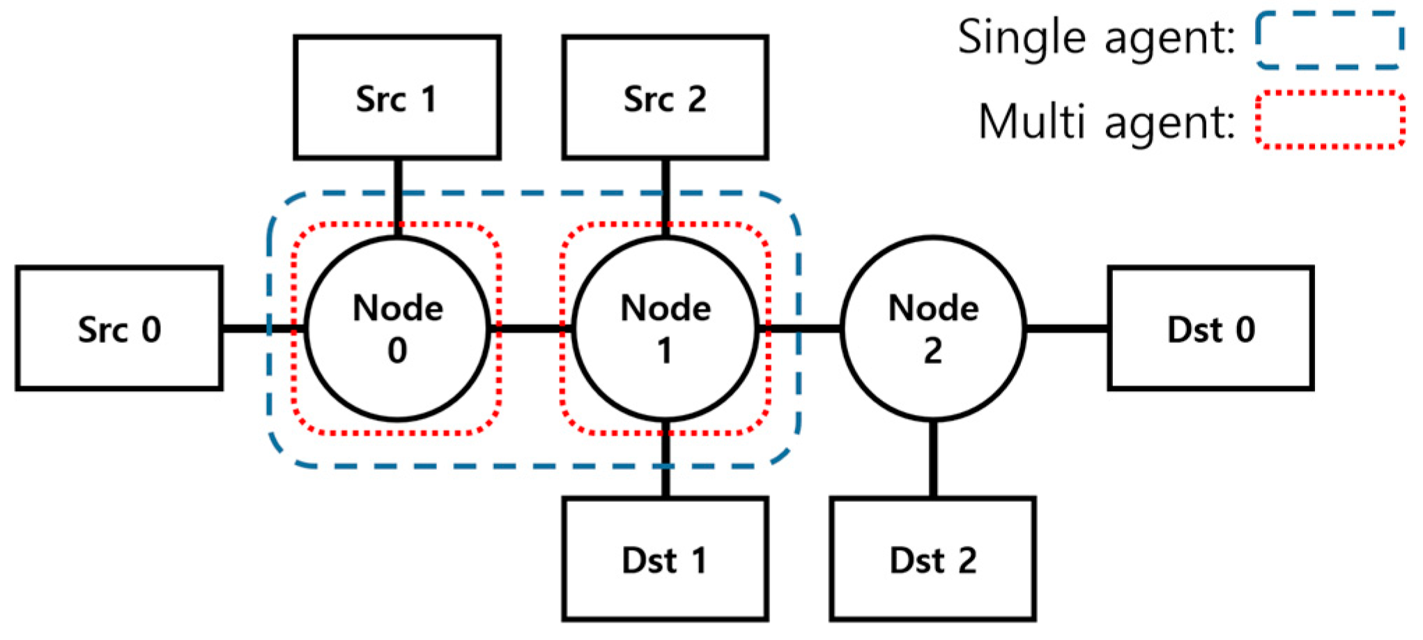
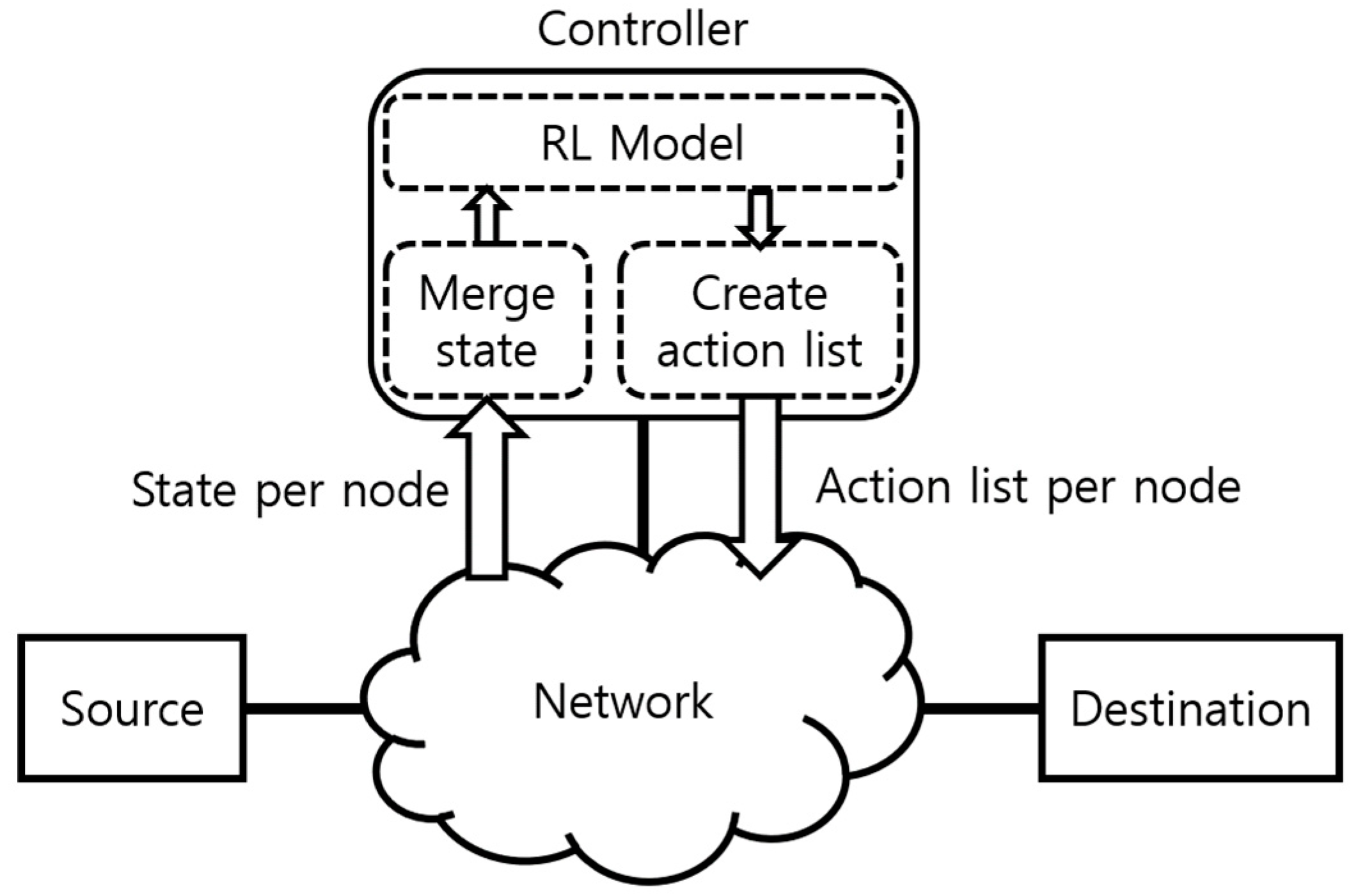
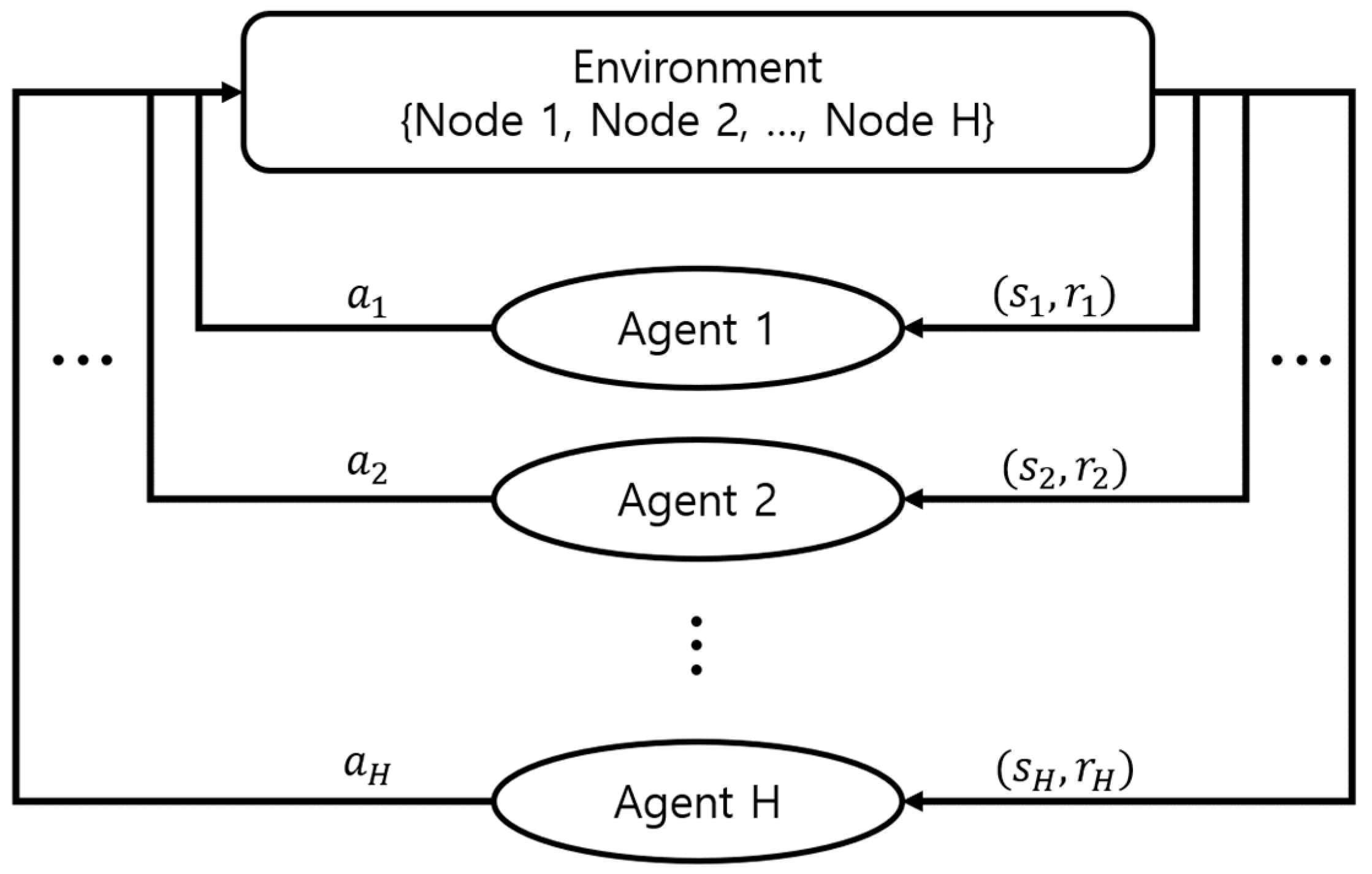
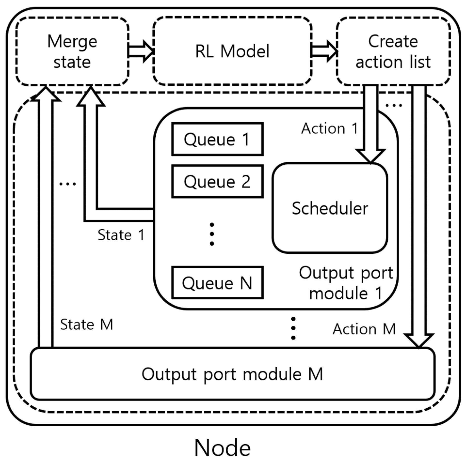
2.3. SARL and MARL
- State
- Action
- Reward
| Algorithm 1. Rewards in a single node. |
| M = number of the output port N = number of the input portOutputPort Module[1..M] OutputPortModule.Queue[1..N] reward = 0 for i in 1..M: if all OutputPortModule[i].Queue is not empty if packet transmission is complete: if all queues are empty: reward += estimated delay of the transmitted packet else: reward += estimated delay of the transmitted packet − max(estimated delay of packets in all queues) else: reward += −max(estimated delay of packets in all queues)2 return reward |
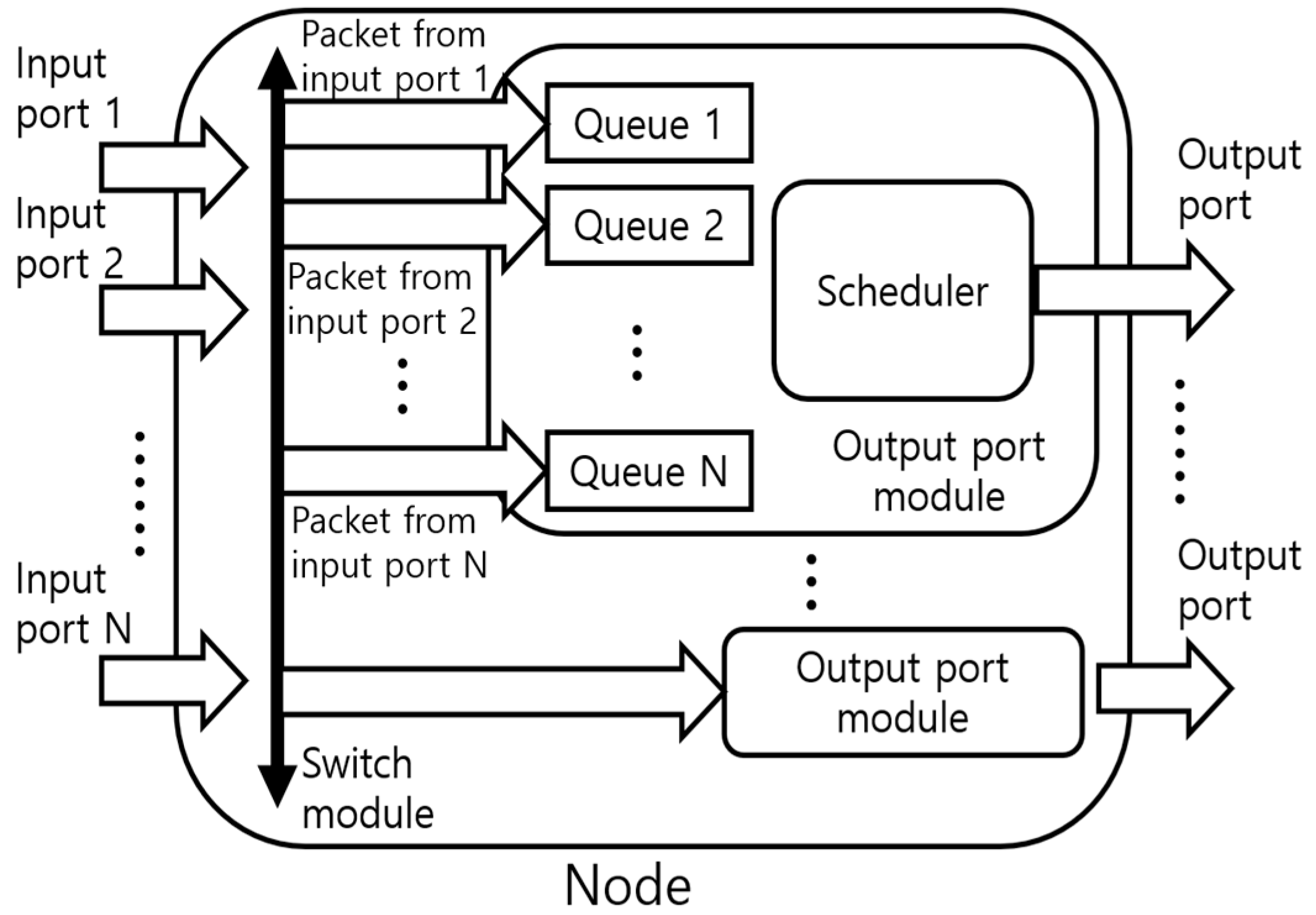
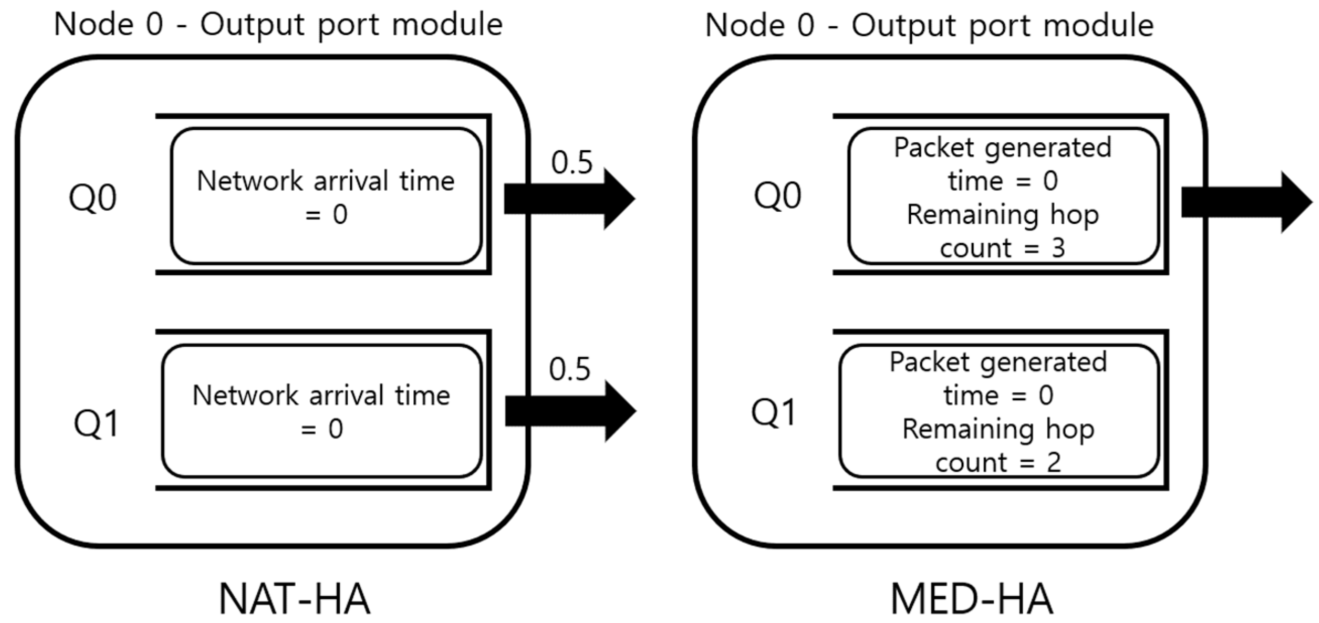
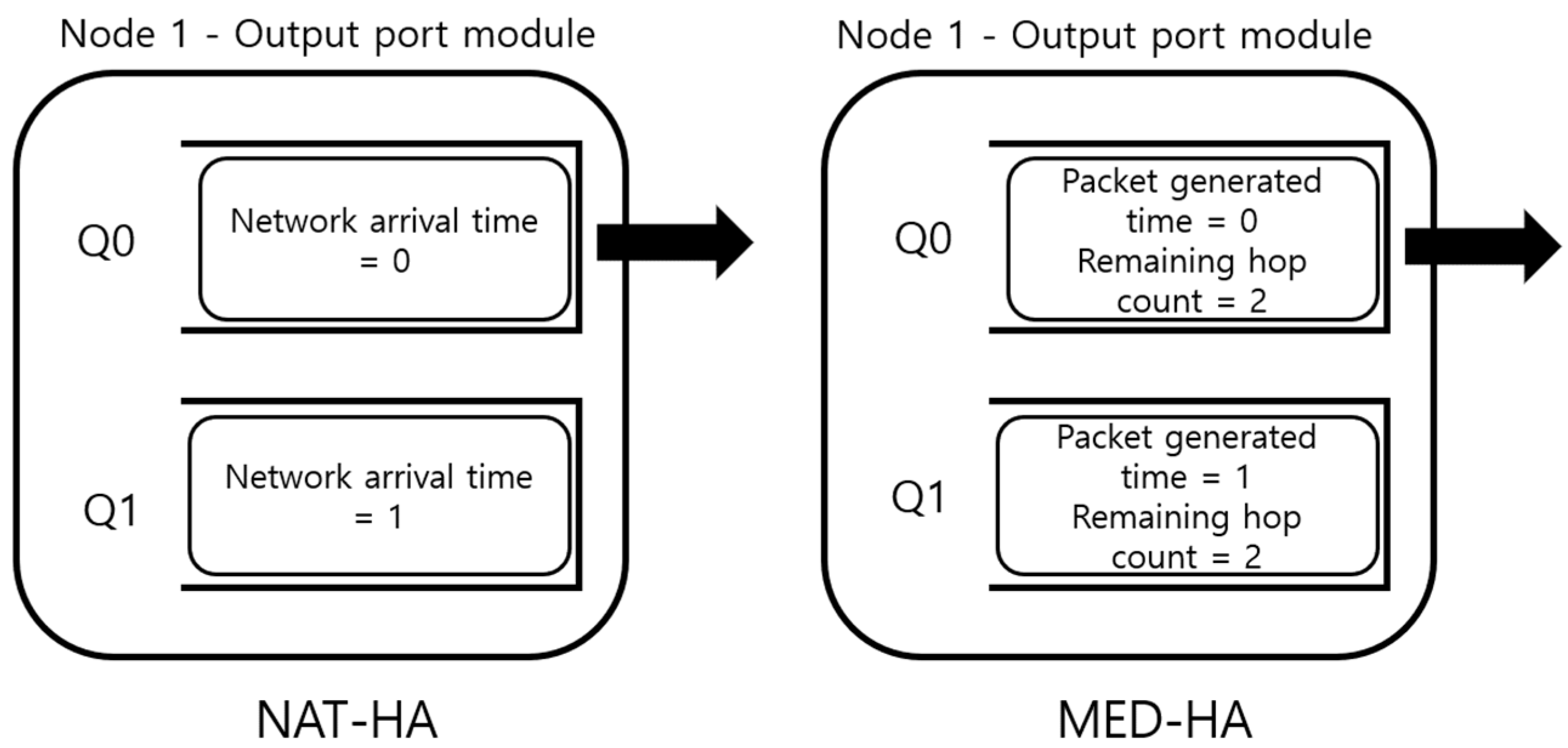
2.4. Scheduler Using Metadata
| Algorithm 2. NAT-HA in the output port module. |
| M = number of the input port Queue[1..M] min_NAT = Inf idx = 0 while true for i in 1..M: if Queue[i] is not empty if min_NAT > Queue[i].head.NAT idx = i min_NAT = Queue[i].head.NAT send(Queue[idx].head) Queue[idx].dequeue |
| Algorithm 3. MED-HA in the output port module. |
| C = link capacity M = number of the input port Queue[1..M] max_estimated_delay = 0 idx = 0 bit_length = 0 while true for i in 1..M: if Queue[i] is not empty for j in 1..Queue[i].length estimated_delay = Queue[i][j].remaining_hop_count × (Queue[i][j].length/C) + time.now − Queue[i][j].generated_time + (bit_length/C) bit_length += Queue[i][j].length if max_estimated_delay < estimated_delay idx = i max_estimated_delay = estimated_delay send(Queue[idx].head) Queue[idx].dequeue |
3. Results
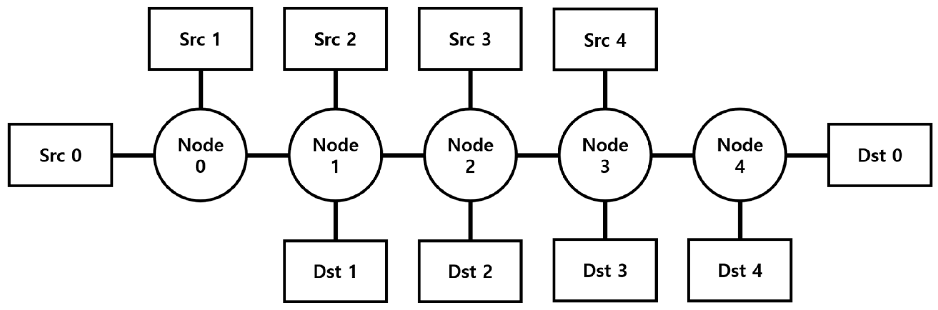
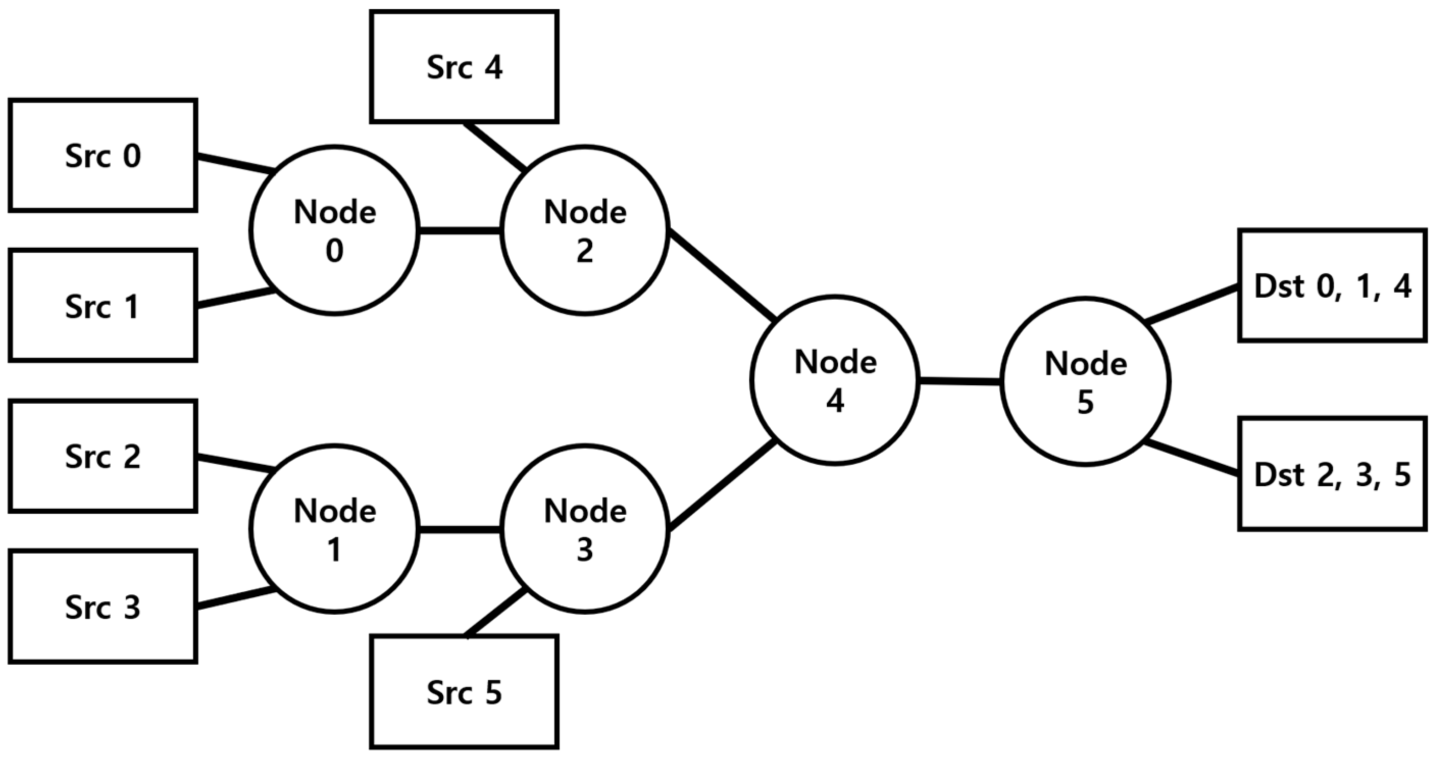
3.1. Simulation Setup
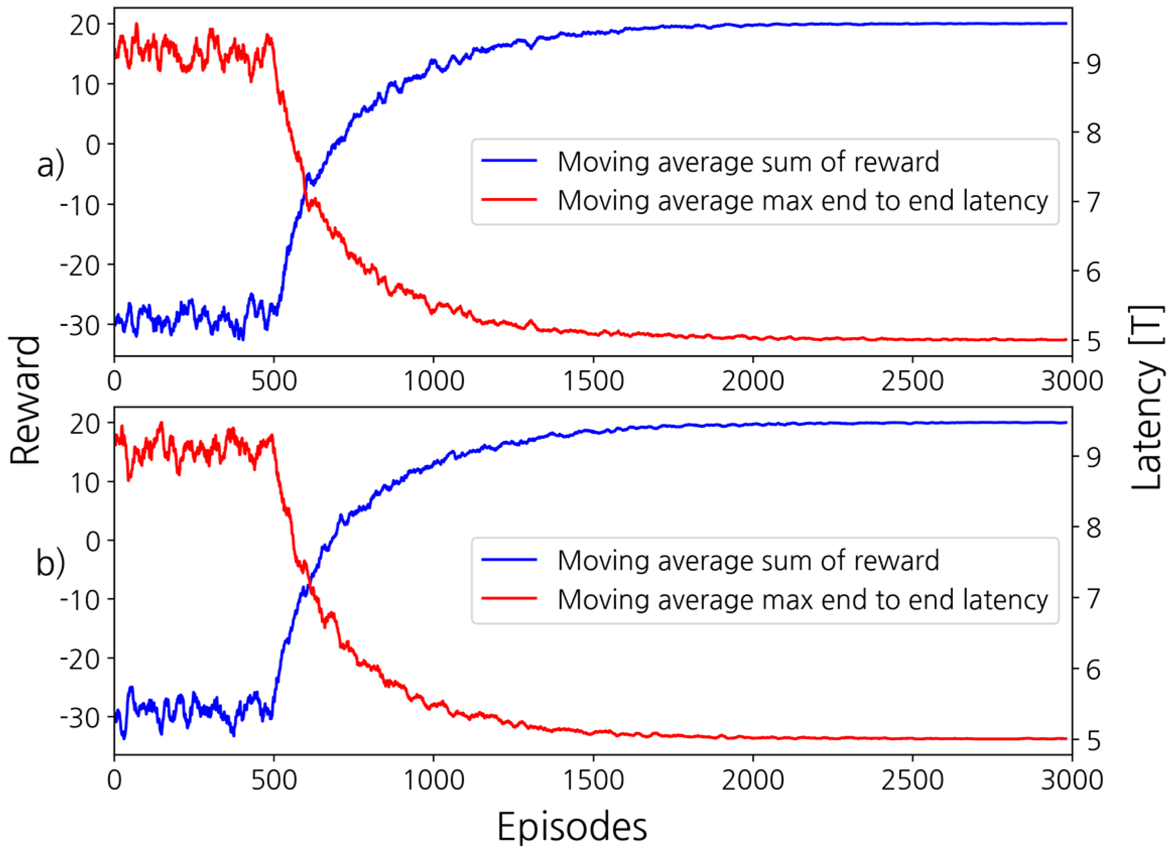
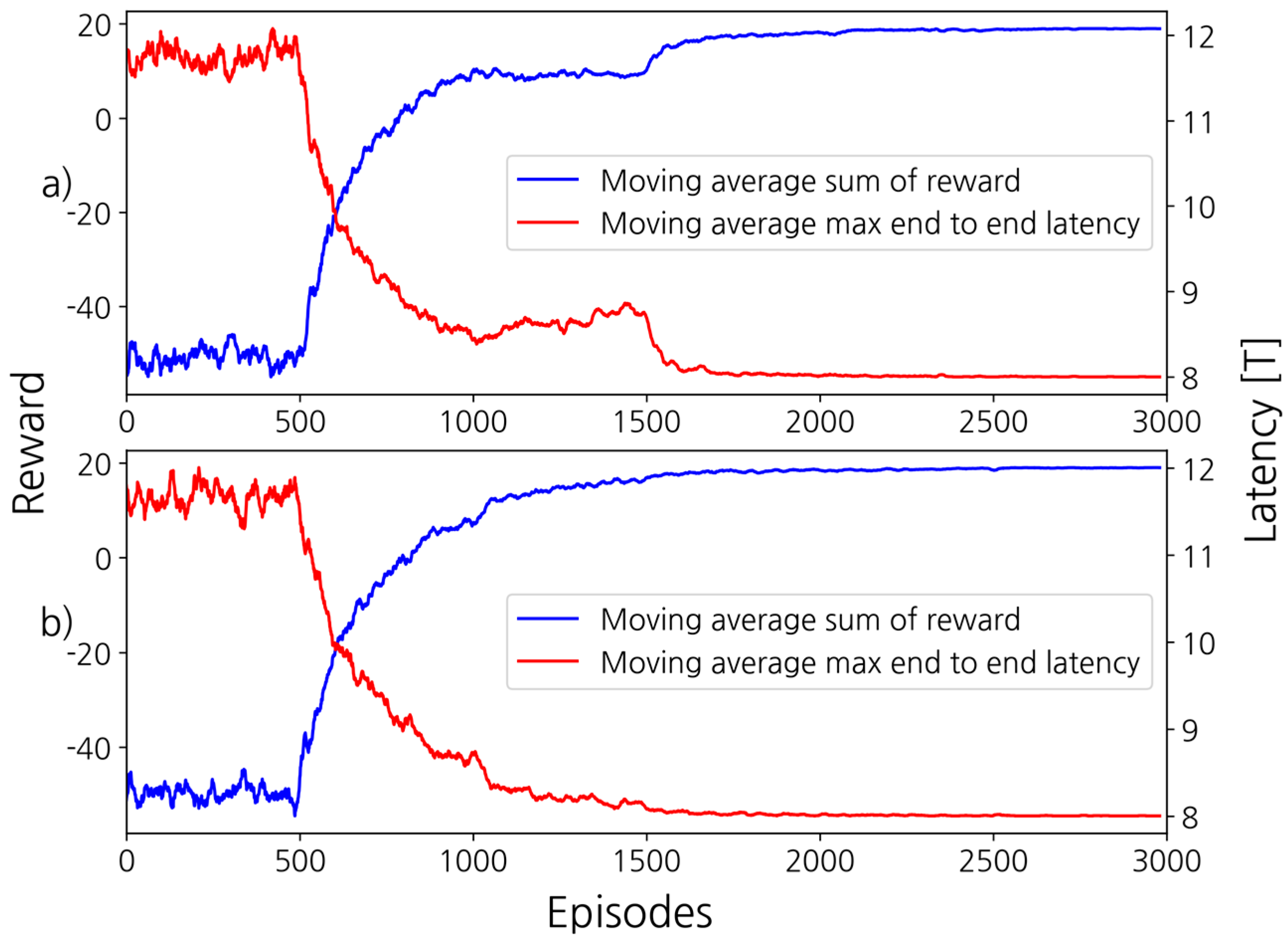
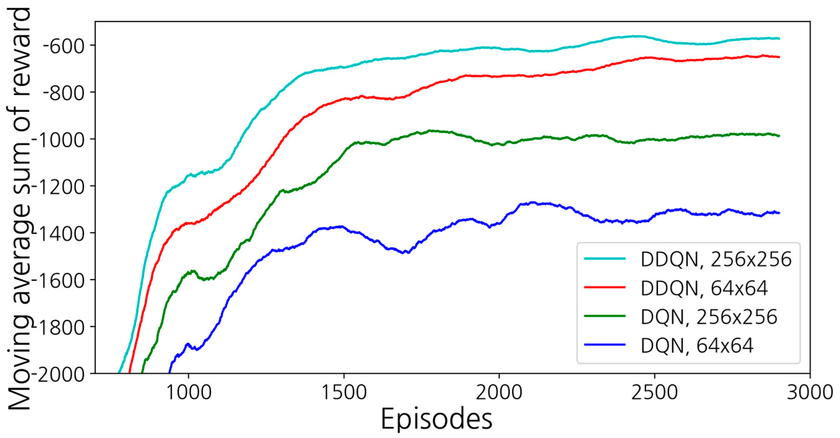
3.2. Simulation
4. Conclusions
Author Contributions
Funding
Institutional Review Board Statement
Informed Consent Statement
Data Availability Statement
Conflicts of Interest
References
- Denda, R.; Banchs, A.; Effelsberg, W. The Fairness Challenge in Computer Networks. In Proceedings of the Quality of Future Internet Services, First COST 263 International Workshop, QofIS 2000, Berlin, Germany, 25–26 September 2000; pp. 208–220. [Google Scholar] [CrossRef] [Green Version]
- Huaizhou, S.H.I.; Prasad, R.V.; Onur, E.; Niemegeers, I.G.M.M. Fairness in Wireless Networks:Issues, Measures and Challenges. IEEE Commun. Surv. Tutor. 2014, 16, 5–24. [Google Scholar] [CrossRef]
- Segment Routing Architecture, IETF RFC 8402, July 2018. Available online: https://datatracker.ietf.org/doc/rfc8402/ (accessed on 17 November 2022).
- Deterministic Networking Architecture, IETF RFC 8655, October 2019. Available online: https://datatracker.ietf.org/doc/rfc8655/ (accessed on 9 August 2022).
- Desmouceaux, Y.; Pfister, P.; Tollet, J.; Townsley, M.; Clausen, T. 6LB: Scalable and Application-Aware Load Balancing with Segment Routing. IEEE/ACM Trans. Netw. 2018, 26, 819–834. [Google Scholar] [CrossRef]
- Joung, J.; Kwon, J. Zero Jitter for Deterministic Networks Without Time-Synchronization. IEEE Access 2021, 9, 49398–49414. [Google Scholar] [CrossRef]
- Deterministic Networking (DetNet) Data Plane Framework, IETF RFC 8938, November 2020. Available online: https://www.rfc-editor.org/rfc/rfc8938 (accessed on 12 August 2022).
- Wang, P.; Ma, S.; Hongyi, L.; Wang, Z.; Chen, L. Adaptive Remaining Hop Count Flow Control: Consider the Interaction between Packets. In Proceedings of the 20th Asia and South Pacific Design Automation Conference, Chiba, Japan, 19–22 January 2015; 22 January 2015. [Google Scholar] [CrossRef]
- Alizadeh, M.; Yang, S.; Sharif, M.; Katti, S.; McKeown, N.; Prabhakar, B.; Shenker, S. pFabric. In Proceedings of the ACM SIGCOMM 2013 Conference on SIGCOMM, Hong Kong, China, 12–16 August 2013. [Google Scholar] [CrossRef]
- Sharma, N.K.; Zhao, C.; Liu, M.; Kannan, P.G.; Kim, C.; Krishnamurthy, A.; Sivaraman, A. Programmable calendar queues for high-speed packet scheduling. In Proceedings of the 17th USENIX Symposium on Networked Systems Design and Implementation (NSDI 20), Santa Clara, CA, USA, 25–27 February 2020; pp. 685–699. [Google Scholar]
- Yu, Z.; Hu, C.; Wu, J.; Sun, X.; Braverman, V.; Chowdhury, M.; Liu, Z.; Jin, X. Programmable Packet Scheduling with a Single Queue. In Proceedings of the 2021 ACM SIGCOMM 2021 Conference, Virtual, 23–27 August 2021. [Google Scholar] [CrossRef]
- Shrivastav, V. Fast, Scalable, and Programmable Packet Scheduler in Hardware. In Proceedings of the ACM Special Interest Group on Data Communication, Beijing, China, 19–23 August 2019. [Google Scholar] [CrossRef]
- Kolhar, M. Using the Packet Header Redundant Fields to Improve VoIP Bandwidth Utilization. Electr. Electron. Eng. 2021, Preprints. [Google Scholar] [CrossRef]
- Dinda, P.A. Exploiting packet header redundancy for zero cost dissemination of dynamic resource information. In Proceedings of the 6th Workshop on Languages, Compilers, and Run-Time Systems for Scalable Computer (LCR 2002), Washington, DC, USA, 1 May 2002. [Google Scholar]
- Chen, J.; Wang, Y.; Lan, T. Bringing Fairness to Actor-Critic Reinforcement Learning for Network Utility Optimization. In Proceedings of the IEEE INFOCOM 2021–IEEE Conference on Computer Communications, Vancouver, BC, Canada, 10–13 May 2021. [Google Scholar] [CrossRef]
- López-Sánchez, M.; Villena-Rodríguez, A.; Gómez, G.; Martín-Vega, F.J.; Aguayo-Torres, M.C. Latency Fairness Optimization on Wireless Networks through Deep Reinforcement Learning. arXiv 2022, arXiv:2201.10281. [Google Scholar] [CrossRef]
- Jiang, J.; Lu, Z. Learning fairness in multi-agent systems. In Proceedings of the Advances in Neural Information Processing Systems 32: Annual Conference on Neural Information Processing Systems 2019, Vancouver, BC, Canada, 8–14 December 2019. [Google Scholar]
- Nguyen, C.T.; Van Huynh, N.; Chu, N.H.; Saputra, Y.M.; Hoang, D.T.; Nguyen, D.N.; Pham, Q.-V.; Niyato, D.; Dutkiewicz, E.; Hwang, W.-J. Transfer Learning for Future Wireless Networks: A Comprehensive Survey. arXiv 2021, arXiv:2102.07572. [Google Scholar]
- Cheng, Y.; Yin, B.; Zhang, S. Deep Learning for Wireless Networking: The Next Frontier. IEEE Wirel. Commun. 2021, 28, 176–183. [Google Scholar] [CrossRef]
- Kim, D.; Lee, T.; Kim, S.; Lee, B.; Youn, H.Y. Adaptive Packet Scheduling in IoT Environment Based on Q-Learning. Procedia Comput. Sci. 2018, 141, 247–254. [Google Scholar] [CrossRef]
- Guo, B.; Zhang, X.; Wang, Y.; Yang, H. Deep-Q-Network-Based Multimedia Multi-Service QoS Optimization for Mobile Edge Computing Systems. IEEE Access 2019, 7, 160961–160972. [Google Scholar] [CrossRef]
- Marchang, J.; Ghita, B.; Lancaster, D. Hop-Based Dynamic Fair Scheduler for Wireless Ad-Hoc Networks. In Proceedings of the 2013 IEEE International Conference on Advanced Networks and Telecommunications Systems (ANTS), Kattankulathur, India, 15–18 December 2013. [Google Scholar] [CrossRef]
- Lee, E.M.; Kashif, A.; Lee, D.H.; Kim, I.T.; Park, M.S. Location based multi-queue scheduler in wireless sensor network. In Proceedings of the 2010 the 12th International Conference on Advanced Communication Technology (ICACT), Gangwon-Do, Republic of Korea, 7–10 February 2010; pp. 551–555. [Google Scholar]
- Peng, Y.; Liu, Q.; Varman, P. Latency Fairness Scheduling for Shared Storage Systems. In Proceedings of the 2019 IEEE International Conference on Networking, Architecture and Storage (NAS), Enshi, China, 15–17 August 2019. [Google Scholar] [CrossRef]
- Watkins, C.J.C.H.; Dayan, P. Q-Learning. Mach. Learn. 1992, 8, 279–292. [Google Scholar] [CrossRef]
- Mnih, V.; Kavukcuoglu, K.; Silver, D.; Graves, A.; Antonoglou, I.; Wierstra, D.; Riedmiller, M. Playing Atari with Deep Reinforcement Learning. arXiv 2013, arXiv:1312.5602. [Google Scholar]
- Van Hasselt, H.; Guez, A.; Silver, D. Deep Reinforcement Learning with Double Q-Learning. In Proceedings of the AAAI Conference on Artificial Intelligence, Phoenix, AZ, USA, 12–17 February 2016. [Google Scholar] [CrossRef]
- Hasselt, H. Double Q-learning. In Proceedings of the Advances in Neural Information Processing Systems 23: 24th Annual Conference on Neural Information Processing Systems 2010, Vancouver, BC, Canada, 6–9 December 2010. [Google Scholar]
- Schaul, T.; Quan, J.; Antonoglou, I.; Silver, D. Prioritized Experience Replay. arXiv 2015, arXiv:1511.05952. [Google Scholar]
- Tan, M. Multi-agent reinforcement learning: Independent vs. cooperative agents. In Proceedings of the Tenth International Conference on Machine Learning, Amherst, MA, USA, 27–29 July 1993; pp. 330–337. [Google Scholar]
- Time-Sensitive Networking Task Group. IEEE802.org. Available online: https://www.ieee802.org/1/pages/tsn.html (accessed on 23 August 2022).
- Jain, R.; Chiu, D.; Hawe, W. A Quantitative Measure of Fairness and Discrimination For Resource Allocation in Shared Computer Systems. arXiv 1998, arXiv:cs/9809099. [Google Scholar]
- TensorFlow. Available online: https://www.tensorflow.org/?hl=ko (accessed on 13 May 2022).
- Joung, J.; Kwon, J.; Ryoo, J.-D.; Cheung, T. Asynchronous Deterministic Network Based on the DiffServ Architecture. IEEE Access 2022, 10, 15068–15083. [Google Scholar] [CrossRef]


| Symbol | Meaning |
|---|---|
| Q | Q-table or deep learning network |
| S, s | State |
| A, a | Action |
| R, r | Reward |
| T | Time |
| α | Learning rate |
| Discount factor | |
| θ | Deep learning network’s weights |
| Y | Target Q-value |
| Symbol | Meaning |
|---|---|
| M | Number of an output port |
| N | Number of an input port |
| H | Number of nodes |
| C | Link capacity |
| T | Unit time in simulation |
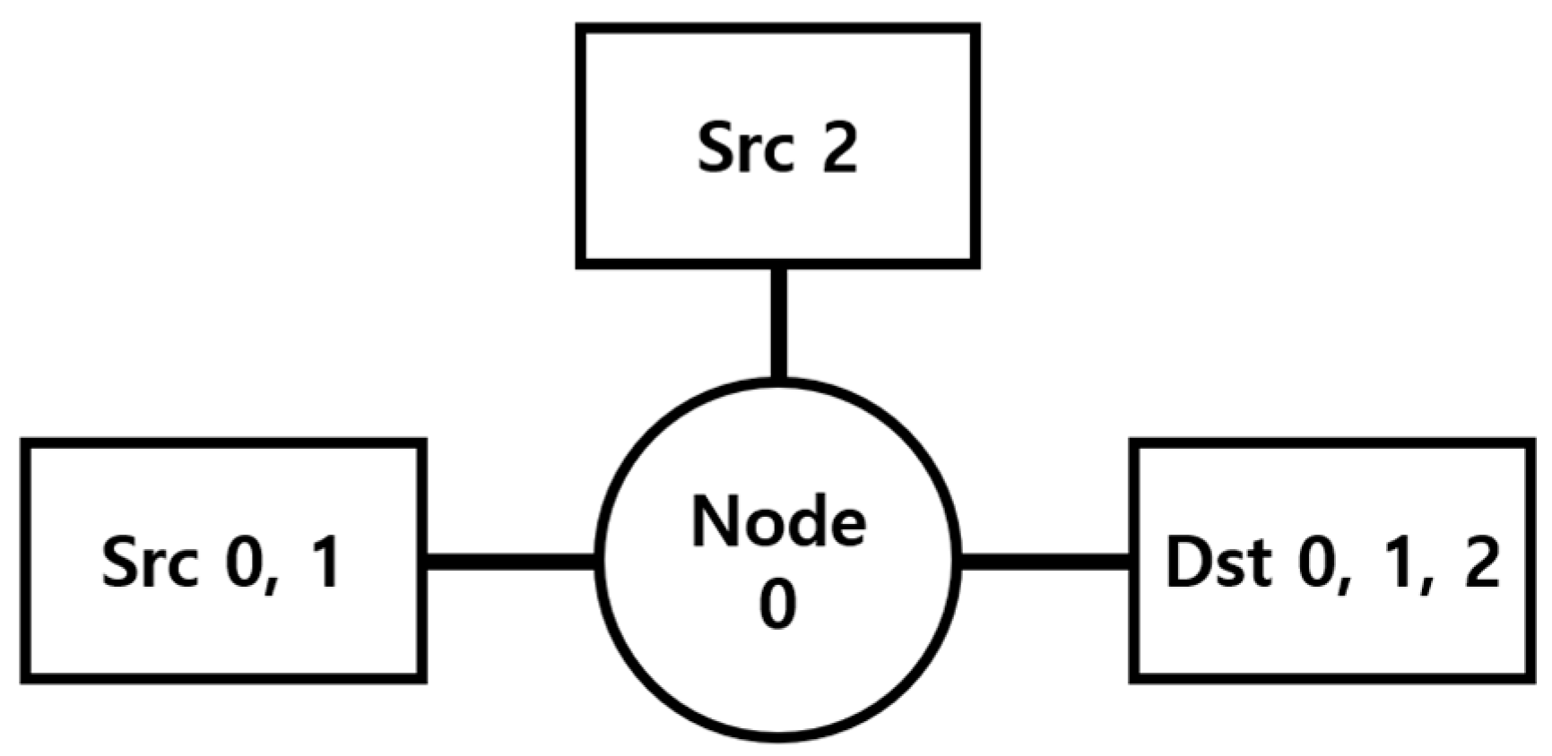
| Time | Source 0 | Source 1 | Source 2 |
|---|---|---|---|
| 0 | 1 | 1 | |
| T | 1 |
| Type | Size |
|---|---|
| Input | The state size |
| Dense | 64 |
| ReLu | 64 |
| Dense | 64 |
| ReLu | 64 |
| Dense(Output) | 1 |
| Hyperparameter | Value |
|---|---|
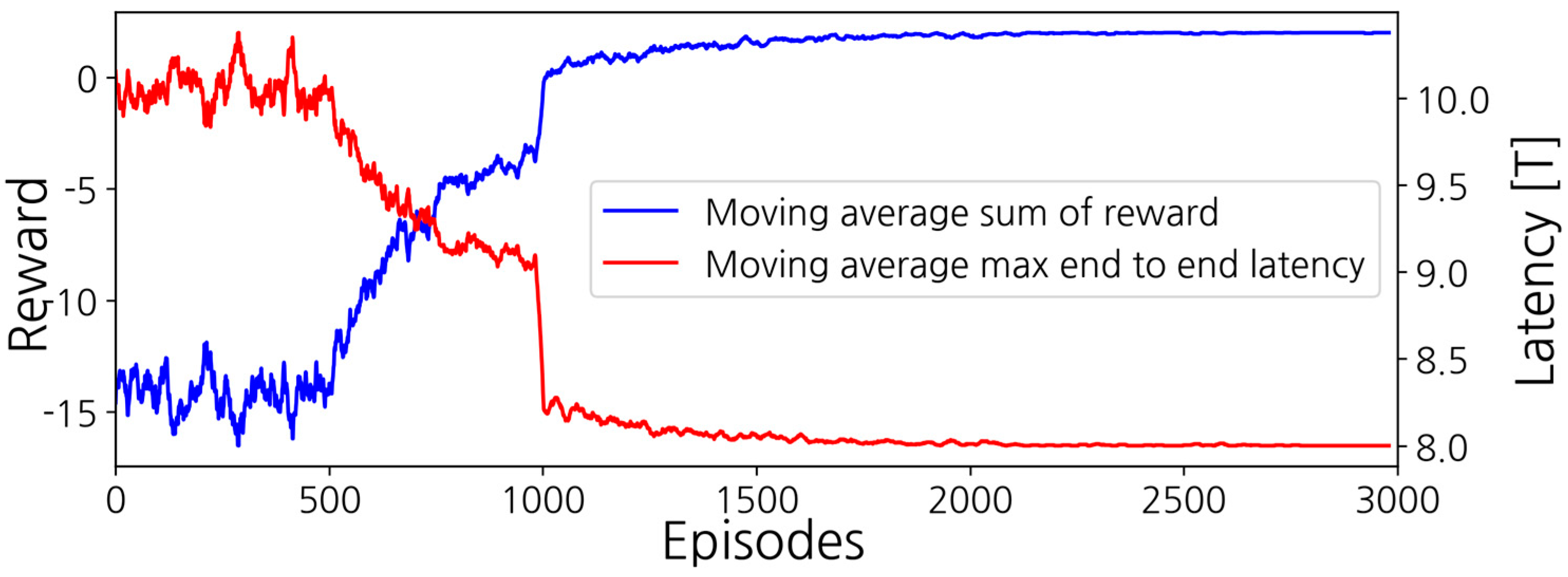
| Number of episodes | 3000 |
| Initial learning rate () | 0.002 |
| Discount factor | 0.99 |
| Initial epsilon | 1 |
| Epsilon decay | 0.997 |
| Minimum epsilon | 0.001 |
| Target model update cycle | 500 episodes |
| Batch size | 256 |
| Learning rate decay period (d) | 2500 episodes |
| Time | Source 0 | Source 1 | Source 2 | Source 3 | Source 4 |
|---|---|---|---|---|---|
| 0 | 1 | 1 | |||
| T | 1 | ||||
| 2T | 1 | ||||
| 3T | 1 |
| Time | Source 0 | Source 1 | Source 2 | Source 3 | Source 4 | Source 5 |
|---|---|---|---|---|---|---|
| 0 | 1 | 1 | 1 | 1 | ||
| T | 1 | 1 |
| Time | Source 0 | Source 1 | Source 2 |
|---|---|---|---|
| 0 | 1 | 1 | |
| T | 1 |
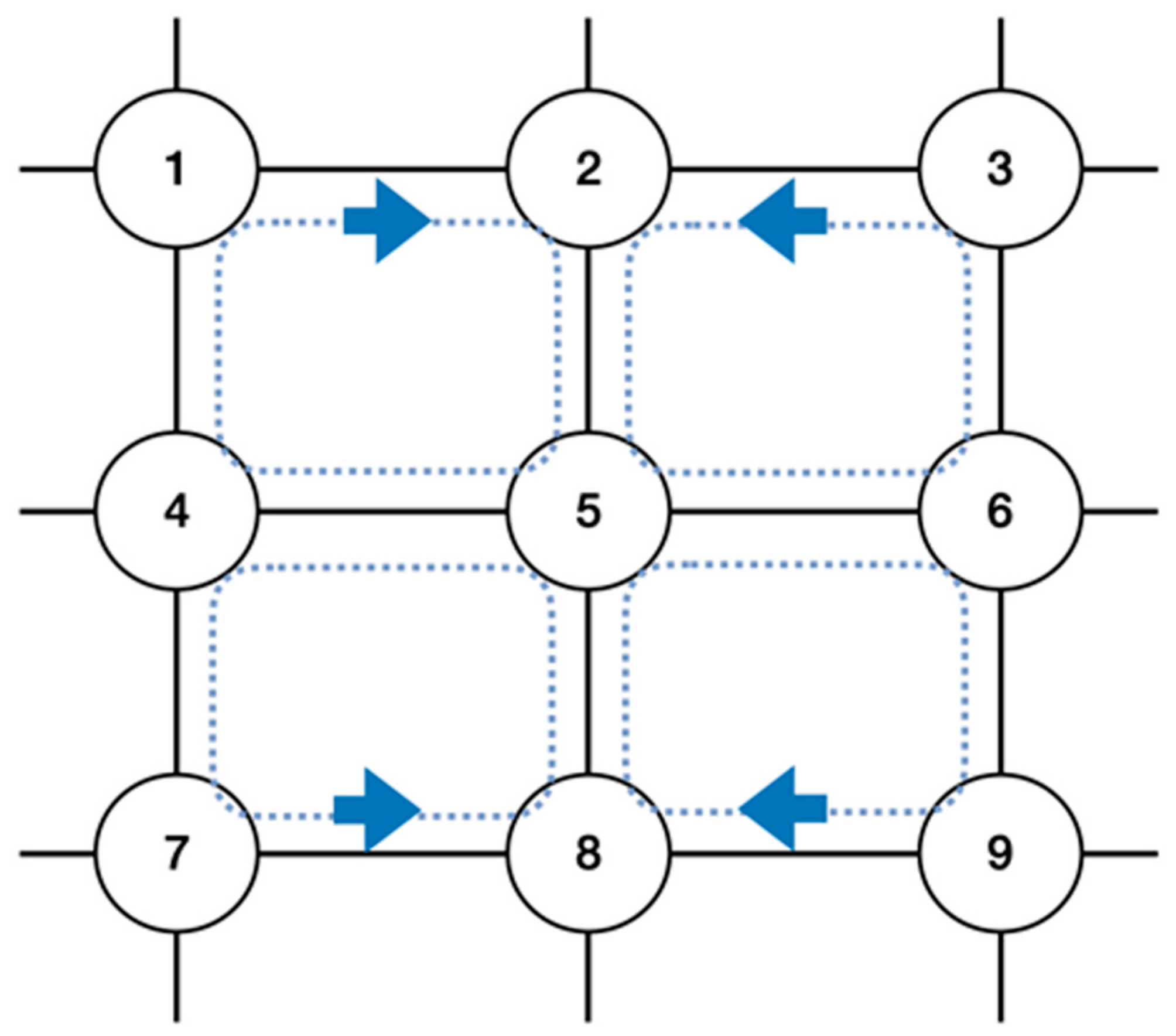
| Flow Number | Route |
|---|---|
| 0 | 1-2-5-6-9 |
| 1 | 4-1-2 |
| 2 | 4-7-8 |
| 3 | 7-8-5-6-3 |
| 4 | 3-2-5-4-7 |
| 5 | 6-3-2 |
| 6 | 6-9-8 |
| 7 | 9-8-5-4-1 |
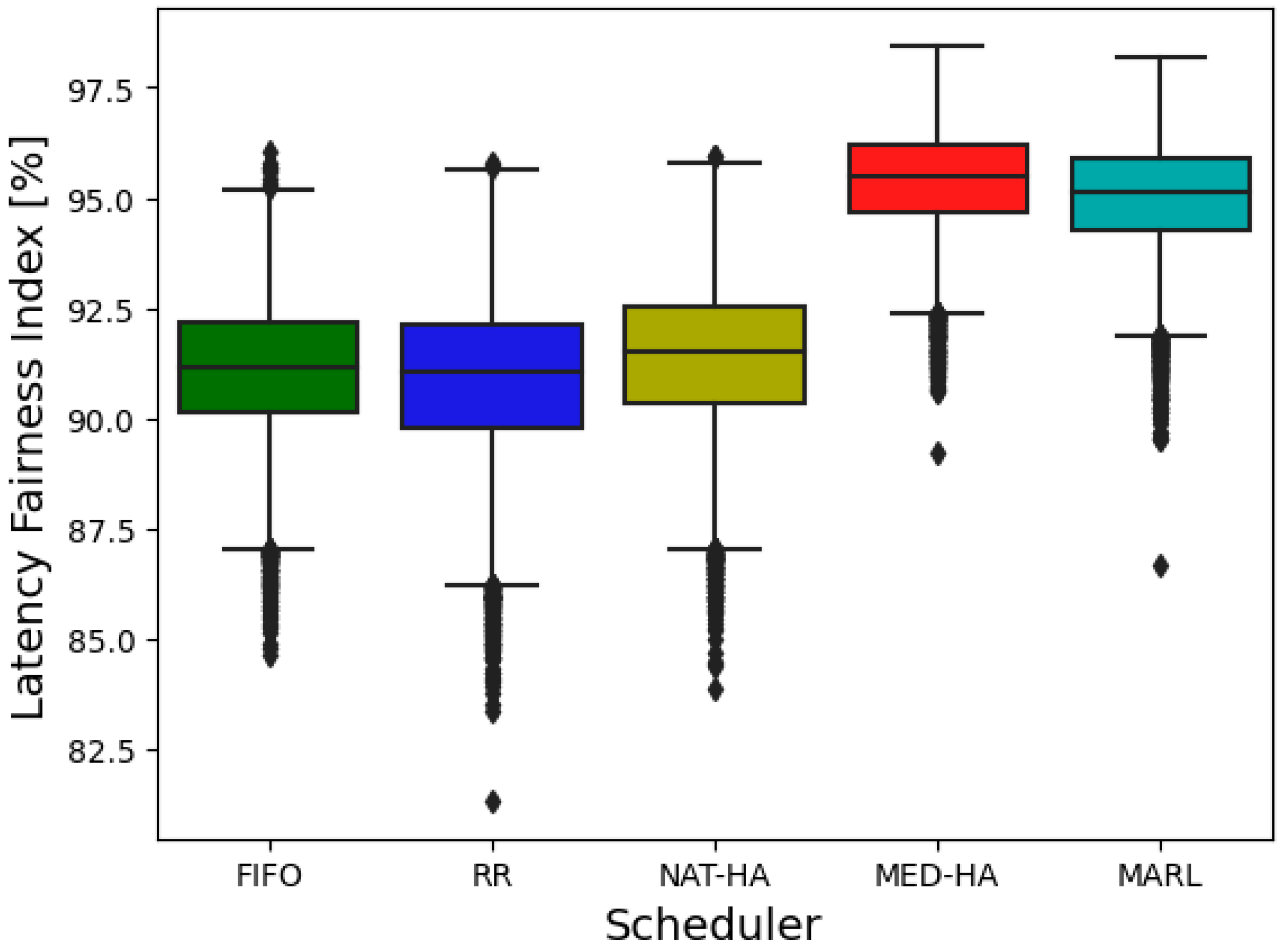
| Latency Fairness Index [%] | |||||
|---|---|---|---|---|---|
| FIFO | RR | NAT-HA | MED-HA | MARL | |
| Mean | 91.1 | 90.89 | 91.38 | 95.39 | 95.01 |
| Min | 84.62 | 81.33 | 84 | 89.2 | 96.65 |
| Max | 96.07 | 95.78 | 96.01 | 98.44 | 98.18 |
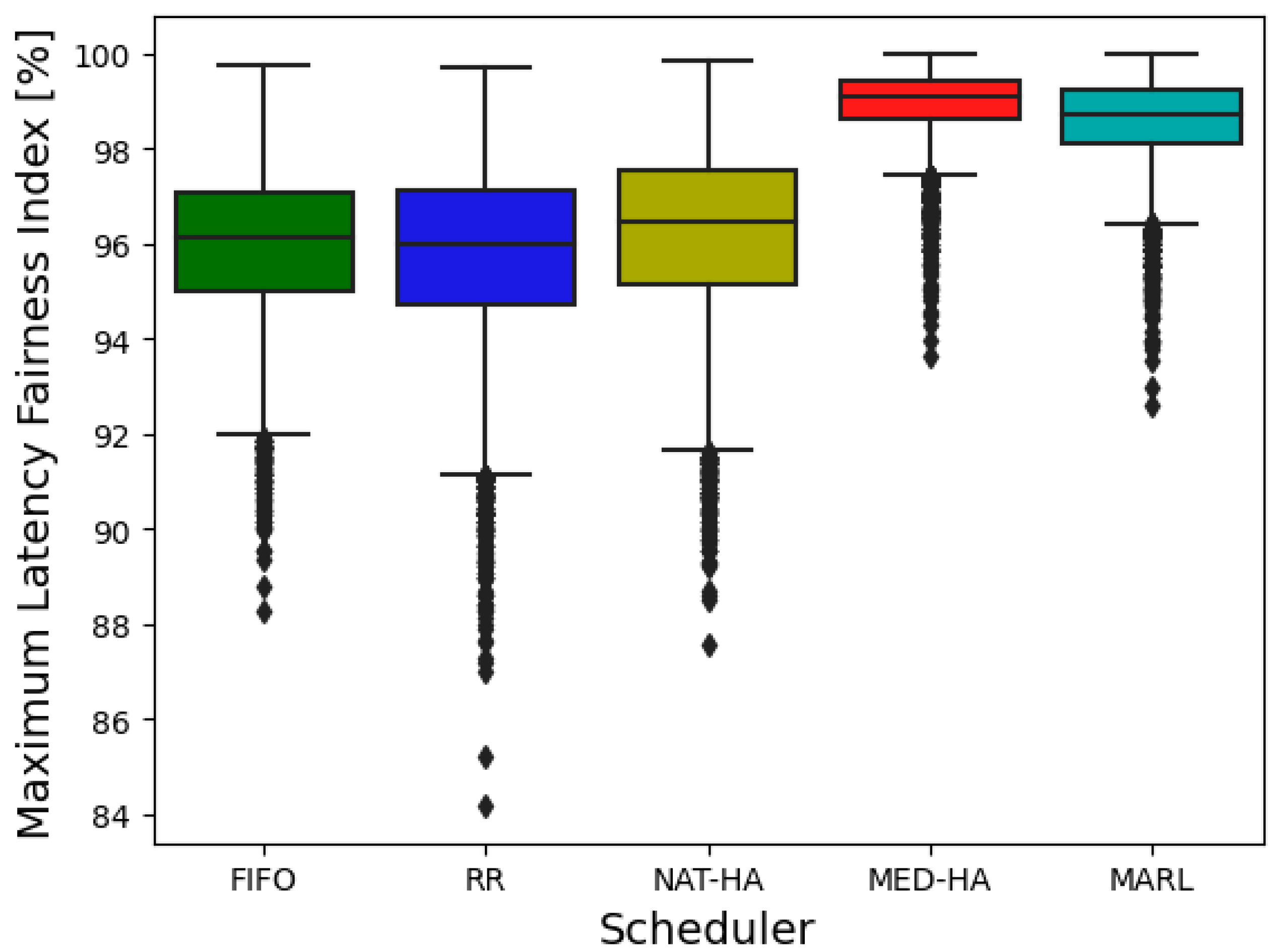
| Maximum Latency Fairness Index [%] | |||||
|---|---|---|---|---|---|
| FIFO | RR | NAT-HA | MED-HA | MARL | |
| Mean | 95.96 | 95.79 | 96.22 | 98.91 | 98.57 |
| Min | 88.28 | 84.18 | 87.55 | 93.64 | 92.6 |
| Max | 99.78 | 99.73 | 99.82 | 100 | 100 |
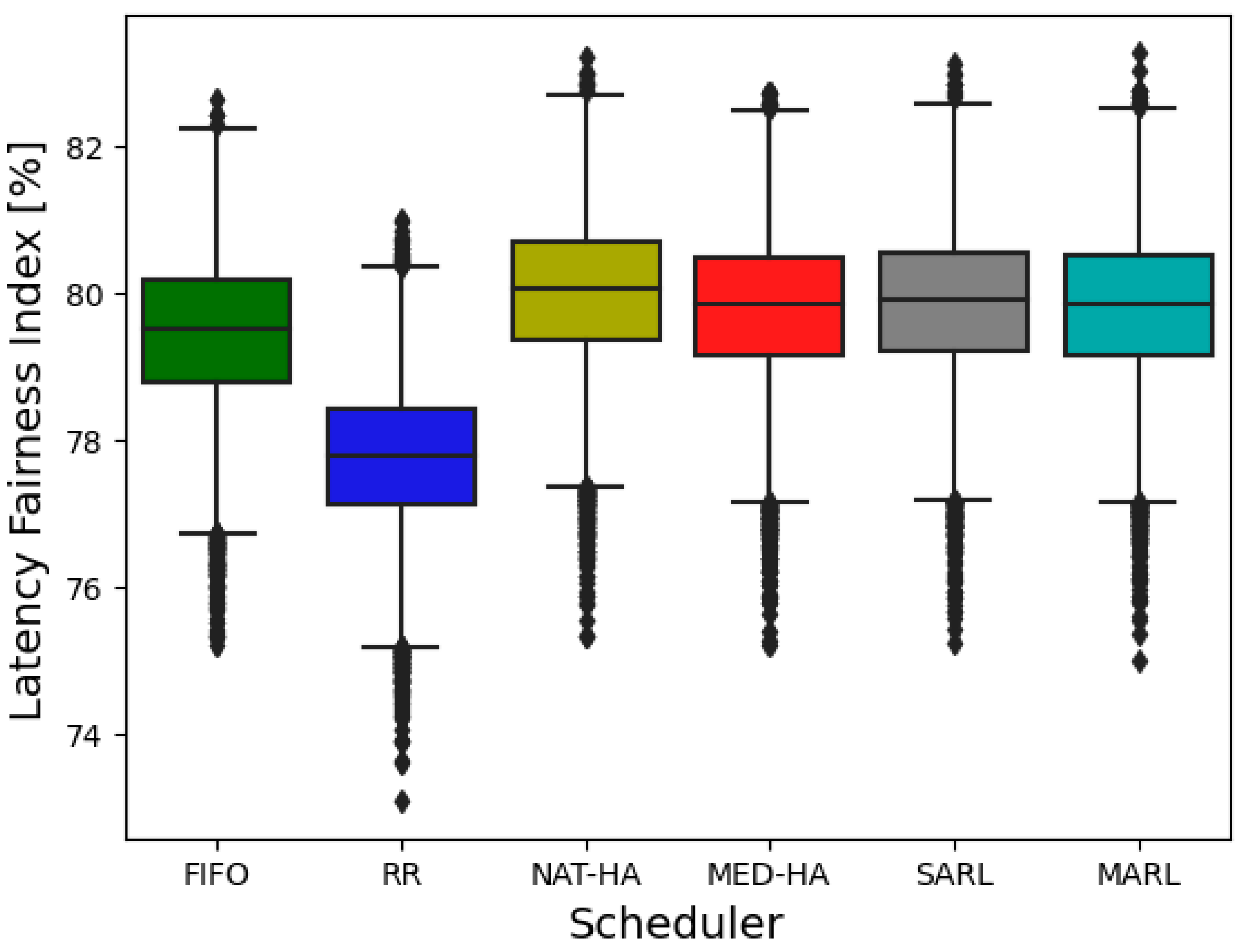
| Latency Fairness Index [%] | ||||||
|---|---|---|---|---|---|---|
| FIFO | RR | NAT-HA | MED-HA | SARL | MARL | |
| Mean | 79.46 | 77.75 | 80 | 79.8 | 79.85 | 79.81 |
| Min | 75.21 | 73.1 | 75.33 | 75.22 | 75.24 | 75 |
| Max | 82.62 | 81.01 | 83.21 | 82.73 | 83.13 | 83.28 |
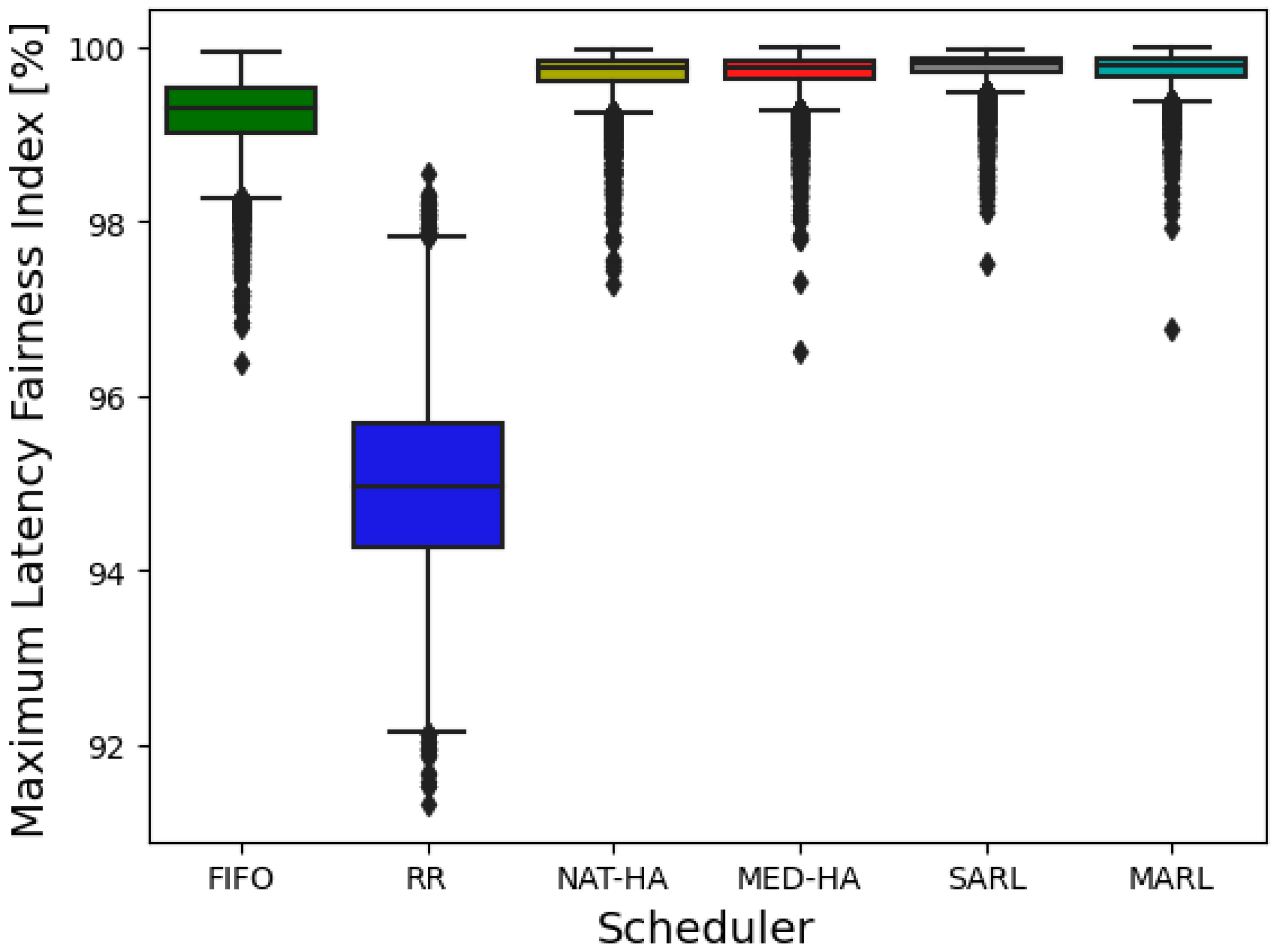
| Maximum Latency Fairness Index [%] | ||||||
| FIFO | RR | NAT-HA | MED-HA | SARL | MARL | |
| Mean | 99.22 | 94.99 | 99.68 | 99.7 | 99.77 | 99.74 |
| Min | 96.38 | 91.33 | 96.49 | 96.5 | 97.51 | 96.76 |
| Max | 99.93 | 98.54 | 99.98 | 99.99 | 99.97 | 99.99 |
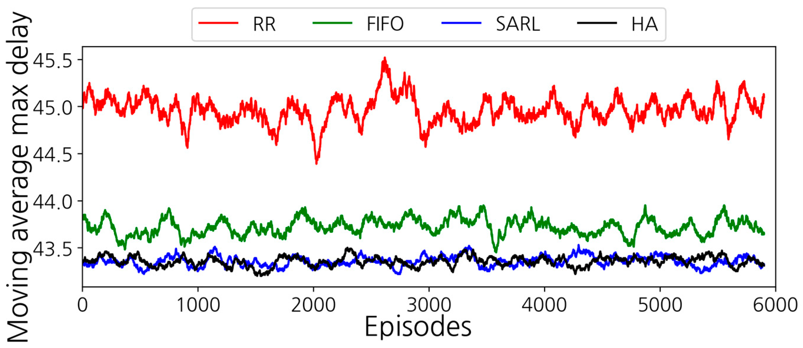
| Topology | Average Maximum E2E Latency | |||||
|---|---|---|---|---|---|---|
| FIFO | RR | NAT-HA | MED-HA | SARL | MARL | |
| 1 | 5.9375T | 5.9375T | 5.5T | 5T | 5T | 5T |
| 2 | 9T | 9T | 8T | 8T | 8T | 8T |
| 3 | 9T | 9T | 9T | 9T | 8T | 8T |
| 2 with random flow | 43.711T | 44.13T | 43.281T | 43.27T | 43.279T | 43.274T |
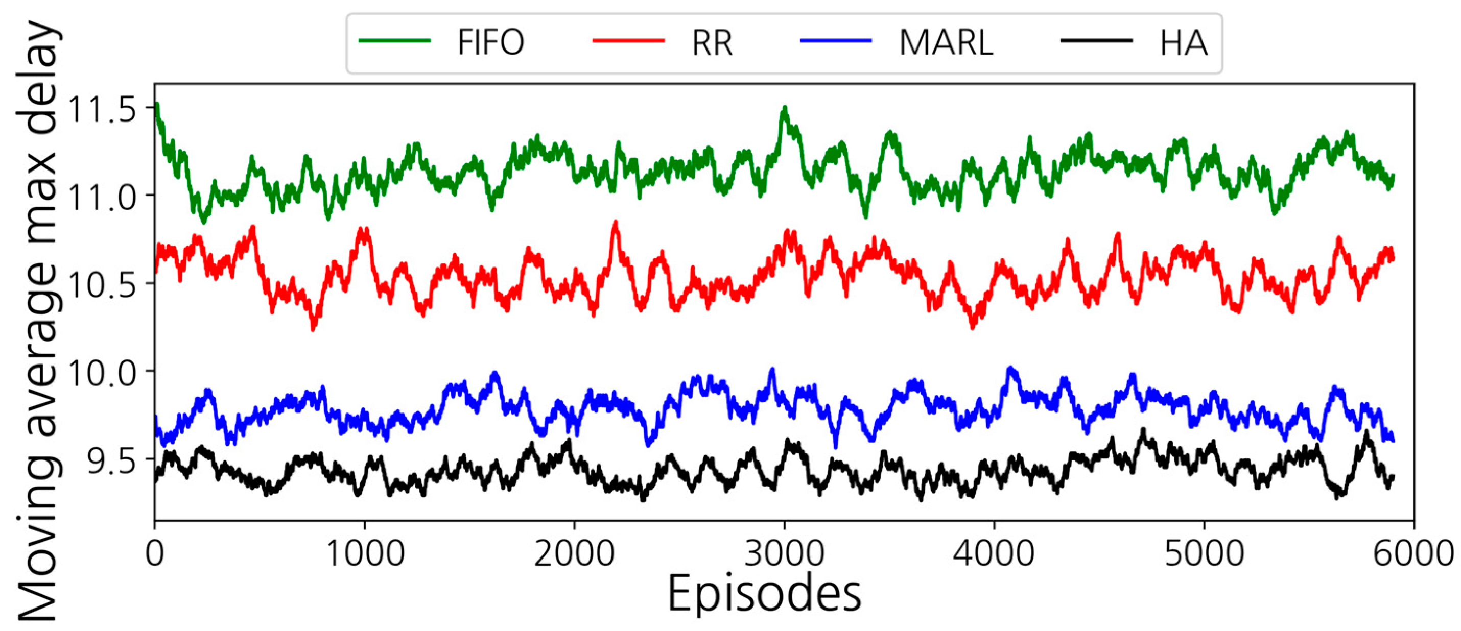
| 4 with random flow | 11.134T | 10.481T | 10.173T | 9.433T | 9.423T | |
Disclaimer/Publisher’s Note: The statements, opinions and data contained in all publications are solely those of the individual author(s) and contributor(s) and not of MDPI and/or the editor(s). MDPI and/or the editor(s) disclaim responsibility for any injury to people or property resulting from any ideas, methods, instructions or products referred to in the content. |
© 2023 by the authors. Licensee MDPI, Basel, Switzerland. This article is an open access article distributed under the terms and conditions of the Creative Commons Attribution (CC BY) license (https://creativecommons.org/licenses/by/4.0/).
Share and Cite
Kwon, J.; Ryu, J.; Lee, J.H.; Joung, J. Improving End-To-End Latency Fairness Using a Reinforcement-Learning-Based Network Scheduler. Appl. Sci. 2023, 13, 3397. https://doi.org/10.3390/app13063397
Kwon J, Ryu J, Lee JH, Joung J. Improving End-To-End Latency Fairness Using a Reinforcement-Learning-Based Network Scheduler. Applied Sciences. 2023; 13(6):3397. https://doi.org/10.3390/app13063397
Chicago/Turabian StyleKwon, Juhyeok, Jihye Ryu, Jee Hang Lee, and Jinoo Joung. 2023. "Improving End-To-End Latency Fairness Using a Reinforcement-Learning-Based Network Scheduler" Applied Sciences 13, no. 6: 3397. https://doi.org/10.3390/app13063397