
Data-Quality Assessment for Digital Twins Targeting Multi-Component Degradation in Industrial Internet of Things (IIoT)-Enabled Smart Infrastructure Systems


Abstract
:Featured Application
Abstract
1. Introduction
- Definition of a measurement system analysis process for developing fault detection and isolation algorithms for multi-component degradation;
- Investigation of the impact of data quality on the development of fault detection and isolation algorithms for multi-component degradation for IIoT-enabled smart infrastructure systems;
- Delineation of an application development process with clear steps for the quantification of data quality before it is used for the design and development of services for IIoT-enabled water distribution systems;
- Demonstration of a practical implementation of the application of a measurement system assessment and offering of perspectives on the impact of data quality on SPC applications, an ensemble model of ML techniques, and neural networks, which can act as a reference for data analysts operating in the DT/IIoT space.
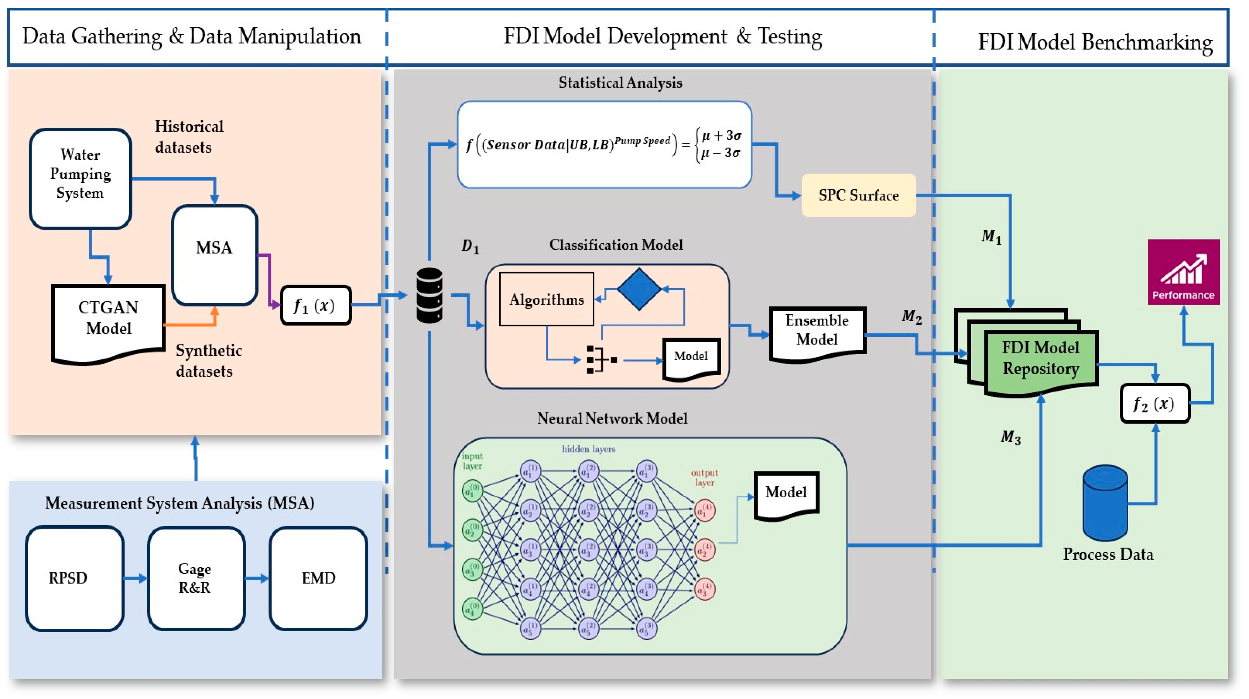
2. Methodology
2.1. Methodology for the Assessment of Data Quality
2.1.1. Measurement System Analysis (MSA)—Methodology Overview
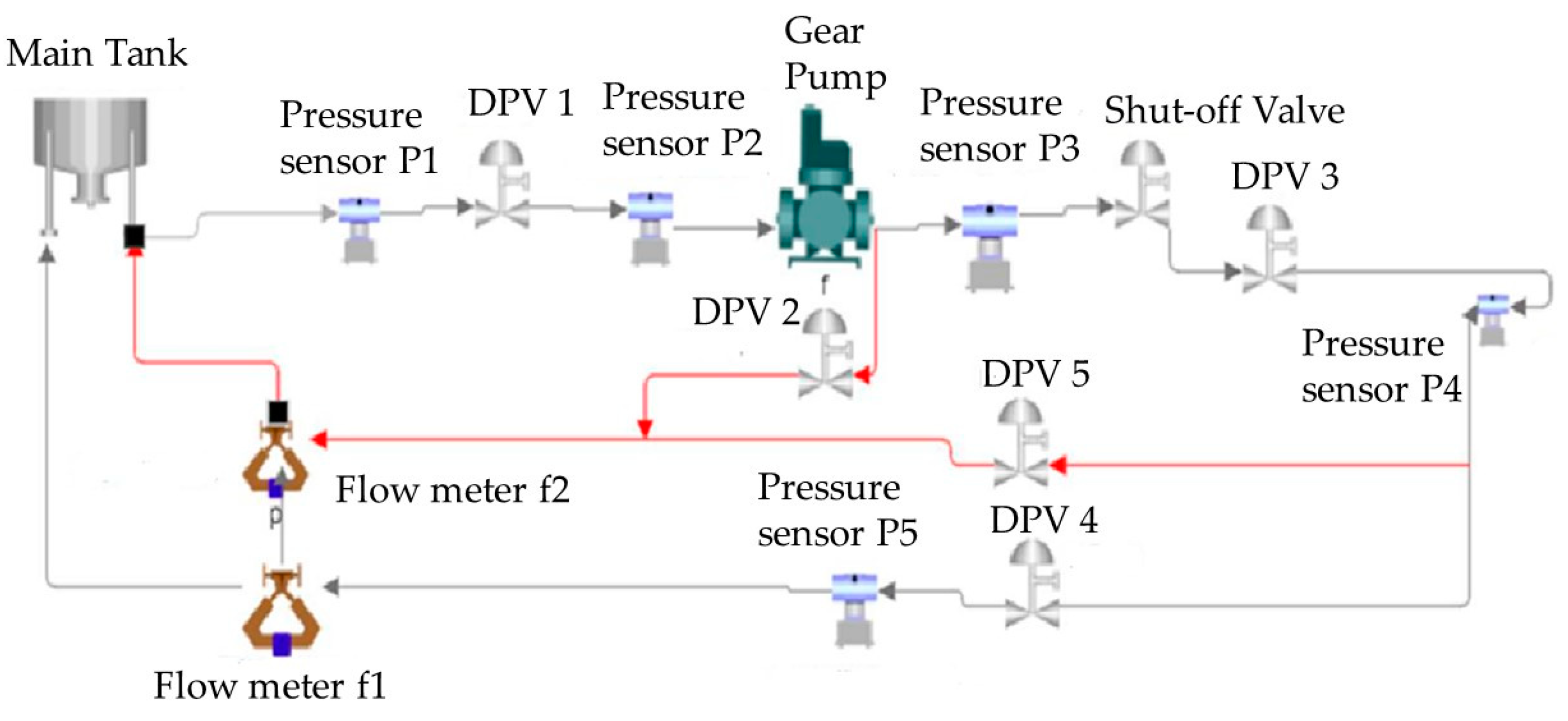
2.1.2. Description of the System under Investigation
2.1.3. Process Data Capture
2.1.4. Synthetic Data Generation
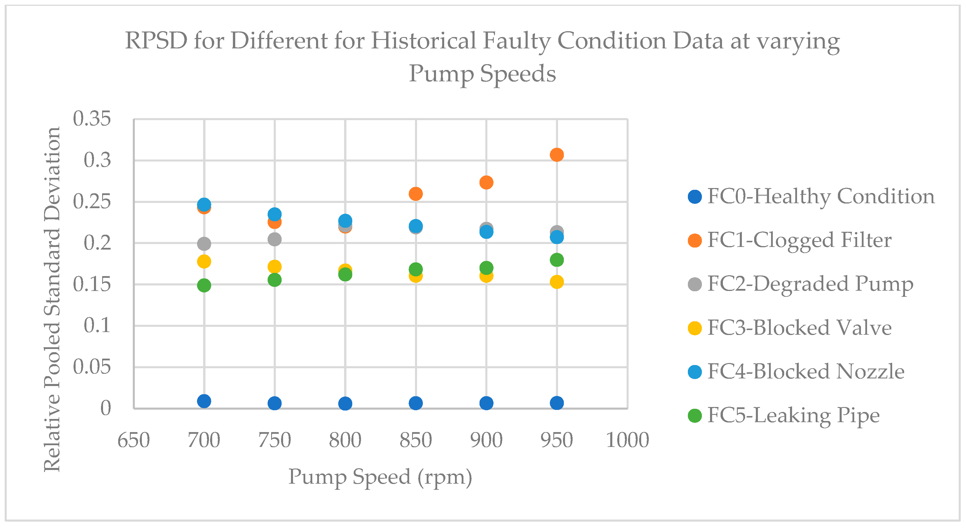
2.1.5. Relative Pooled Variance
2.1.6. Gage R&R Analysis
2.1.7. Earth Mover’s Distance
2.2. Component Degradation Characterisation
2.3. Fault Detection and Isolation (FDI)
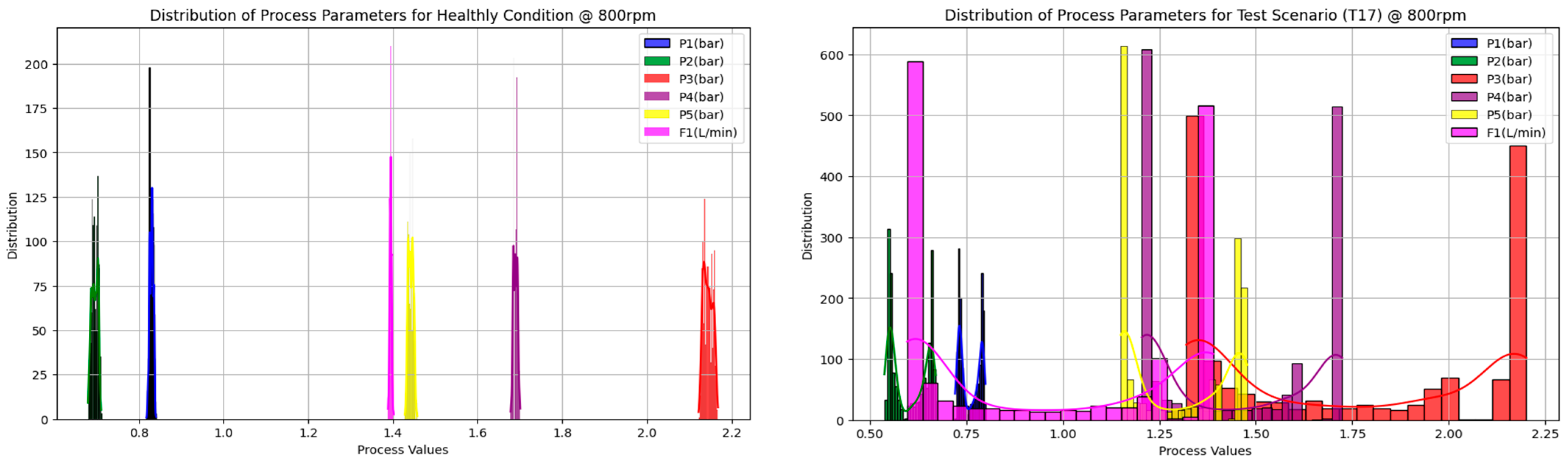
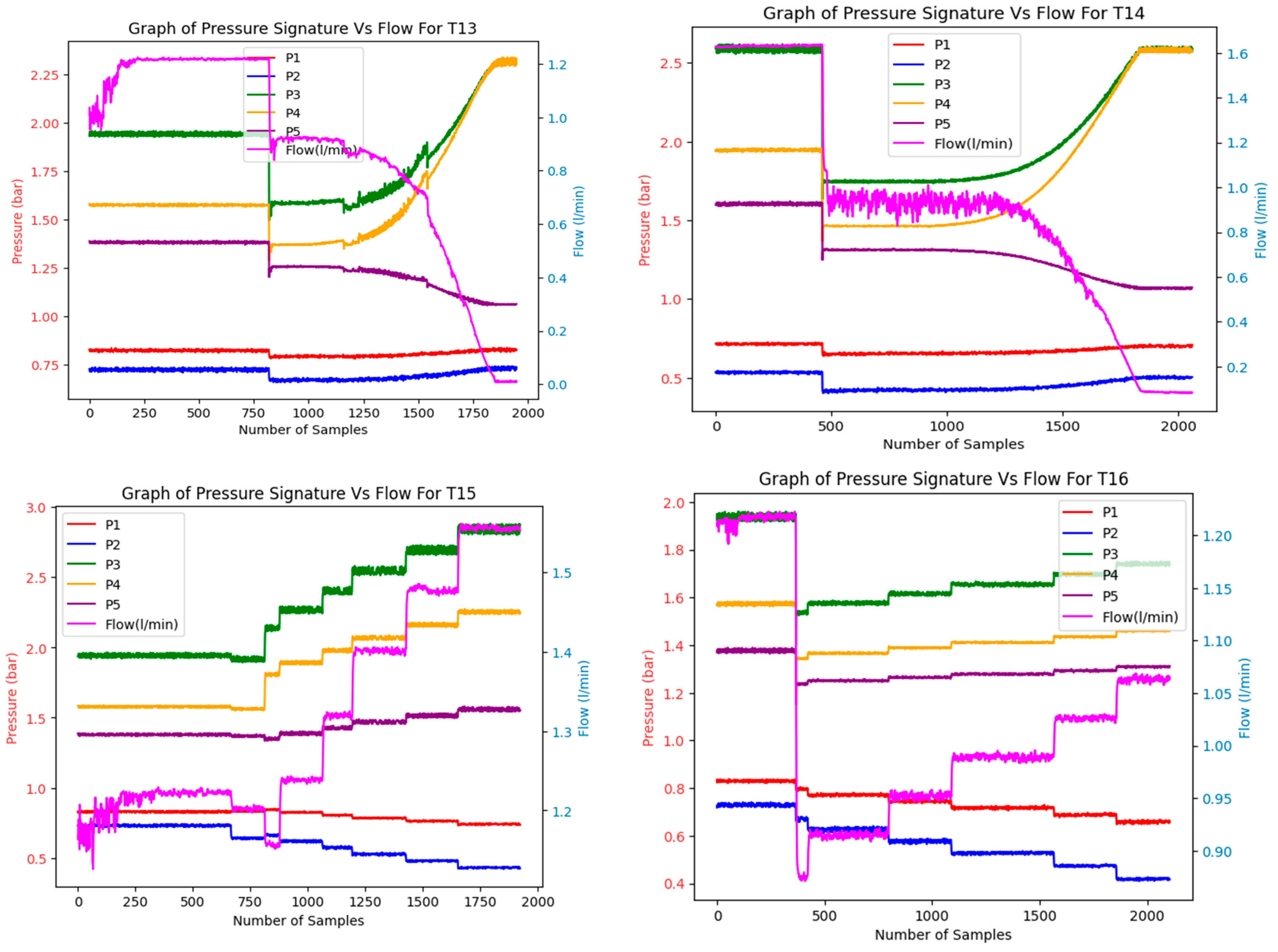
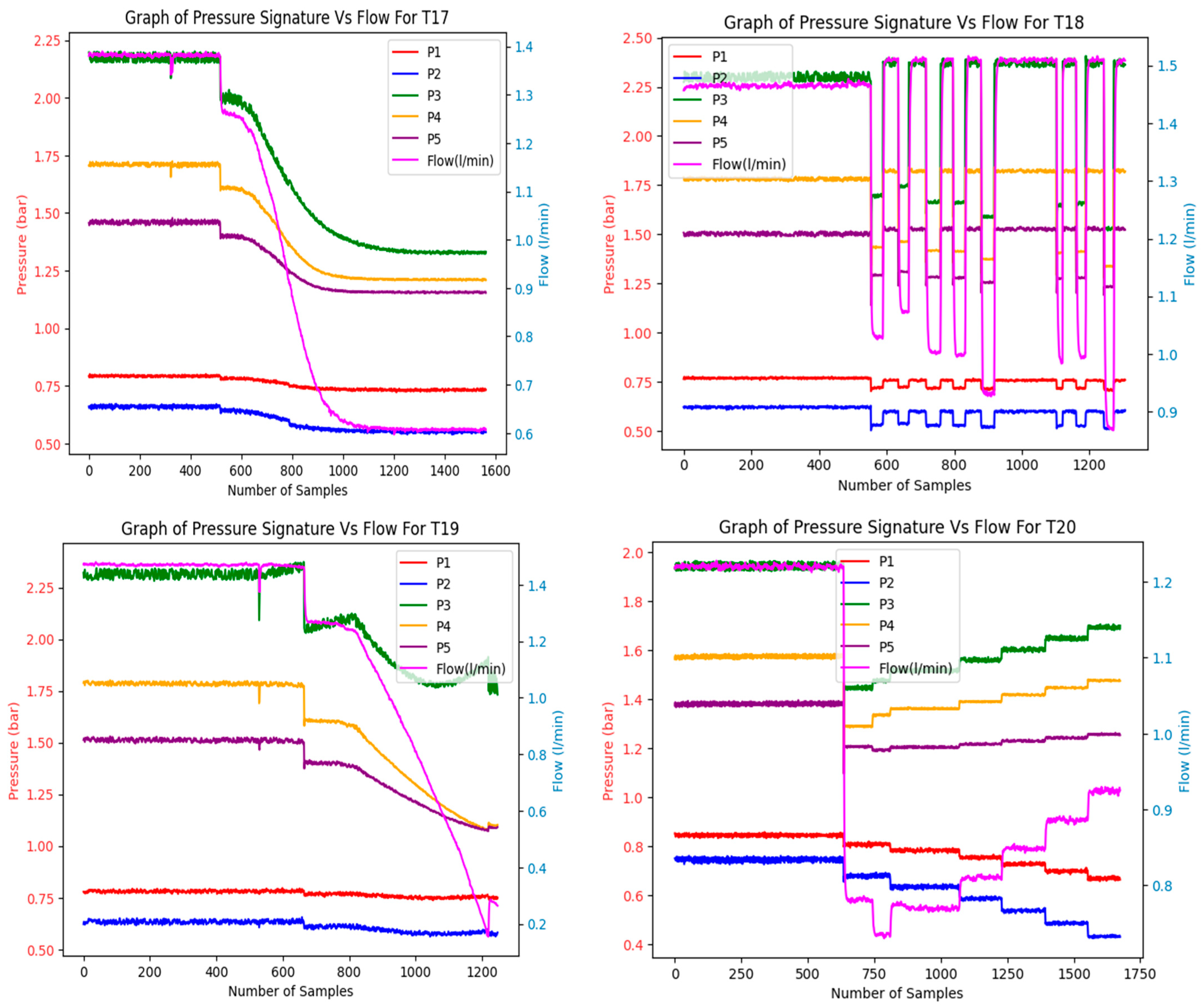
2.3.1. Test Degradation Scenarios
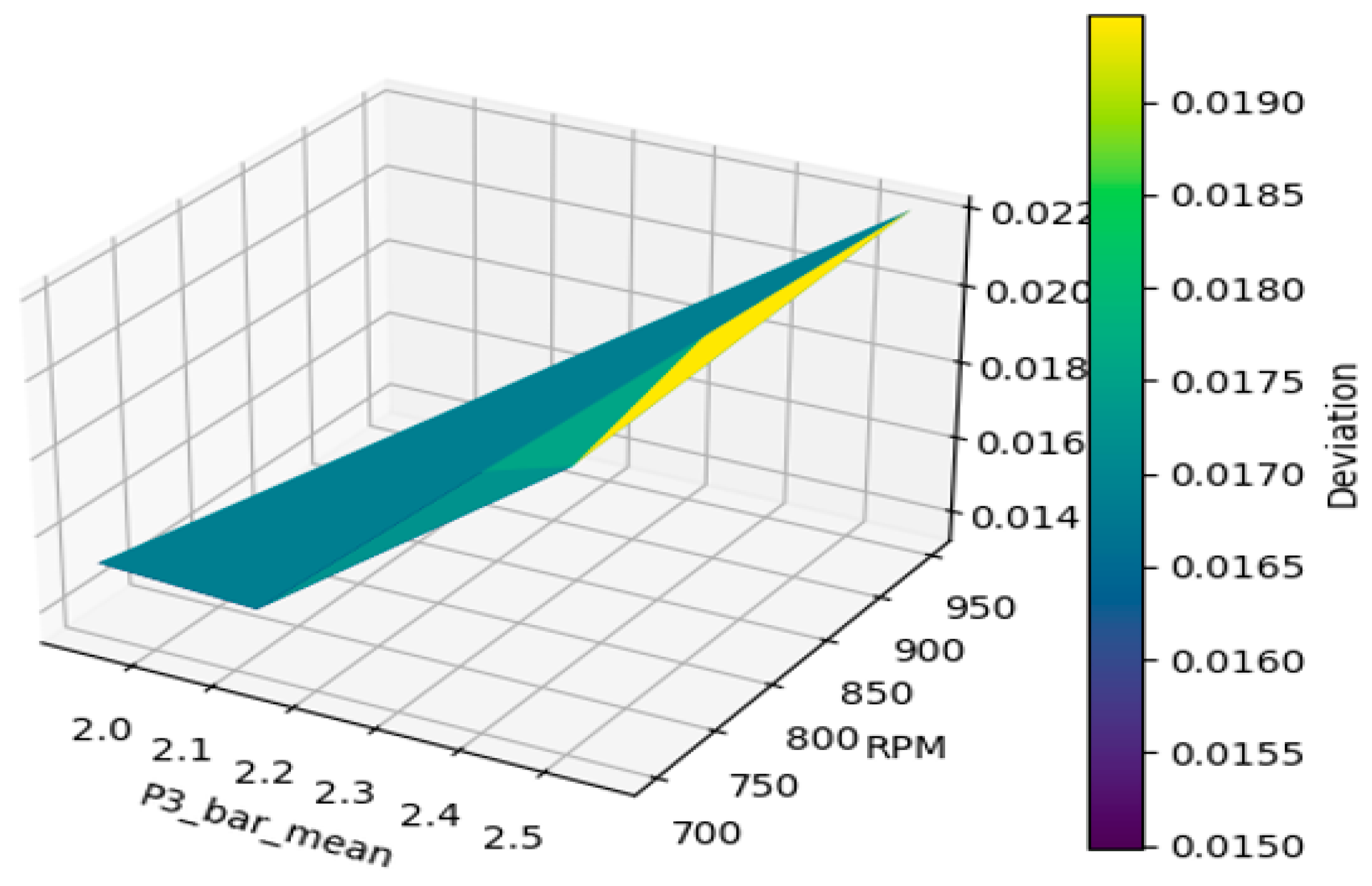
2.3.2. Statistical Process Control (SPC) Approach
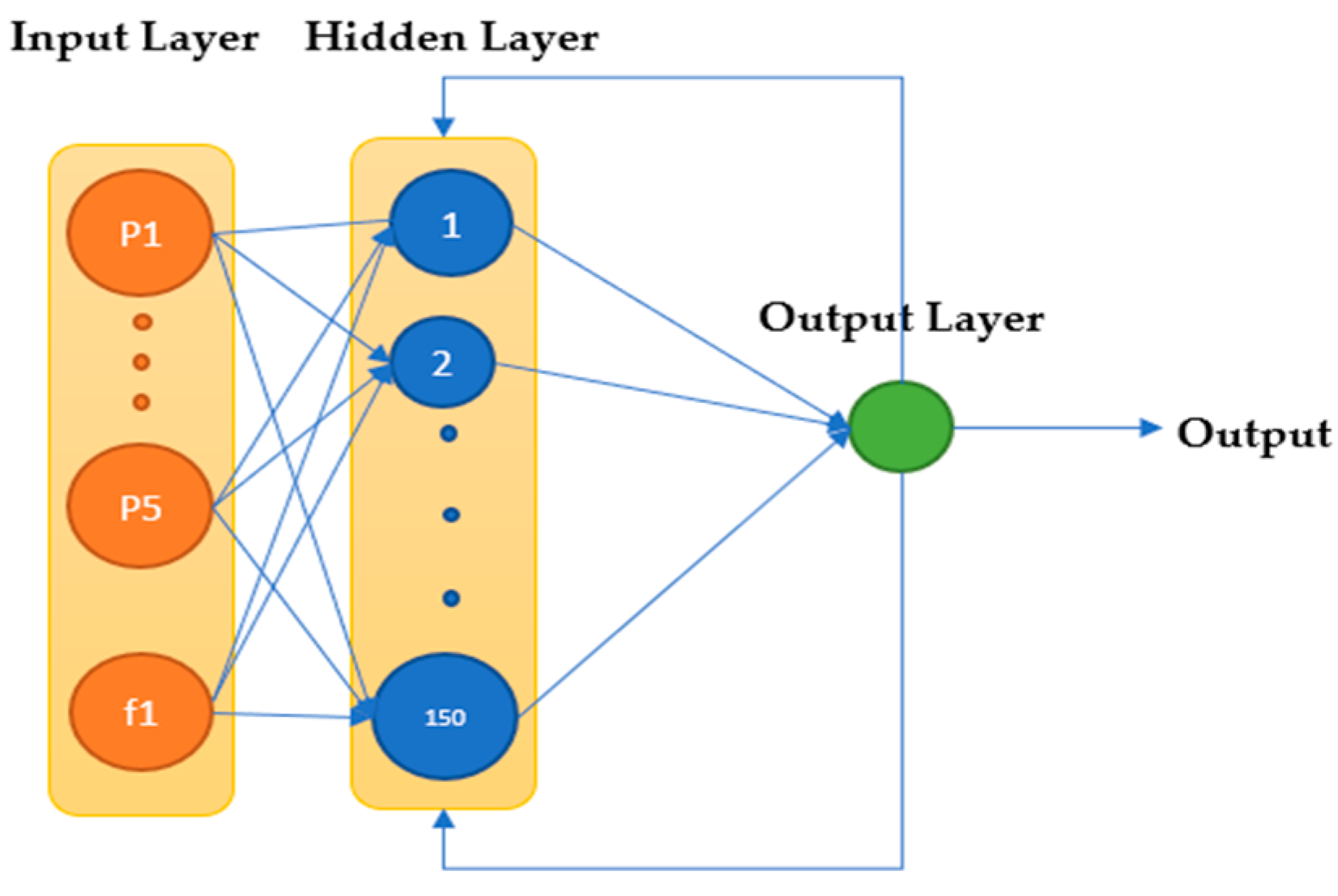
2.3.3. Data-Driven Approach
2.4. FDI Benchmarking Process
3. Results and Potential IIoT instantiation
3.1. Results and Findings
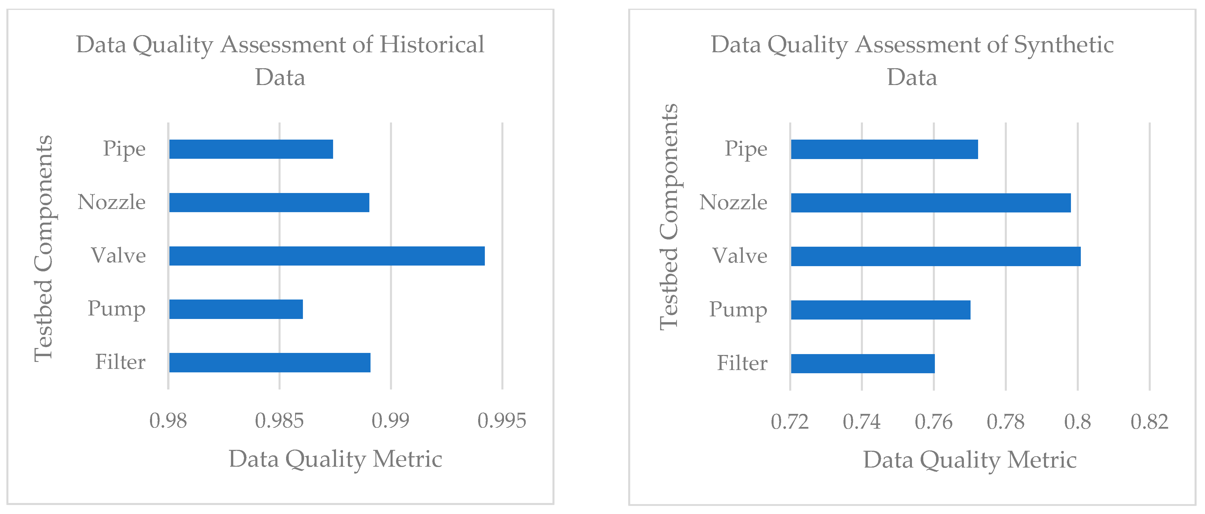
3.1.1. Measurement System Analysis
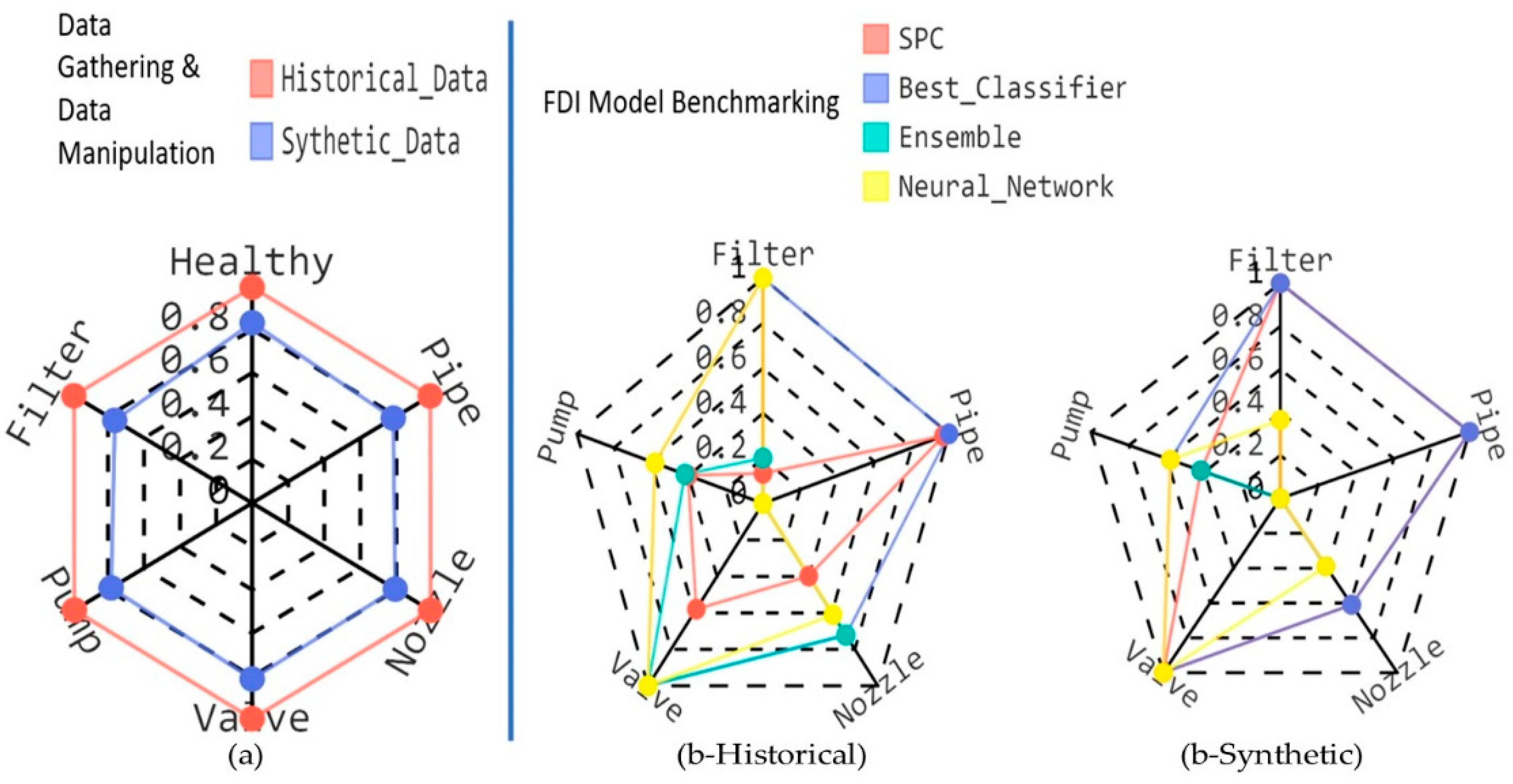
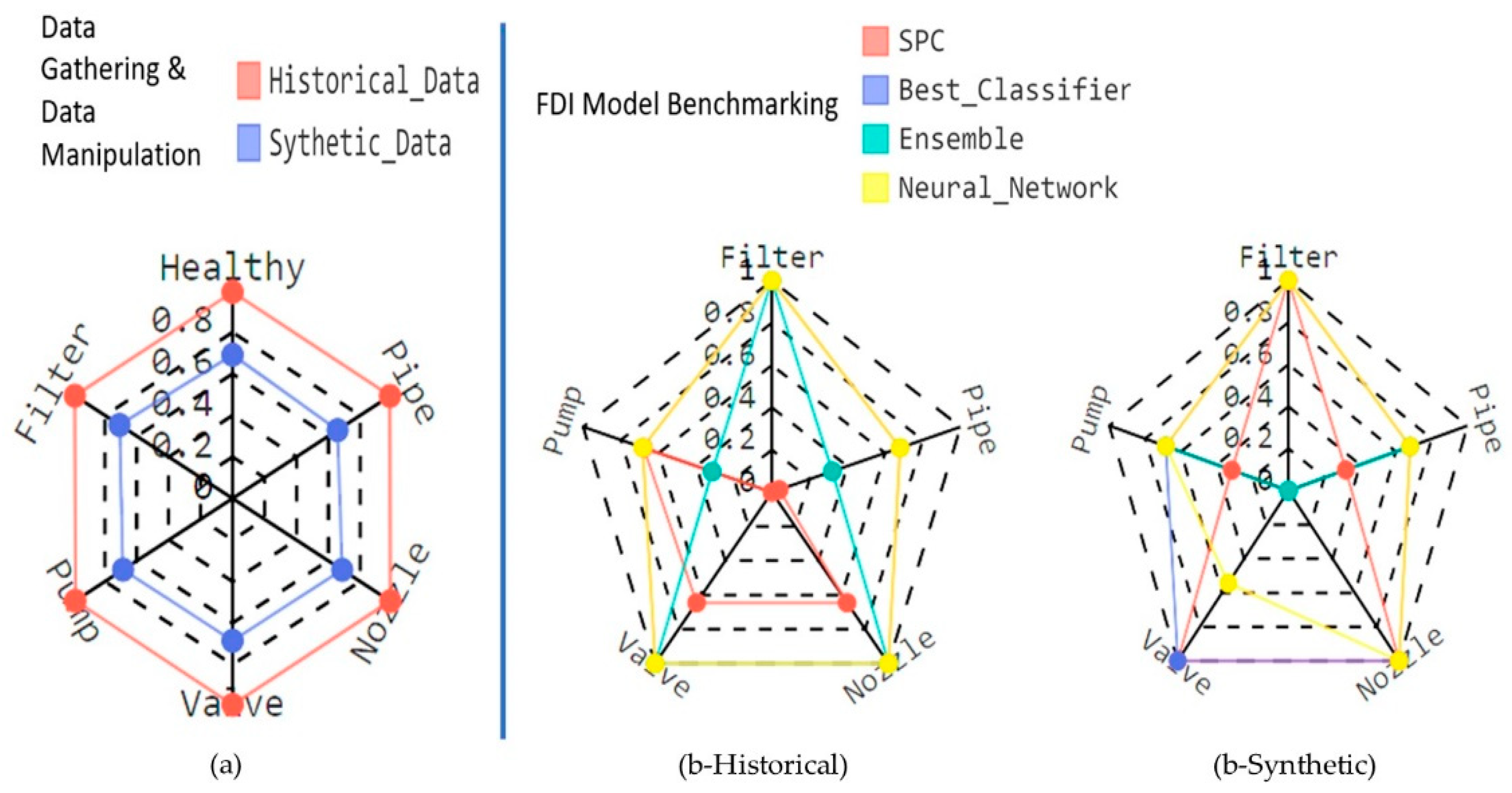
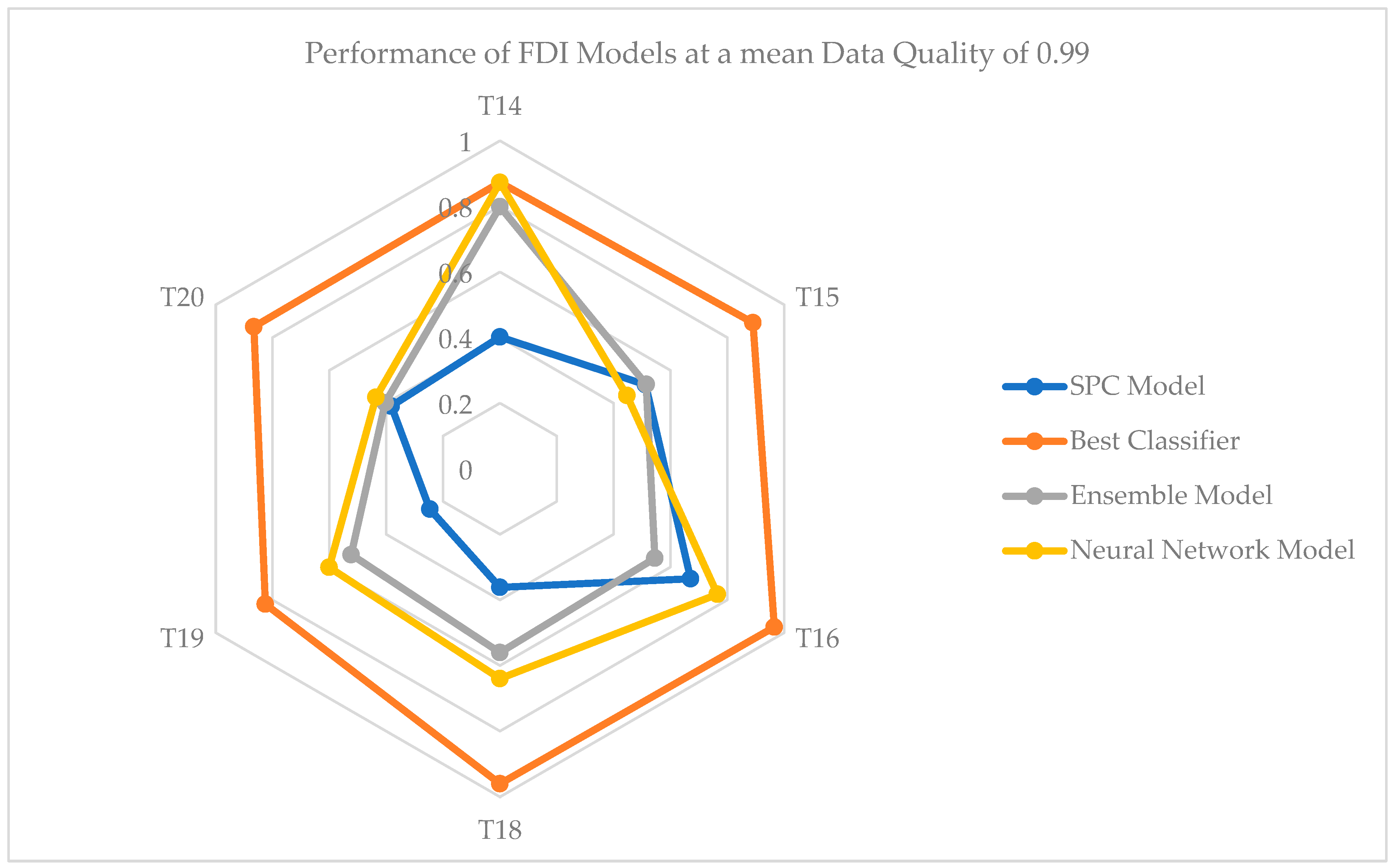
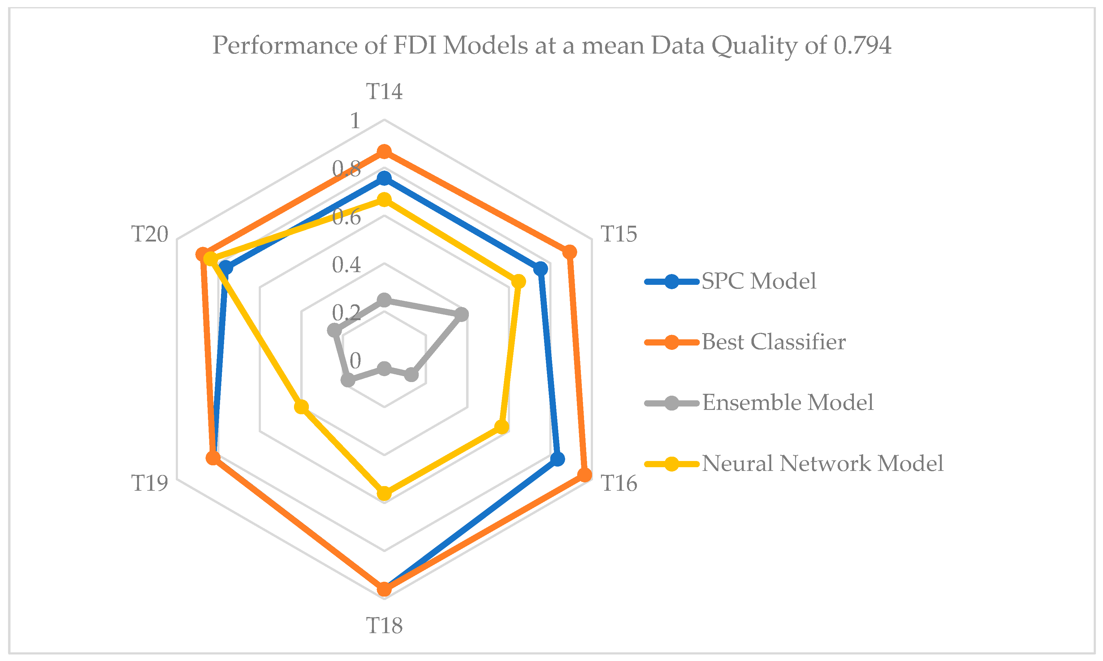
3.1.2. The Nexus between Data Quality and FDI Model Performance
3.1.3. Discussion
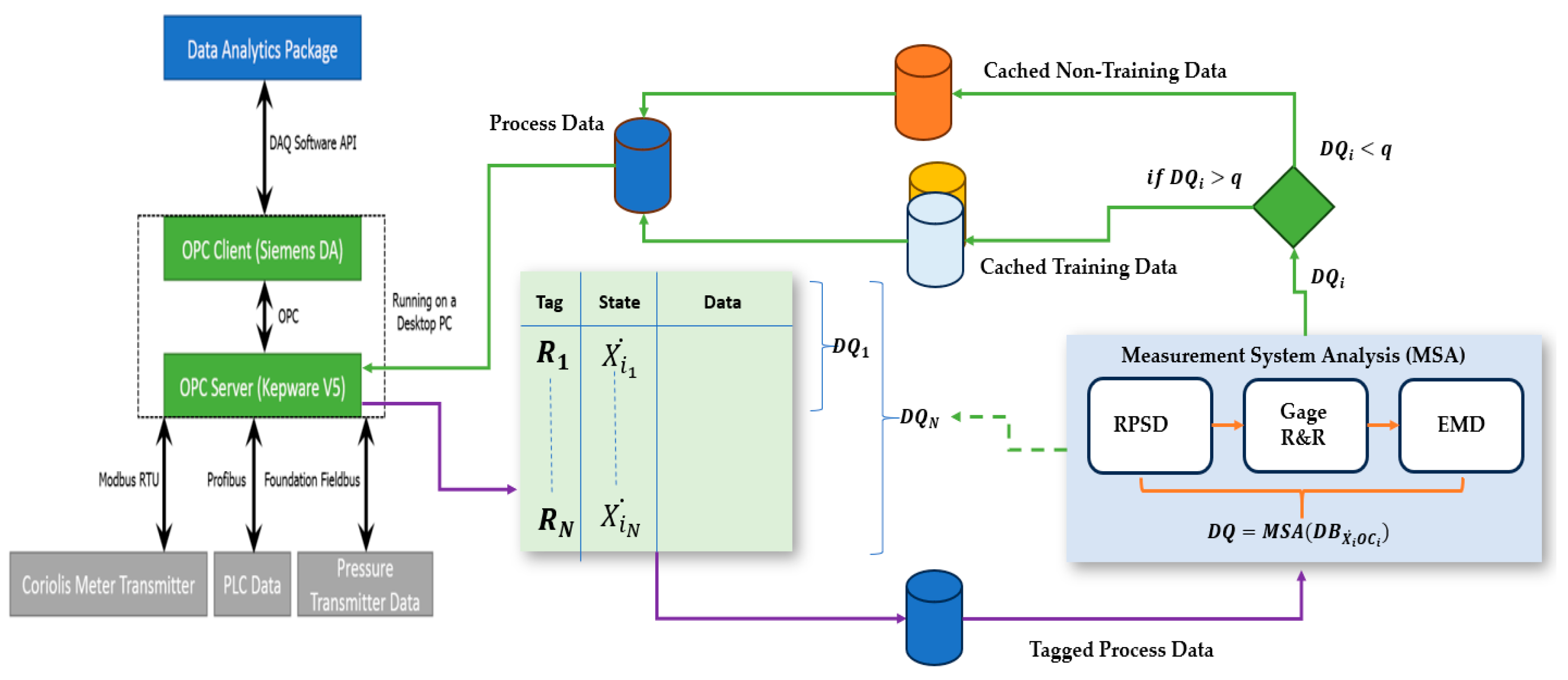
3.2. Potential IIoT Instantiation of the MSA Process
4. Concluding Remarks
Author Contributions
Funding
Institutional Review Board Statement
Informed Consent Statement
Data Availability Statement
Conflicts of Interest
Appendix A
Appendix A.1. Test Degradation Scenarios


Appendix A.2. Best Classification Algorithm for Each Component Ungergoing Component Degradation

| Test | Filter | Pump | Valve | Nozzle | Pipe |
|---|---|---|---|---|---|
| T13 | Logistic regression | Logistic regression | Logistic regression | Logistic regression | Decision tree classifier |
| T14 | Decision tree classifier | SVC | Logistic regression | Decision tree classifier | Logistic regression |
| T15 | Decision tree classifier | SVC | Logistic regression | Decision tree classifier | Gaussian NB |
| T16 | SVC | Decision tree classifier | Gaussian NB | SVC | SVC |
| T17 | Logistic regression | Decision tree classifier | Gaussian NB | Logistic regression | K neighbours classifier |
| T18 | SVC | Decision tree classifier | Decision tree classifier | Logistic regression | Decision tree classifier |
| T19 | Logistic regression | Decision tree classifier | Logistic regression | Decision tree classifier | SVC |
| T20 | SVC | Logistic regression | Logistic regression | Decision tree classifier | SVC |
| Test | Filter | Pump | Valve | Nozzle | Pipe |
|---|---|---|---|---|---|
| T13 | Logistic regression | Logistic regression | Decision tree classifier | Logistic regression | Logistic regression |
| T14 | Decision tree classifier | Decision tree classifier | Gaussian NB | Decision tree classifier | Gaussian NB |
| T15 | Decision tree classifier | Decision tree classifier | Decision tree classifier | Logistic regression | Decision tree classifier |
| T16 | SVC | Logistic regression | Decision tree classifier | Gaussian NB | Gaussian NB |
| T17 | Logistic regression | Logistic regression | Decision tree regressor | Decision tree regressor | Logistic regression |
| T18 | SVC | Logistic regression | Decision tree classifier | Decision tree classifier | Decision tree classifier |
| T19 | Logistic regression | Decision tree classifier | Decision tree classifier | Decision tree classifier | Decision tree classifier |
| T20 | SVC | Logistic regression | Logistic regression | Logistic regression | Logistic regression |
References
- Fuller, A.; Fan, Z.; Day, C. Digital Twin: Enabling Technologies, Challenges and Open Research. IEEE Access 2020, 8, 108952–108971. [Google Scholar] [CrossRef]
- Tao, F.; Qi, Q.; Wang, L.; Nee, A.Y.C. Digital twins and cyber–physical systems toward smart manufacturing and industry 4.0: Correlation and comparison. Engineering 2019, 5, 653–661. [Google Scholar] [CrossRef]
- Lu, Y.; Liu, C.; Kevin, I.; Huang, H.; Xu, X. Digital Twin-driven smart manufacturing: Connotation, reference model, applications and research issues. Robot. Comput. Integr. Manuf. 2020, 61, 101837. [Google Scholar] [CrossRef]
- Malakuti, S.; Grüner, S. Architectural aspects of digital twins in IIOT systems. In Proceedings of the 12th European Conference on Software Architecture: Companion Proceedings, Madrid, Spain, 24–28 September 2018; pp. 1–2. [Google Scholar] [CrossRef]
- Kuts, V.; Modoni, G.E.; Otto, T.; Sacco, M.; Tahemma, T.; Bondarenko, Y.; Wang, R. Synchronizing physical factory and its digital twin through an IIOT middleware: A case study. Proc. Est. Acad. Sci. 2019, 68, 364. [Google Scholar] [CrossRef]
- Souza, V.; Cruz, R.; Silva, W.; Lins, S.; Lucena, V. A digital twin architecture based on the industrial internet of things technologies. In Proceedings of the IEEE International Conference on Consumer Electronics (ICCE), Las Vegas, NV, USA, 11–13 January 2019; pp. 1–2. [Google Scholar]
- Delgado, J.M.D.; Odeyele, L. Digital Twins for the built environment: Learning from conceptual and process models in manufacturing. Adv. Eng. Inform. 2021, 49, 101332. [Google Scholar] [CrossRef]
- Yao, J.F.; Yang, Y.; Wang, X.C.; Zhang, X.P. Systematic review of digital twin technology and applications. Vis. Comput. Ind. Biomed. Art 2023, 6, 10. [Google Scholar] [CrossRef] [PubMed]
- Aghashahi, M.; Sela, L.; Banks, M.K. Benchmarking dataset for leak detection and localization in water distribution systems. Data Brief 2023, 48, 109148. [Google Scholar] [CrossRef] [PubMed]
- Fernandes, M.; Corchado, J.M.; Marreiros, G. Machine learning techniques applied to mechanical fault diagnosis and fault prognosis in the context of real industrial manufacturing use-cases: A systematic literature review. Appl. Intell. 2022, 52, 14246–14280. [Google Scholar] [CrossRef]
- Han, H.; Gu, B.; Hong, Y.; Kang, J. Automated FDD of multiple-simultaneous faults (MSF) and the application to building chillers. Energy Build. 2011, 43, 2524–2532. [Google Scholar] [CrossRef]
- Chandrashekar, G.; Sahin, F. A survey on feature selection methods. Comput. Electr. Eng. 2014, 40, 16–28. [Google Scholar] [CrossRef]
- Yang, J.; Guo, Y.; Zhao, W. Long short-term memory neural network based fault detection and isolation for electro-mechanical actuators. Neurocomputing 2019, 360, 85–96. [Google Scholar] [CrossRef]
- Khalid, S.; Khalil, T.; Nasreen, S. A survey of feature selection and feature extraction techniques in machine learning. In Proceedings of the 2014 Science and Information Conference, London, UK, 27–29 August 2014; IEEE: New York, NY, USA; pp. 372–378. [Google Scholar]
- Zhang, L.; Lin, J.; Liu, B.; Zhang, Z.; Yan, X.; Wei, M. A review on deep learning applications in prognostics and health management. IEEE Access 2019, 7, 162415–162438. [Google Scholar] [CrossRef]
- Burdick, R.K.; Borror, C.M.; Montgomery, D.C. A Review of Methods for Measurement Systems Capability Analysis. J. Qual. Technol. 2018, 35, 342–354. [Google Scholar] [CrossRef]
- Dina, A.S.; Siddique, A.B.; Manivannan, D. Effect of Balancing Data Using Synthetic Data on the Performance of Machine Learning Classifiers for Intrusion Detection in Computer Networks. IEEE Access 2022, 10, 96731–96747. [Google Scholar] [CrossRef]
- Hozo, S.P.; Djulbegovic, B.; Hozo, I. Estimating the mean and variance from the median, range, and the size of a sample. BMC Med. Res. Methodol. 2005, 5, 13. [Google Scholar] [CrossRef] [PubMed]
- Kazerouni, A.M. Design and analysis of gauge R&R studies: Making decisions based on ANOVA method. Int. J. Ind. Manuf. Eng. 2009, 3, 335–339. [Google Scholar]
- Rubner, Y.; Tomasi, C.; Guibas, L.J. The Earth Mover’s Distance as a Metric for Image Retrieval. Int. J. Comput. Vis. 2000, 40, 99–121. [Google Scholar] [CrossRef]
- Delouche, N.; Dersoir, B.; Schofield, A.B.; Tabuteau, H. Flow decline during pore clogging by colloidal particles. Phys. Rev. Fluid. 2022, 7, 034304. [Google Scholar] [CrossRef]
- Wahab, A. Analytical prediction technique for internal leakage in an external gear pump. Turbo Expo Power Land Sea Air 2009, 48869, 85–92. [Google Scholar]
- Ortega, R.; Metcalf, J.G.; Patton, C. Improving Operations of Inoperable Valves. In Infrastructure’s Hidden Assets, Proceedings of the Pipelines 2009, San Diego, CA, USA, 15–19 August 2009; American Society of Civil Engineers: Reston, VA, USA; pp. 1075–1082.
- Zhu, B.; Liu, Q.; Zhao, D.; Ren, S.; Xu, M.; Yang, B.; Hu, B. Effect of Nozzle Blockage on Circulation Flow Rate in Up-Snorkel during the RH Degasser Process. Steel Res. Int. 2016, 87, 136–145. [Google Scholar] [CrossRef]
- Abtew, M.A.; Kropi, S.; Hong, Y.; Pu, L. The Application of Using Statistical Process Control (SPC) Tools in Improving the Quality of a Manufacturing Process: A Case Study. Spektrum Ind. 2018, 11, 105–1142. [Google Scholar]
- Iqball, T.; Wani, M.A. Weighted ensemble model for image classification. Int. J. Inf. Technol. 2023, 15, 557–564. [Google Scholar] [CrossRef] [PubMed]
- Sperandei, S. Understanding logistic regression analysis. Biochem. Medica 2014, 24, 12–18. [Google Scholar] [CrossRef] [PubMed]
- Charbuty, B.; Abdulazeez, A. Classification based on decision tree algorithm for machine learning. J. Appl. Sci. Technol. Trends 2021, 2, 20–28. [Google Scholar] [CrossRef]
- Alam, M.S.; Vuong, S.T. Random Forest classification for detecting android malware. In Proceedings of the 2013 IEEE International Conference on Green Computing and Communications and IEEE Internet of Things and IEEE Cyber, Physical and Social Computing, Beijing, China, 20–23 August 2013; pp. 663–669. [Google Scholar] [CrossRef]
- Bafjaish, S.S. Comparative analysis of Naive Bayesian techniques in health-related for classification task. J. Soft Comput. Data Min. 2020, 1, 1–10. [Google Scholar]
- Kataria, A.; Singh, M.D. A review of data classification using k-nearest neighbor algorithm. Int. J. Emerg. Technol. Adv. Eng. 2013, 3, 354–360. [Google Scholar]
- Zhang, Y. Support vector machine classification algorithm and its application. In Proceedings of the Information Computing and Applications: Third International Conference, Chengde, China, 14–16 September 2012; Springer: Berlin/Heidelberg, Germany, 2012; pp. 179–186. [Google Scholar]
- Bentéjac, C.; Csörgő, A.; Martínez-Muñoz, G. A comparative analysis of gradient boosting algorithms. Artif. Intell. Rev. 2021, 54, 1937–1967. [Google Scholar] [CrossRef]
- Wang, R. AdaBoost for feature selection, classification and its relation with SVM, a review. Phys. Procedia 2012, 25, 800–807. [Google Scholar] [CrossRef]


| Component | Fault Emulation | Healthy State/Fault Emulation Mechanism | Fault Code |
|---|---|---|---|
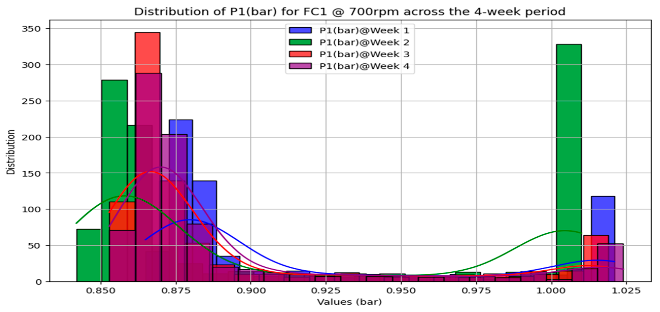
| Filter | DPV 1 | Fully open/gradually closing | FC1 |
| Pump | DPV 2 | Fully closed/gradually opening | FC2 |
| Valve | DPV 3 | Fully open/gradually closing | FC3 |
| Nozzle | DPV 4 | Fully open/gradually closing | FC4 |
| Pipe | DPV 5 | Fully closed/gradually opening | FC5 |
| Test Period | 4 Consecutive Weeks |
|---|---|
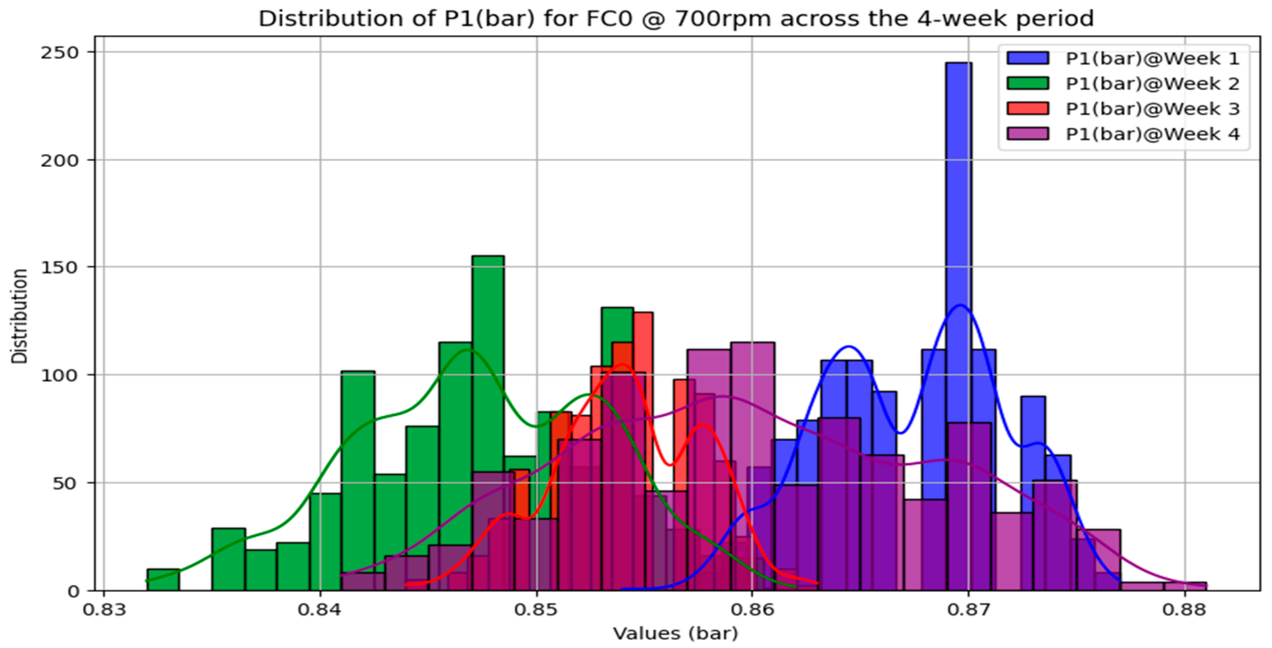
| Faulty condition scenarios (total No. of tests) | FC0—healthy condition (24) FC1—clogged filter (24) FC2—degraded pump (24) FC3—blocked valve (24) FC4—blocked nozzle (24) FC5—leaking pipe (24) |
| Pump speed (rpm) | 700/750/800/850/900/950 |
| Week | Nomenclature Test | FC0_700 | ………… | FC5_950 |
|---|---|---|---|---|
| 1 | Test campaign 1 | ………… | ||
| 2 | Test campaign 2 | ………… | ||
| 3 | Test campaign 3 | ………… | ||
| 4 | Test campaign 4 | ………… |
| MCD Test No. (Total No. of Tests) | Degradation Level (Component 1) (in Percentage of DPV Opening) | Degradation Level (Component 2) (in Percentage of DPV Opening) | Operational Speed Range (rpm) | Fault Combination |
|---|---|---|---|---|
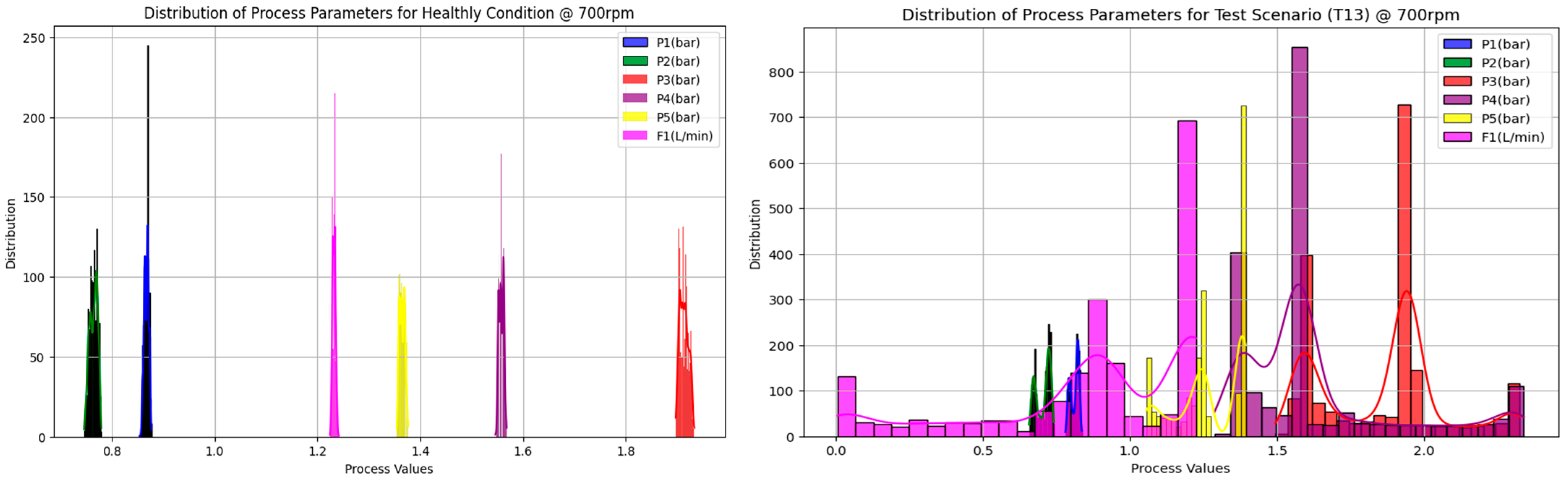
| T13 (1) | Pump (medium severity) at 45% | Constant degradation of nozzle (30–100% severity) | 700 | FC2 and FC4 |
| T14 (1) | Pump (medium severity) at 45% | Constant degradation of nozzle (30–100% severity) | 950 | FC2 and FC4 |
| T15 (1) | Filter (high severity) at 68% | Healthy condition (0% severity) | 700 to 950 | FC1 only |
| T16 (1) | Pump (medium severity) at 50% | Nozzle (medium severity) at 60% | 700 to 950 | FC2 and FC4 |
| T17 (1) | Constant degradation of pump (0–100% severity) | Constant degradation of pipe (0–100% severity) | 800 | FC2 and FC5 |
| T18 (1) | Intermittent faults for the pump between a 45% and 60% level of severity | Healthy condition (0% severity) | 850 | FC2 only |
| T19 (1) | Constant degradation of pump (0–100% severity) | Constant degradation of valve (30–100% severity) | 850 | FC2 and FC3 |
| T20 (1) | Pump (medium severity) at 55% | Nozzle (high severity) at 70% | 700 to 950 | FC2 and FC4 |
| Historical Dataset with Average Data Quality of 0.99 | ||||
|---|---|---|---|---|
| Model | SPC | Best Classifier | Ensemble | Neural Network |
| Mean accuracy (%) | 49.7 | 86.10 | 46.84 | 63.81 |
| Synthetic Dataset with Average Data Quality of 0.794 | ||||
| Model | SPC | Best Classifier | Ensemble | Neural Network |
| Mean accuracy (%) | 80.55 | 83.82 | 16.18 | 46.71 |
| Historical Dataset with Average Data Quality of 0.99 | ||||
|---|---|---|---|---|
| Model | SPC | Best Classifier | Ensemble | Neural Network |
| Mean accuracy (%) | 40.18 | 87.28 | 72.72 | 87.27 |
| Synthetic Dataset with Average Data Quality of 0.69 | ||||
| Model | SPC | Best Classifier | Ensemble | Neural Network |
| Mean accuracy (%) | 72.72 | 87.27 | 27.27 | 78.12 |
Disclaimer/Publisher’s Note: The statements, opinions and data contained in all publications are solely those of the individual author(s) and contributor(s) and not of MDPI and/or the editor(s). MDPI and/or the editor(s) disclaim responsibility for any injury to people or property resulting from any ideas, methods, instructions or products referred to in the content. |
© 2023 by the authors. Licensee MDPI, Basel, Switzerland. This article is an open access article distributed under the terms and conditions of the Creative Commons Attribution (CC BY) license (https://creativecommons.org/licenses/by/4.0/).
Share and Cite
Barimah, A.K.; Niculita, O.; McGlinchey, D.; Cowell, A. Data-Quality Assessment for Digital Twins Targeting Multi-Component Degradation in Industrial Internet of Things (IIoT)-Enabled Smart Infrastructure Systems. Appl. Sci. 2023, 13, 13076. https://doi.org/10.3390/app132413076
Barimah AK, Niculita O, McGlinchey D, Cowell A. Data-Quality Assessment for Digital Twins Targeting Multi-Component Degradation in Industrial Internet of Things (IIoT)-Enabled Smart Infrastructure Systems. Applied Sciences. 2023; 13(24):13076. https://doi.org/10.3390/app132413076
Chicago/Turabian StyleBarimah, Atuahene Kwasi, Octavian Niculita, Don McGlinchey, and Andrew Cowell. 2023. "Data-Quality Assessment for Digital Twins Targeting Multi-Component Degradation in Industrial Internet of Things (IIoT)-Enabled Smart Infrastructure Systems" Applied Sciences 13, no. 24: 13076. https://doi.org/10.3390/app132413076