Anomaly Detection for IOT Systems Using Active Learning

Abstract

The prevalence of Internet of Things (IoT) technologies is on the rise, making the identification of anomalies in IoT systems crucial for ensuring their security and reliability. However, many existing approaches rely on static classifiers and immutable datasets, limiting their effectiveness. In this paper, we have utilized the UNSW-NB15 dataset, which contains 45 variables including multi- and binary-target variables, to determine the most relevant properties for detecting abnormalities in IoT systems. To address this issue, our research has investigated the use of active learning-based algorithms for anomaly detection in IoT systems. Active learning is a powerful technique that improves precision and productivity by eliminating the need for labeling and adapting to dynamic IoT environments. Additionally, our study has combined feature engineering methods, active learning approaches, and a random forest classifier to construct a resilient anomaly detection model for IoT devices. The proposed model has outperformed several state-of-the-art techniques, achieving an impressive accuracy rate of 99.7%. By implementing a rigorous sampling procedure and leveraging the collaborative nature of the random forest technique, our model has demonstrated a notable level of precision with a weighted average accuracy of 0.995. The findings of the study offered empirical evidence, supporting the efficacy of our active learning methodology in identifying abnormalities in IoT systems. Moreover, our study provides valuable insights and recommendations for future research and development activities in this field. Overall, this research contributes to the advancement of anomaly detection techniques in IoT systems, further enhancing their security and reliability.

1. Introduction

Since the Internet of Things (IoT) is growing rapidly and connecting more devices, security is becoming a major concern. By 2023, IoT devices will exceed 30 billion [1,2]. Thus, efficient anomaly detection solutions are essential for IoT network integrity and reliability [3]. Anomaly detection is critical to IoT security systems’ identification and mitigation of network threats and abnormalities [4,5]. Conventional anomaly detection uses established rules or criteria [6]. However, the above methods often fail to account for IoT networks’ complexity and ever-changing properties, incorrectly identifying positive or negative results. In recent years, much emphasis has been given to active learning strategies to tackle these issues. For example, an algorithm selects samples to maximize information for expert labeling in active learning [7,8]. The algorithm can learn from smaller, tagged models using an iterative strategy, reducing the requirement for significant labeling and improving the anomaly detection system. The main goal of this work is to examine active learning methods for IoT anomaly detection.

IoT networks’ flexibility and active learning algorithms can improve anomaly detection and reduce false positives and negatives [9]. A publicly accessible benchmark dataset is used by the authors in [10] to assess ‘ensemble anomaly’ detection techniques. Records of both regular and malicious network traffic from different network segments are included in the collection. The testing of intrusion detection systems is considered appropriate due to its realistic portrayal of network activities [11]. The intrusion detection system (IDS) model was developed by researchers using bagging, boosting, and random forest (RF) [12]. These techniques combine algorithms with decision-making mechanisms to increase the accuracy and robustness of the system.

To reduce the dimensionality of the dataset and to improve detection efficacy, they employed feature selection [13]. Although the utility of ensemble approaches in IDS has been studied previously, it is still unknown whether or not these techniques can enhance IDS security. Ensemble models were shown to have improved accuracy, precision, recall, and F1-score in detecting unknown attacks [14]. According to the researchers, the feature selection enhanced the performance of the ensembled model. The selection qualities are necessary for intrusion detection to function. The results demonstrated that the significance of feature selection in IDS is that it outperforms single-algorithm models [15].

Additionally, a fog-based anomaly detection system created especially for IoT networks was introduced by the authors in [16]. By developing an anomaly detection system, the researchers were able to locate fog nodes [17]. This solution has the potential to decentralize an Internet of Things network with cloud architecture. The UNSW-NB15 dataset served as the foundation for the transformer model that was built for this investigation. The architecture of the model was created to identify unusual network activity in Internet of Things networks [18]. The model was trained using a variety of approaches, including supervised and unsupervised ones. Additionally, several metrics, including accuracy, precision, and recall, were used to evaluate the model’s performance. Their research revealed that this approach was remarkably accurate in identifying anomalies.

Furthermore, intrusion detection technologies can be hybrid, misuse-based, or anomaly-based [19,20]. The misuse-based approach builds signatures utilizing expert skills and domain knowledge. Then, it looks for a network data pattern matching one or more database signatures. The misuse-based approach has a low false-positive rate since it can identify intrusions that fit a database signature [21]. Suppose it cannot recognize unknown incursions that may not include any database patterns, especially if the attacker knows the database contains signatures. In that case, it may have a high false-negative rate. The misuse-based IDS must update database signatures and rules often to fix it.

However, the anomaly-based strategy first learns normal network behaviors and then finds anomalies that deviate from them [21]. The anomaly-based technique can detect new assaults [22]. Likewise, the machine teaches most network behaviors, with no explicit rules. If IDS rules are supplied, attackers are less likely to learn them and make their attacks invisible [23]. As any previously unforeseen activity can be considered an anomaly, however, the anomaly-based strategy can create many false alarms.

In a scholarly publication, the author [24] reported a study that demonstrated the application of a supervised machine learning (ML) approach for an IDS in the IoT domain. These authors utilized the application and transport layer features of the UNSW-NB15 dataset. The technique being suggested involved the categorization of network traffic into two distinct groups: dangerous and benign. This categorization is achieved through the utilization of a decision tree (DT) classifier. To assess the efficacy of the proposed methodology, a 10-fold cross-validation approach was employed. The findings indicated that the suggested methodology achieved a 98.58% level of accuracy. The machine learning subfield, active learning, emphasizes learning from a few training examples [25]. Since IDS labels take time, it is ideal for IDS design, but may be difficult to label invasions that have never occurred before. Active learning combines machine learning and domain experts. It can reduce labeling efforts and quickly develop a machine learning model for intrusion detection. Accordingly, the active learning architecture can quickly update the machine learning model for new network assaults [26,27,28,29].

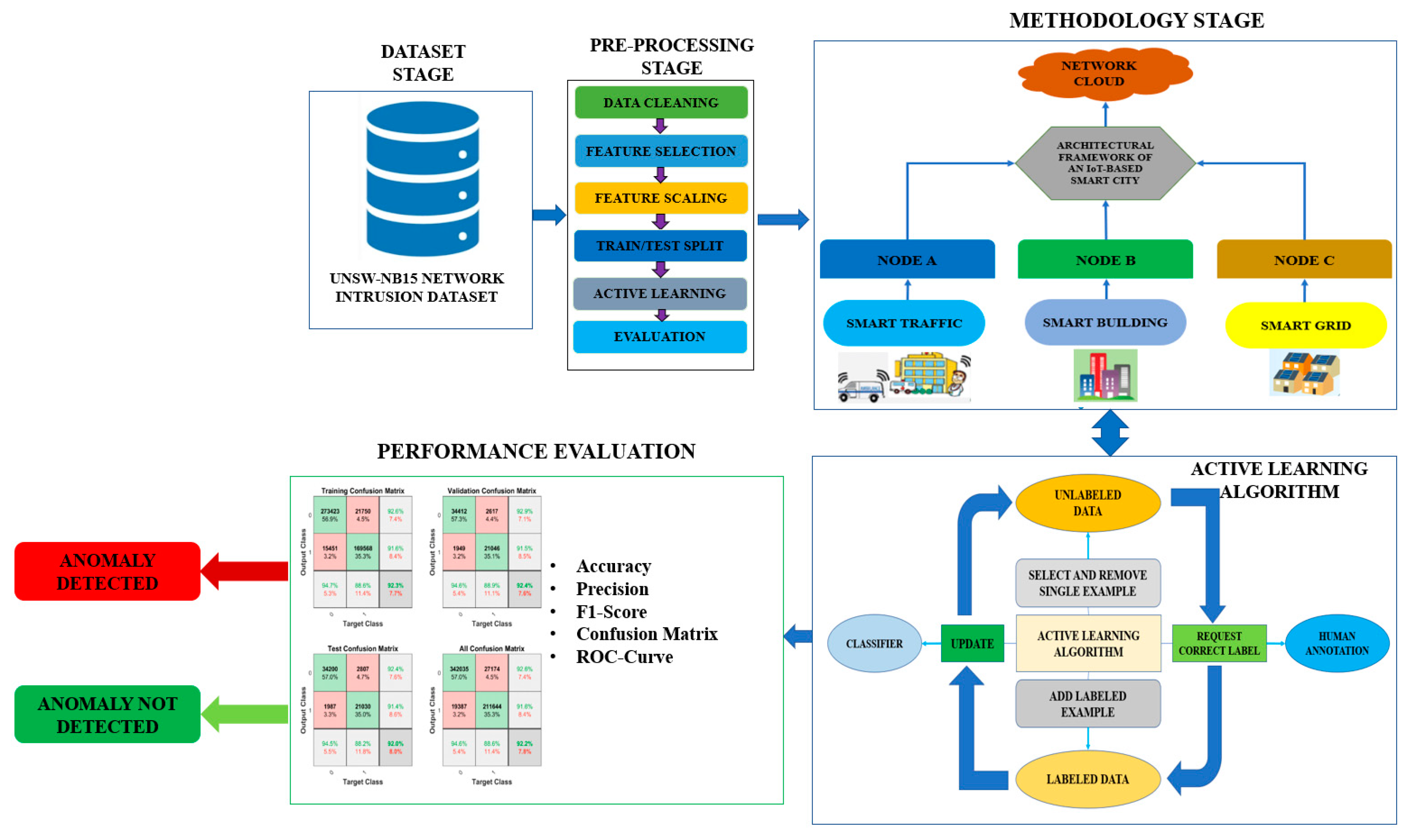
The diagram in Figure 1 illustrates a comprehensive framework utilized for anomaly detection in Internet of Things (IoT) systems, employing the active learning technique. The framework encompasses a series of fundamental stages, commencing with the first dataset phase, wherein the widely used UNSW-NB15 Network Intrusion Dataset is utilized. The initial data preparation phase includes crucial procedures such as data cleansing, selecting relevant features, normalizing features, and partitioning data into training and testing sets. The methodology section presents an architectural framework for a smart city based on the IoT, emphasizing the interconnection of nodes through smart traffic, buildings, and grids. The paper presents the technique for the active learning algorithm and the evaluation matrix used to assess its effectiveness. The evaluation matrix includes accuracy, precision, F1-score, a confusion matrix, and ROC curve. Ultimately, the final step of the process involves determining whether or not an anomaly has been found.

Moreover, the study presented in this paper makes several significant contributions:

• It proposes an active learning technique that is specifically tailored for anomaly detection. This technique considers the unique characteristics of anomaly detection and aims to improve the performance of anomaly detection models.
• Our model is evaluated on the UNSW-NB15 dataset, a publicly available dataset containing accurate network traffic data from an IoT device.
• It introduces a novel sampling strategy that is based on the concept of uncertainty. This strategy aims to select the most informative instances for labeling, thereby enhancing the learning process.
• We assess the efficacy of our active learning model by employing diverse feature selection methodologies, including mutual information-based feature selection, principal component analysis, and correlation-based feature selection.
• It develops a comprehensive framework, integrating active learning with random forest ensemble classifiers. This framework provides a systematic approach for incorporating active learning into the training of ensemble classifiers, which can lead to improved anomaly detection performance.
• The analysis of accuracy and other performance metrics is conducted on diverse benchmark IoT datasets to evaluate the effectiveness of the anomaly detection techniques.

The subsequent sections of the paper are organized in the following manner: Section 2 provides an overview of the background research conducted and highlights the pertinent studies conducted in this field. The process of data collecting is explicated in Section 3, the study technique is delineated in Section 4, and the findings and interpretations of the inquiry are examined in Section 5. Section 6 of the paper encompasses the discussion around our model, while Section 7 serves as a comprehensive summary and conclusion to the paper.

2. Literature Review

The proliferation of IoT devices has experienced a significant upswing in recent years [30], resulting in a substantial upsurge in the volume of data produced by these networked devices. The analysis of this extensive dataset is of the utmost importance for anomaly detection [31,32], as it facilitates the identification of atypical patterns or behaviors. Therefore, this literature review provides an overview of existing research that primarily focuses on active learning-based algorithms for anomaly detection in IoT systems. Various methodologies have also been investigated in this area.

According to [5], the utilization of an attack-specific characteristic, rather than an IoT-specific feature, might enhance the effectiveness and feasibility of a machine learning-based security system for attack detection and anomaly identification. The researchers employed the UNSW-NB15 and NSL-KDD datasets in this study. The performance of a system is evaluated by considering various metrics, including recall, precision, accuracy, F1-score, training time, and testing time. The F1-score of RFs is 0.99, whereas the Support Vector Machine (SVM) has an F1-score of 0.65. The primary aim of this study was to identify different types of attacks. The results obtained demonstrated a high level of accuracy in detecting various attacks, with a low occurrence of false alarms when utilizing the extracted features for this purpose.

According to [10], an inquiry was carried out to explore a method for anomaly identification in the context of improving cybersecurity in a smart city. To eliminate potential hazards and improve the overall security of the smart city infrastructure, the researchers used diverse methodologies such as K-Nearest Neighbor (KNN), Logistic Regression (LR), DT, artificial neural network (ANN), and RF. Their paper analyzes ensemble techniques, such as bagging and boosting, to improve the detection the architecture’s security. Their research is centered on using two datasets, namely UNSW-NB15 and CICIDS 2017. The results showed that the SVM achieved an accuracy rate of 90.50%. The artificial neural network had a classification accuracy of 79.5%, whereas the boosting approach had an accuracy rate of 98.6%, and the stacking method had an approximate accuracy rate of 98.8%. Therefore, the experimental results acquired using the dataset UNSW-NB15 can be used as a primary lead for identifying infrequent attacks in a smart city’s IoT environment.

The authors of [14] proposed a comprehensive framework for implementing the Variational Long Short-Term Memory (VLSTM) model, which involves the utilization of both estimation and compression networks. The researchers developed a VLSTM learning model for intelligent anomaly detection. This model utilizes rebuilt feature representations to address the challenge of balancing dimensionality reduction and feature retention in imbalanced Industrial Big Data (IBD) datasets. The experimental findings, encompassing the VLSTM strategy, outperformed six alternative approaches on the testing dataset, as evidenced by an F1-score of 0.907, a False Alarm Rate (FAR) value of 0.117, and an Area Under Curve (AUC) metric of 0.895. The findings demonstrate that, in comparison to baseline methods, their approach can successfully identify true abnormalities from data on typical network traffic and dramatically lower the false anomaly detection rate.

In addition, [16] described a new intrusion detection model that could be applied to fog nodes. This model used UNSW-NB15 properties to find superfluous IoT device traffic. This paper presents the tab transformer model, which surpasses machine learning. Said model distinguishes normal from irregular traffic at 98.35% accuracy. However, their approach predicts attacks with 97.22% accuracy across many classes. The model opened up new fog node anomaly study avenues, according to the review [19]. Furthermore, Kocher and Kumar [20] presented a variety of intrusion detection techniques. Their work trained ML classifiers using the UNSW-NB15 dataset. The study tested Naive Bayes (NB), LR, KNN, and RF to detect intrusion. Classifier accuracy, precision, recall, F1-score, Mean Squared Error (MSE), False Positive Rate (FPR), and True Positive Rate (TPR) were tested with and without feature selection procedures. These machine learning classifiers were also compared and according to the findings, the RF algorithm uses all of the information that is accessible to it to obtain an accuracy of 99.5%; when only certain features are used, the accuracy rises to 99.6%.

To build accurate IDSs, [22] developed the XGBoost method as a form of feature selection in conjunction with several ML approaches, including DT, LR, ANN, KNN, and SVM. To compare methods, the researchers used the UNSW-NB15 dataset. The experimental results demonstrate that by adopting the XGBoost-based feature selection strategy, methods like DT may increase their test accuracy in binary classification from 88.13% to 90.85%.

Similarly, [24] used features from the UNSW-NB15 dataset to discover sets of features based on flow, Message Queuing Telemetry Transport (MQTT), and Transmission Control Protocol (TCP). Overfitting, the curse of dimensionality, and dataset imbalances were all eliminated. To train the clusters, they used supervised machine learning techniques like ANN, SVM, and RF. The authors’ RF-based binary classification accuracy was 98.67%, while their multi-class classification accuracy was 97.37%. Using RF on Flow and MQTT features, TCP characteristics, and the best features from both clusters, they achieved classification accuracies of 96.74%, 91.96%, and 96.56%, respectively, using cluster-based approaches. They also show that the suggested feature clusters outperform other state-of-the-art supervised ML algorithms in terms of accuracy and training time.

The implementation of distributed deep learning approaches for the detection of IoT threats has highlighted recent developments in the field of IoT security (Parra et al., 2020) [25]. In addition, artificial intelligence has become a crucial tool for spotting irregularities in energy use in buildings, according to a thorough analysis of the latest developments and prospects by Himeur et al. [26]. A hierarchical hybrid intrusion detection system developed specifically for IoT applications was also suggested by Bovenzi et al., demonstrating the expanding variety of IoT security measures [27]. The use of semi-supervised hierarchical stacking temporal convolutional networks has also shown promise in anomaly detection for IoT connectivity, as Cheng et al. have shown [28]. Additionally, Pajouh et al. created a two-layer dimension reduction and two-tier classification model for anomaly-based intrusion detection in IoT backbone networks, highlighting the significance of strong security measures in the IoT ecosystem [29].

This literature review section has examined and evaluated different methodologies that have been proposed to tackle anomaly detection in IoT systems. Furthermore, traditional approaches are frequently needed to help in accommodating IoT environments’ ever-changing and dynamic nature, where anomalies may exhibit varying appearances over time. In summary, this literature analysis has underscored the importance of the various methodologies employed in identifying anomalies within IoT systems. Our proposed active learning methods can potentially improve the accuracy and efficiency of anomaly detection by eliminating the need for labeling and allowing for flexibility in dynamic IoT environments. The primary objective of this research article is to make a valuable contribution to the existing pool of knowledge in this particular field. Doing so will establish a solid groundwork for potential future developments in the domain of IoT anomaly detection, explicitly focusing on the utilization of active learning techniques.

Table 1. List of past references, including datasets/parameters, methodology, limitations, and results.

Ref.	Dataset/Parameters	Methodology	Limitations	Results
[5]	- Datasets like UNSW-NB15 and NSL-KDD were used. - In this way, 71,537,674 Denial of Service (DoS) incidents yield 25,000 random samples. From 75 Comma-Separated Values (CSV) files containing 1,821,639 information-gathering incidents, 25,000 are randomly extracted, and 1587 of those are theft occurrences. In total, 6430 are retrieved from 75 files containing 9543 normal instances.	- Machine learning algorithms include KNN, RF, SVM, and LR.	- A relatively small sample size was used for evaluating the proposed active learning approach for wireless IoT intrusion detection. - Does not provide information on the number of instances or the diversity of the dataset used. - Lacks of evidence of a real-world implementation of the proposed approach	- SVM: Precision of 92.6%. F1-score of 0.65. - KNN: Precision of 97.8%, F1-score of 0.99.
[10]	- The study evolves around two datasets, UNSW-NB15 and CICIDS2017. - The first dataset consists of approximately 2 million entries. - A total of 25,070 samples were used for testing and 13,961 samples for training. - The second dataset has 2,720,634 records in its sample space and 77 features.	- Machine learning techniques used in this model include RF, KNN, ANN, and SVM.	- Limited dataset for evaluating the effectiveness of ensemble techniques for anomaly detection. - Absence of a comparative analysis with other existing methods for intrusion detection.	- Accuracy for SVM is around 90.5%. - Accuracy for DT is 70.4%, RF is 91%, and 79.5% for ANN.
[14]	- To investigate the proposed VLSTM model, the UNSW-NB15 dataset is used. - Approximately 42 features are included in the dataset.	- Machine learning models like LSTM, NB, RF, AdaBoost, and Convolutional Neural Network (CNN) are used.	- Lacks practical implementation and validation in real-world industrial scenarios. - Does not provide a comprehensive comparison with existing anomaly detection algorithms or alternative techniques.	- For VLSTM, the validation dataset precision is 96.7%, and for the testing dataset the precision is 86%.
[16]	- The authors have employed the UNSW-NB15 dataset. - There are 45 network attributes in the dataset overall, including properties based on networks and flow. Other classifications include flow, fundamentals, substance, time, and other generated features. - With 175,341 training and 82,331 testing records in CSV format, the dataset has almost 2.5 million records in total.	- Binary classification via Machine Learning models like RF, LR, KNN, DT, and 1D-CNN.	- The research paper lacks details on testing scenarios, comparisons with existing anomaly detection techniques in fog computing architectures, and comprehensive evaluation metrics for the custom tab transformer’s performance, hindering understanding of its strengths and weaknesses. - The evaluation metrics utilized in the research paper to assess the performance of the custom tab transformer for anomaly detection in fog computing architectures are not fully comprehensive.	- RF accuracy of 96%, DT accuracy of 96.5%. A 1D-CNN accuracy of 96.8%.
[20]	- The UNSW-NB15 dataset is used. - This dataset contains approximately 49 attributes.	- Classifiers like NB, RF, LR, and KNN are used. - Performance metrics include precision, Mean-square error, F1-score, and accuracy.	- The research paper does not compare the performance of the machine learning algorithms with feature selection using the UNSW-NB15 dataset against other well-known intrusion detection datasets. - The paper focuses on the evaluation of the machine learning algorithms’ performance with feature selection but does not provide an in-depth analysis of the interpretability of the selected features.	- Accuracy of KNN: 98.28%. - Accuracy of NB: 76.59%. - Accuracy of LR: 98.4%. - Accuracy of RF: 99.5%.
[22]	- The UNSW-NB15 dataset is used. - It contains 42 features with 39 numeric and 3 non-numeric instances.	- Machine learning techniques like LR, ANN, DT, SVM, KNN, and XGBoost are used.	- The research paper does not provide a comprehensive comparison of the performance analysis of the IDS using different feature selection methods or other datasets. - The lack of practical implications restricts the usefulness of the research paper for practitioners looking for actionable insights to improve the efficiency and effectiveness of their IDS systems in real-world scenarios.	- With 42 features, SVM precision is 94.3%. DT has a precision of 96.5%. - LR has a precision of 98.9%.
[24]	- The UNSW-NB15 dataset is used. - It contains approximately 27 features instead of 47, with 24,596 packets for the training set and 68,264 packets of internet traffic.	- Machine learning uses techniques like RF, NB, ANN, DT, KNN, SVM, and ANN.	- Their dataset may have limitations in terms of representing a diverse and comprehensive collection of real-world IoT network traffic data. - Chosen ML algorithms might not be suitable for detecting emerging or previously unseen intrusion patterns. - Reliance on these specific layers may overlook potential attacks at other layers, leading to potential vulnerabilities in the IoT system.	- RF has an accuracy of 98.7%. - SVM has an accuracy of 97.7%. - ANN has an accuracy of 94.7%.

presents a comprehensive compilation of previous references, encompassing datasets, parameters, techniques, and corresponding outcomes.

3. Data Collection

The UNSW-NB15 dataset, used in the research papers [7,8] was curated by the Network Security Research Lab (NSRL) of the University of New South Wales (UNSW) in Sydney, Australia [33,34]. The dataset was created by simulating a real-world network environment, complete with numerous IoT devices, threats, and network traffic. The dataset comprises 2.5 million network flows containing both legitimate and criminal activities. The data was collected by monitoring a testbed network comprising three physical computers hosting diverse network services alongside twelve virtual machines running different operating systems. Virtual machines utilized various services and protocols, including the Hypertext Transfer Protocol (HTTP), Simple Mail Transfer Protocol (SMTP), Domain Name System (DNS), File Transfer Protocol (FTP), Secure Shell (SSH), Telecommunication Network (Telnet), Internet Control Message Protocol (ICMP), and TCP.

The Wireshark packet capture tool was employed to record the network traffic [35]. Subsequently, the data was pre-processed to eliminate relevant information for anomaly identification.

• UNSW-NB15_1.csv, UNSW-NB15_2.csv, UNSW-NB15_3.csv, and UNSW-NB15_4.csv are the four CSV files that make up the dataset. These files include 2,540,044 records overall.
• UNSW-NB15_LIST_EVENTS.csv is the file name for the list of events, and UNSW-NB15_GT.csv is the table name for the ground truth data.
• The UNSW_NB15_training-set.csv and UNSW_NB15_testing-set.csv portions of the dataset were utilized as the training and testing sets, respectively. A total of 175,341 records make up the training set, while 82,332 records from the attack and normal categories make up the testing set.

3.1. Data Description

Network intrusion detection often uses the UNSW-NB15 dataset as a labeled dataset [36]. It is frequently used to assess how well intrusion detection systems are performing. On the other hand, the data on network traffic is produced in the simulated network environment that makes up the dataset. This dataset contains both common operational tasks and a range of network assaults. The dataset is made up of both raw and processed data that has been given various network traffic indicators. As shown in

Table 2. UNSW testing data frame.

ct_flw_http_mthd	ct_src_1tm	ct_srv_dst	is_sm_ips_ports	attack_cat	Label
0	1	2	0	Normal	0
0	1	2	0	Normal	0
0	1	3	0	Normal	0
0	2	3	0	Normal	0
0	2	3	0	Normal	0

, these metrics consist of protocol, source, and destination IP addresses, port numbers, and packet and byte counts.

A total of 2,540,044 occurrences have been recorded and categorized into ten distinct classifications of network traffic, encompassing both routine traffic and nine distinct forms of attacks. The subsequent classifications represent a selection of attacks:

• Fuzzers;
• Exploits;
• Generic;
• Reconnaissance;
• Shellcode;
• Worms;
• Analysis;
• Backdoors;
• DoS.

The dataset comprises 45 variables, with the last two categorized as multi- and binary target variables. The initial 43 elements encompass a diverse range of characteristics, with the potential for certain ones to be omitted while others have significant importance.

The subsequent section provides a comprehensive account of each variable in the training dataset. The variables of the UNSW-NB15 dataset are delineated in the following list:

• id: a unique label for each flow.
• Dur: the flow’s time frame, measured in seconds.
• Proto: the flow’s protocol (such as Transmission Control Protocol (TCP), User Datagram Protocol (UDP), or ICMP).
• Service: the flow’s associated service (if any), such as HTTP, SSH, or FTP.
• State: the flow’s current condition, such as FIN-WAIT-1 or ESTABLISHED.
• spkts: the total number of packets the source host transmitted throughout the flow.
• dpkts: the total number of packets the destination host transmitted throughout the flow.
• sbytes: the total amount of data the source host transmits throughout the flow.
• dbytes: the total amount of data the destination host transmits throughout the flow.
• Rate: the flow’s average packet sending speed, expressed in packets per second.
• sttl: the value of the flow’s initial packet’s source Time to Live (TTL).
• dttl: the first packet in the flow’s destination TTL value.
• Sload: the rate in bytes per second at which the source host sends data during a flow.
• Dload: the rate in bytes per second at which the destination host sends data during the flow.
• Sloss: the total number of packets the source host lost along the flow.
• Dloss: the number of packets the destination host dropped along the flow.
• sinpkt: the number of seconds that pass on average during the flow between each packet that the source host sends.
• dinpkt: the number of seconds that pass on average during the flow between each packet that the destination host sends.
• Sjit: the standard deviation of the flow’s source host’s packet transmission interval, expressed in seconds.
• Djit: the standard deviation of the flow’s destination host’s packet transmission intervals, expressed in seconds.
• SWIN: the largest window size that the source host will advertise during the flow.
• stcpb: the total amount of bytes transmitted by the source host in TCP packets during the flow.
• dtcpb: total bytes transmitted by the destination host in TCP packets during the flow.
• DWIN: the largest window size that the destination host will advertise while the flow is in progress.
• tcprtt: the TCP packets in the flow’s round-trip time, expressed in seconds.
• Synack: the interval in seconds between Synchronize (SYN) and Acknowledgment (ACK) packets in the flow.
• ackdat: the interval, in seconds, between the ACK and data packets in the flow.
• Smean: the average number of bytes in the payload transmitted by the source host during the flow.
• Dmean: the average number of bytes in the payload the destination host supplied throughout the flow.
• trans_depth: the total amount of HTTP requests sent over the TCP connection.
• response_body_len: the size of the HTTP response body in the flow.
• ct_srv_src: the total number of connections made in the last two seconds to the same service and source IP address.
• ct_state_ttl: the quantity of connections with the same state and TTL values during the last two seconds.
• ct_dst_ltm: the number of connections made in the last two seconds to the same destination IP address.
• ct_src_dport_ltm: the number of connections with the same source port and destination IP address during the last two seconds.
• ct_dst_sport_ltm: measurement of several connections made in the last two seconds using the same source IP address and destination port.
• ct_dst_src_ltm: the number of connections with the same source and destination IP addresses in the last two seconds.
• is_ftp_login: indicates whether or not a login was used to access the FTP session.
• ct_ftp_cmd: the flow’s total number of FTP commands.
• ct_flw_http_mthd: the number of HTTP methods used in the flow.
• ct_src_ltm: the number of connections with the same source IP address in the past two seconds.
• ct_srv_dst: the number of connections to the same service and destination IP address in the past two seconds.
• is_sm_ips_ports: indicates if the source and destination IP addresses and ports belong to the same subnet.
• attack_cat: the type of attack (e.g., DoS, Fuzzers, Shellcode) or normal traffic.
• Label: indicates whether the traffic is benign (0) or malicious (1).

The UNSW-NB15 dataset comprises network traffic traces that were collected within a controlled laboratory environment. The traffic consists of non-malicious traffic and traffic associated with different types of attack. The production of this traffic is facilitated by a diverse range of hardware and operating systems. Moreover, the traffic has the potential to originate from a wide range of network-connected devices, encompassing IoT devices, laptops, servers, routers, and switches, among others. Thus, the scope of IoT devices is not limited to any particular type.

Within the UNSW-NB15 dataset, the designations “source” and “destination” refer to the specific Internet Protocol (IP) address and port number associated with the device that initiated the network communication and the machine that received the communication, respectively. For instance, when a computer possessing the IP address 192.168.1.2 transmits a message to a server with the IP address 10.0.0.1, the source and destination IP addresses would be 192.168.1.2 and 10.0.0.1, respectively. The source port refers to the computer’s specific port for transmitting a message. In contrast, the destination port pertains to the port employed by the server to receive the message.

3.2. Exploratory Data Analysis (EDA)

Before undertaking any data science research, it is imperative to conduct an Exploratory Data Analysis (EDA) [37]. It involves understanding the data and discerning potential patterns, trends, or anomalies within it. The fundamental purpose of an EDA is to ascertain if the data may be effectively employed to inform and guide further modelling and data analysis methodologies. The EDA for this work encompasses the following stages:

• Data Pre-processing: data preparation encompasses several tasks, such as addressing outliers, removing missing values, and transforming variables [38].
• Descriptive Statistics: measures of central tendency, such as the mean, median, and mode, as well as measures of variability, such as the standard deviation, and the examination of the relationship between variables, such as correlation, are illustrative instances of descriptive statistics that can provide significant insights into the characteristics of the data.
• Data Visualization: The utilization of various data visualization techniques, including histograms, scatter plots, box plots, and heat maps, can facilitate the identification of patterns, trends, and outliers within the data. Furthermore, these representations can unveil the associations among the variables.
• Dimensionality Reduction: Visualizing and evaluating data with a high number of dimensions poses significant challenges. Principal component analysis (PCA) is one technique that works well for reducing the dimensionality of data while keeping key features.
• Feature Selection: Feature selection involves identifying and selecting the most relevant features within a dataset that are essential for anomaly detection. Feature selection might enhance models’ accuracy and reduce the data’s complexity.

Since EDA is a cyclical process, its insights can inform subsequent phases of data analysis and modeling.

• Attack Distribution by Category: The analysis of attack distribution by category involves utilizing a bar plot to visually represent the prevalence of different attack categories within the dataset, as shown in Figure 2. This approach allows for a better understanding of the relative frequency of attacks across various categories. It may provide valuable understanding regarding the specific attacks that are more prone to targeting IoT equipment.

In the above figure, the distribution of each attack type within the entire dataset is presented. The distribution of attack types in IOT systems follows a normal distribution, with most traffic falling within the normal class. Conversely, the combined occurrence of other attack types is lower than that of the normal class. This observation suggests that the predominant traffic in IOT systems is of the normal type, and the highest level of assault encountered by IOT devices is typically of a generic nature.

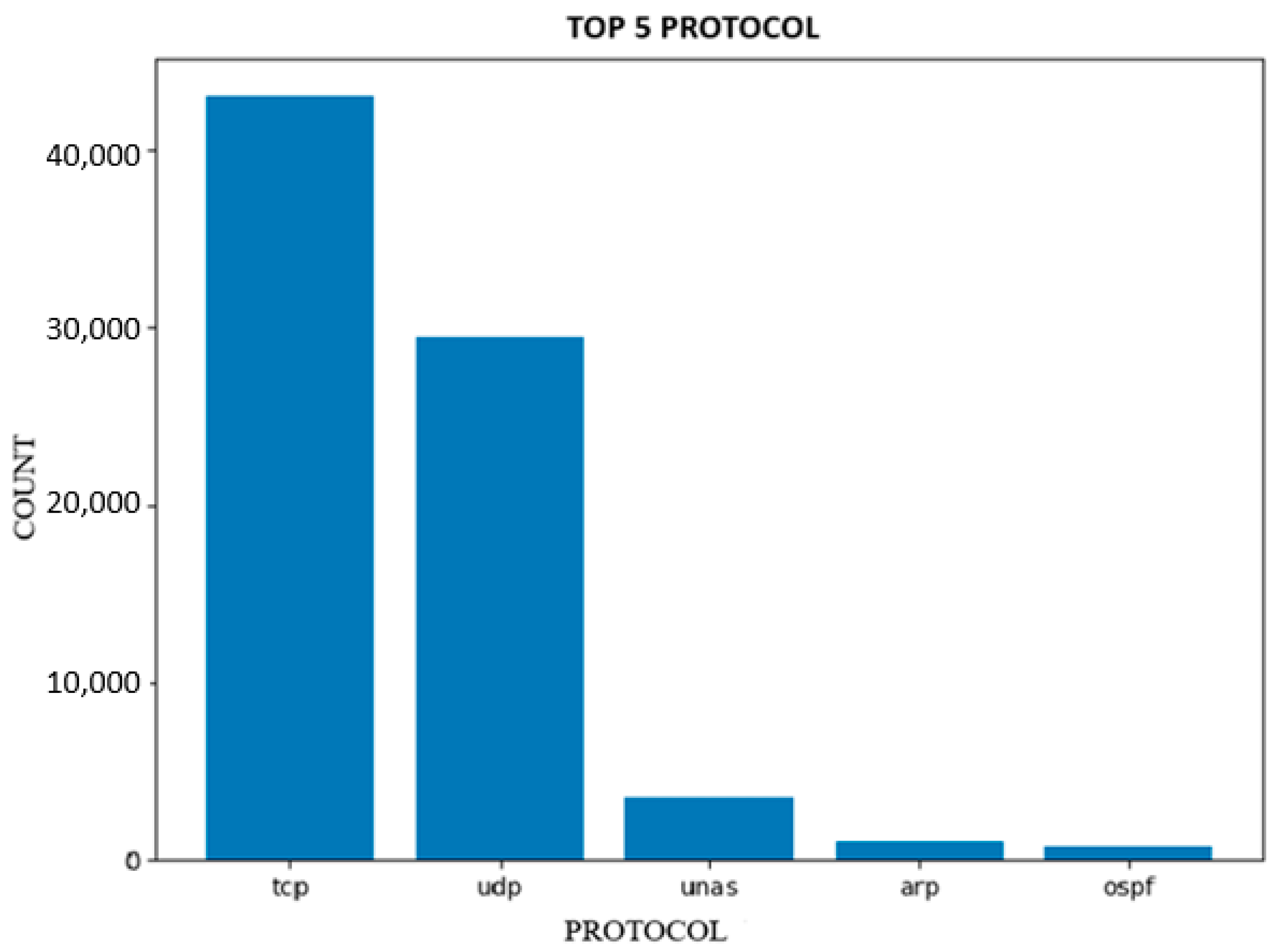
• Protocol Distribution: Determining the most often utilized protocols in IoT systems can be achieved by employing a visual representation such as a pie chart or bar plot, as shown in Figure 3 to showcase the distribution of these protocols throughout the dataset. It can facilitate the identification of protocols that are more susceptible to attacks and that require implementing supplementary security measures.

The term “protocol” pertains to a collection of regulations or criteria that dictate how data is conveyed and received across a network. In datasets related to network security, the column labeled “proto” commonly denotes the protocol employed for each network connection or packet, encompassing protocols like TCP, UDP, ICMP, and others. A comprehensive knowledge of the protocol used in network communication holds significant importance in network security applications, as distinct protocols may be susceptible to certain forms of attacks. There were many protocol types involved in this dataset, around 131, but we only visualized those with the maximum distribution in the dataset. TCP and UDP are the two most prevalent protocol types.

• Correlation Matrix: A correlation matrix can provide insights into the relationships between different properties within a dataset. Adopting this approach will facilitate a more comprehensive understanding of the critical attributes that hold the most significance in the anomaly identification process while distinguishing those that may be superfluous or lacking in substance. Below, Figure 4 shows the correlation matrix for selected features of the UNSW data frame.

Correlation is a robust descriptive measure that provides valuable insights into the degree of association between two variables. The strength of the association between variables can be assessed using the correlation coefficient. A correlation coefficient close to 1 indicates a high degree of correlation, whereas a value below 1 or negative suggests a weak relationship between the variables. In the figure above, only significant features were depicted, with those presented in blue hues indicating a strong correlation, while those shown in red hues denote a weak correlation. Additionally, the correlation coefficient is displayed on each correlated box, providing a quantifiable correlation assessment.

• Box Plots of Feature Distributions: The examination of box plots depicting the distributions of individual characteristics enables comprehension of the variability and distribution of the data. It can facilitate the identification of abnormal data points and outliers.

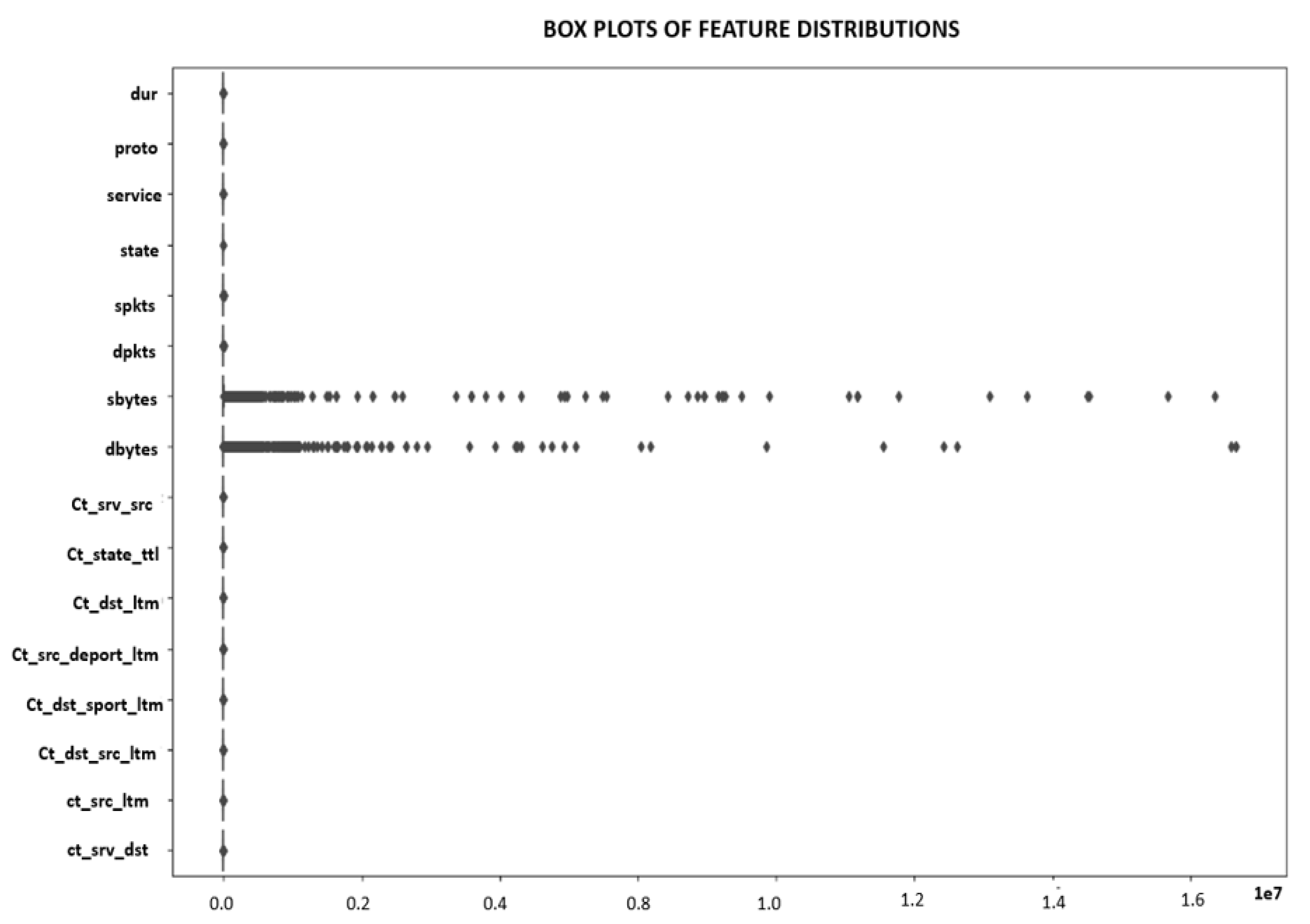
As depicted in Figure 5, outliers exhibit significant divergence from the remaining data points within the sample. The presence of outliers within the characteristics could indicate atypical or deviant patterns in the network traffic under investigation within the framework of this code. A significantly elevated value for the “sbytes” or “dbytes” attribute indicates the presence of huge network packets. Identifying and analyzing outliers can facilitate an understanding of network traffic patterns and the detection of anomalous behavior. Additional research may be necessary to ascertain the underlying source of any observed outliers, as outliers might arise from measurement errors or other factors unrelated to network traffic behavior.

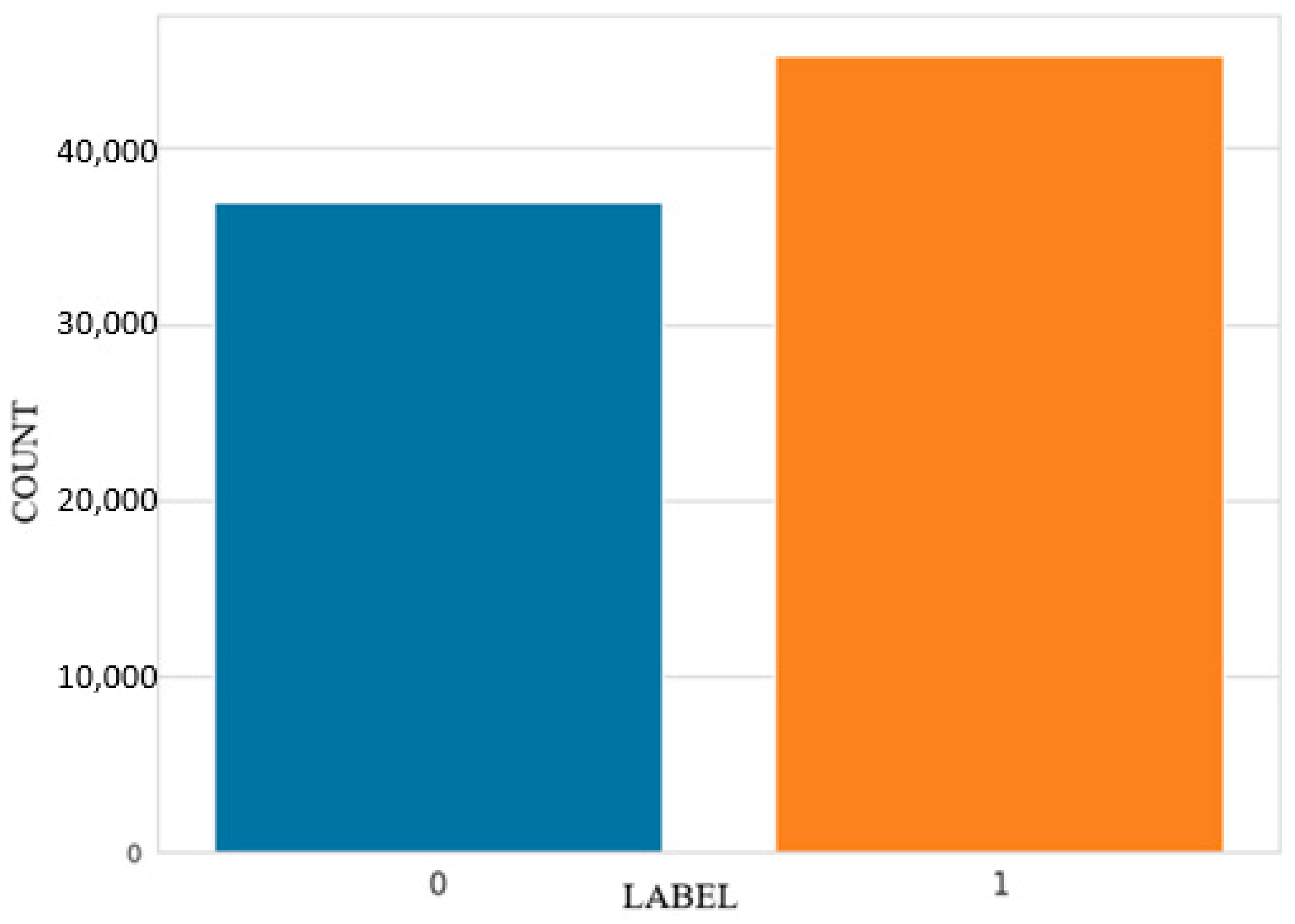
• Distribution of Label Classes: The equilibrium of the dataset can be ascertained by examining a bar plot that exhibits the distribution of the label classes, namely, normal or assault. Considering an imbalanced dataset is crucial when creating a machine learning model for anomaly detection.

The visualization presented in Figure 6 depicts the distribution of binary label classes, with 1 representing regular traffic and 0 representing harmful traffic. In contrast to a multi-label distribution characterized by significant class imbalance over ten classes, the label distribution under consideration exhibits balance. Consequently, it may serve as a promising target variable for developing a prediction model focused on anomaly identification.

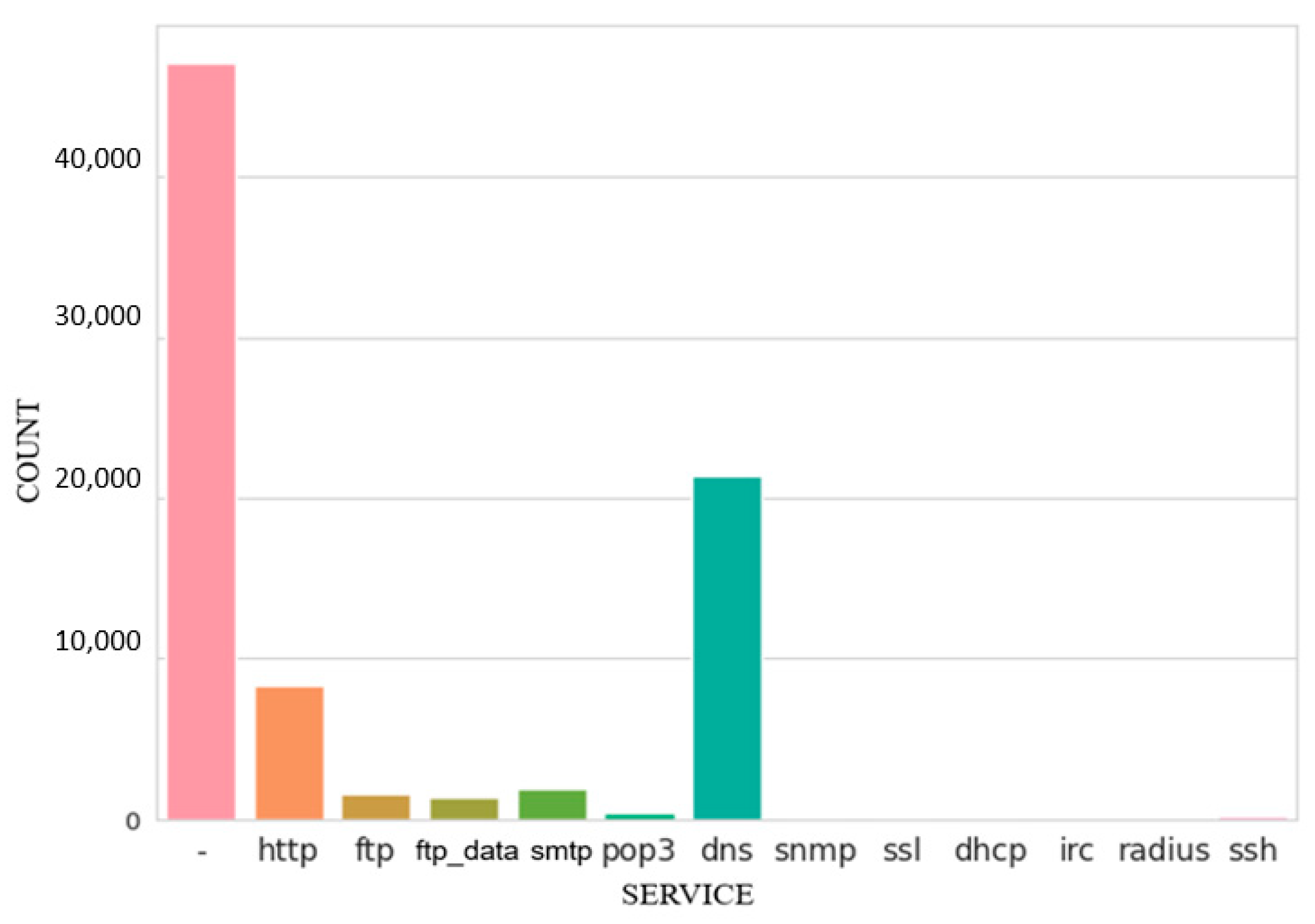
• Service Distribution: Figure 7, titled “Service Distribution Count,” depicts the frequency of various service types utilized in the dataset. The graph serves as a tool for discerning commonly employed network traffic services that may be susceptible to security breaches.

The chart’s vertical axis represents the quantity of each service, while the horizontal axis enumerates the many types of services. To facilitate the identification of the most commonly utilized services, the bars in the chart depicting the frequency of each service are organized in descending order. This visual representation may aid network administrators in prioritizing the protection of commonly utilized services and implementing measures to defend them against potential vulnerabilities. The dataset indicates that DNS and HTTP are the most commonly utilized services.

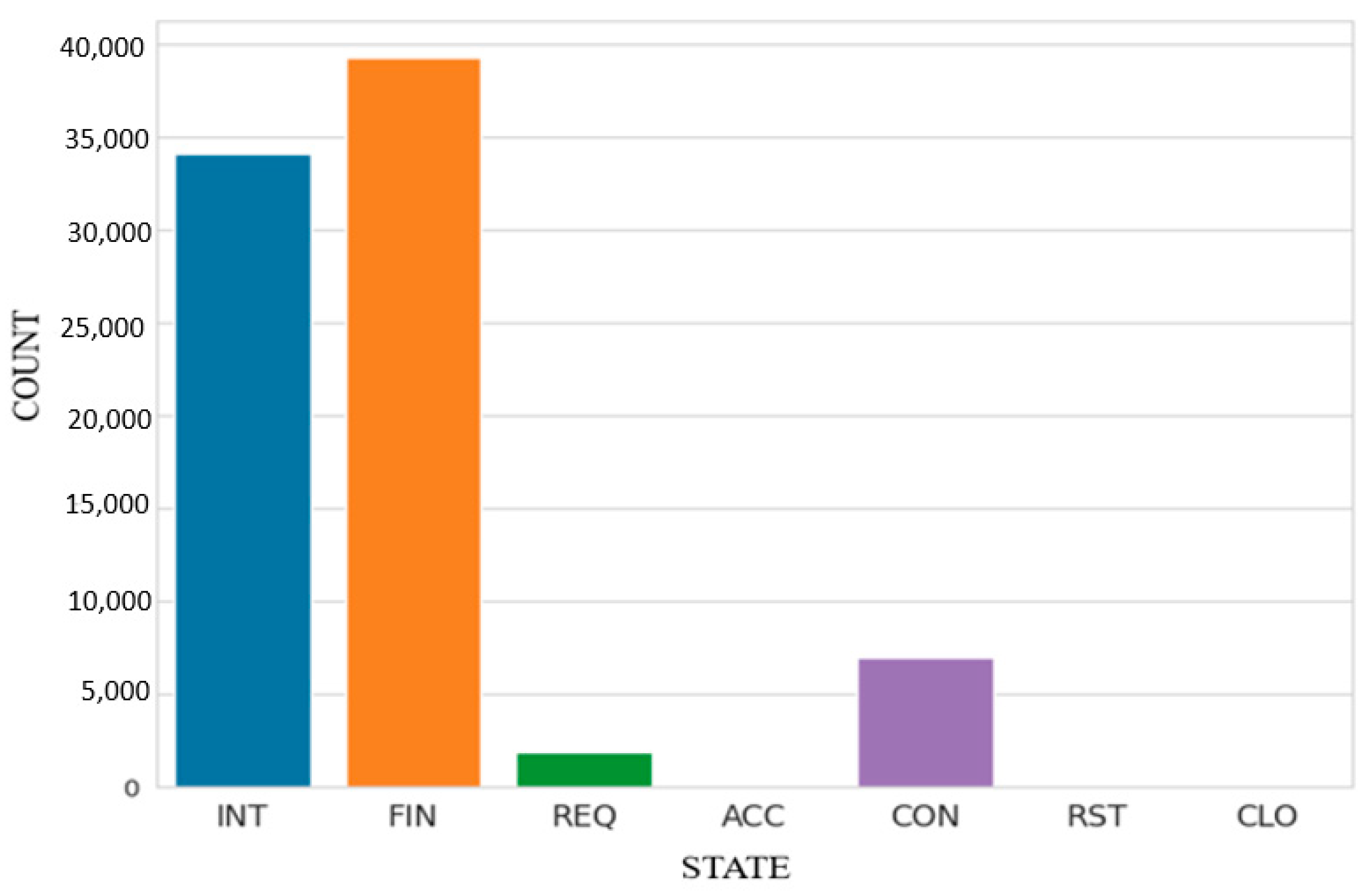
• State Distribution: The state distribution of a dataset characterizes the various states that a network connection may encounter over its lifespan. Established, Syn_sent, Fin_Wait1, Fin_Wait2, Time_Wait, Close, and other states are illustrative of such conditions.

Figure 8 displays the distribution of state types. Examining the distribution of states can offer valuable insights into the dynamics of a network and the characteristics of the traffic inside the dataset. Through the examination of state distributions, it becomes possible to discern potential anomalies and correlations that may exist between particular states and the various categories of attacks. Utilizing this knowledge can confer benefits in the advancement of ML models for anomaly detection, as well as the design of network security strategies.

3.3. Data Processing

The protocol for conducting data processing utilizing the UNSW-NB15 dataset for anomaly detection in IoT systems through active learning involves the following steps:

• Data cleaning: The data cleaning process includes identifying and removing duplicate records and the appropriate treatment of missing or erroneous data entries. It is possible to employ techniques such as one-hot or label encoding to convert categorical data into numerical form. The dataset under consideration exhibits a complete absence of missing or null elements. To complete the data cleaning process, it is necessary to convert the categorical variables in the dataset using label encoding. The dataset’s categorical variables, namely protocol, state, service, and attack_category, are presented in

  Table 3. Categorical variables.

  Proto	State	Service	Attack_Cat
  UDP	INT	-	Normal
  UDP	INT	-	Normal
  UDP	INT	-	Normal
  UDP	INT	-	Normal
  UDP	INT	-	Normal

  .

Upon the use of label encoding, the categorical variables are transformed into numerical representations, denoted by the values 0, 1, 2, 3, and so on. This conversion is illustrated in

Table 4. Label encoded categorical variables.

Proto	State	Service	Attack_Cat
117	4	0	6
117	4	0	6
117	4	0	6
117	4	0	6 0
117	4	0	6

.

• Feature Selection: Choose the characteristics that have the utmost significance in identifying abnormalities. Consider the concept of domain competence and the importance of feature significance metrics such as mutual information and correlation. To enhance the outcomes, it is possible to select specific traits that exhibit a strong correlation. However, previous studies have predominantly employed a limited number of characteristics. This study aims to construct an anomaly detection model using all available data, encompassing highly and minimally linked features.
• Feature Scaling: To ensure comparability, it is necessary to standardize the scales of the features. Standardization and min-max scaling are widely used techniques in data pre-processing. To ensure consistency within our dataset, we utilized traditional scalar operations. The revised data frame is presented in

  Table 5. Standardized features data frame.

  0	1	2	3	4	5	6
  1.457197	−0.110851	0.088625	−0.674406	−2.050741	−0.094586	−0.134511
  −1.176180	−0.213728	0.410563	0.274329	0.932695	−0.124455	−0.151816
  0.569545	−0.213729	−3.881935	−0.674406	0.932695	−0.124455	−0.151816
  −0.081899	−0.206895	0.088625	−0.674406	−0.559023	0.204110	0.263504
  −0.035069	−0.090130	0.088625	−0.674406	−0.559023	−0.064716	−0.099901

  .
• Train/Test Split: Generate training and testing datasets by partitioning the available data. The testing set will be utilized to evaluate the efficacy of the anomaly detection model after its training on the training set. The data frame consisting of 45 columns will be initially partitioned into two separate frames:

  ○

  1: Qualities.

  ○

  2: Education.

The initial 43 feature variables will be included in the features data frame. Two variables are used to represent the classes in our study: one is binary, while the other is multi-dimensional. In the present investigation, we will exclude the multi-label target variable and solely focus on binary labels. Subsequently, the dataset will be partitioned into a training set including 70% of the data and a testing set comprising the remaining 30%, using Sklearn’s train–test split procedure.

• X_train size = (57,632, 43)
• y_train size = (57,632)
• X_test size = (24,700, 43)
• y_test size = (24,700)

The initial record consists of many rows, while the subsequent record has multiple variables within each data frame. The training and testing feature sets comprise 43 variables, while the training and testing classes or target sets consist of 1 variable.

• Active Learning: To train the model, selecting a small subset of labeled data is recommended. The selection of the most informative data points can be iteratively performed using an active learning approach, wherein a human expert or a trained classifier is involved in the labeling. Incorporate the designated data points into the training set and afterwards engage in iterative model retraining to achieve the required level of performance.
• Evaluation: Analyze the model’s performance on the test set. Various metrics, such as accuracy, recall, F1-score, and Area Under the Curve Receiver Operating Characteristics (AUC-ROC), can be employed to assess the efficacy of abnormality detection.

4. Proposed Methodology

The approach that is suggested in our research focuses on an active learning framework for an IoT anomaly detection system. A machine learning technique called active learning reduces the need for labeled data while increasing model accuracy. It operates by actively choosing particular data points for labeling, decreasing the cost of annotation, and improving accuracy by emphasizing instructive samples. To more accurately discover anomalies with fewer labeled data points, active learning quickly locates and categorizes anomalous data inside complex IoT datasets. 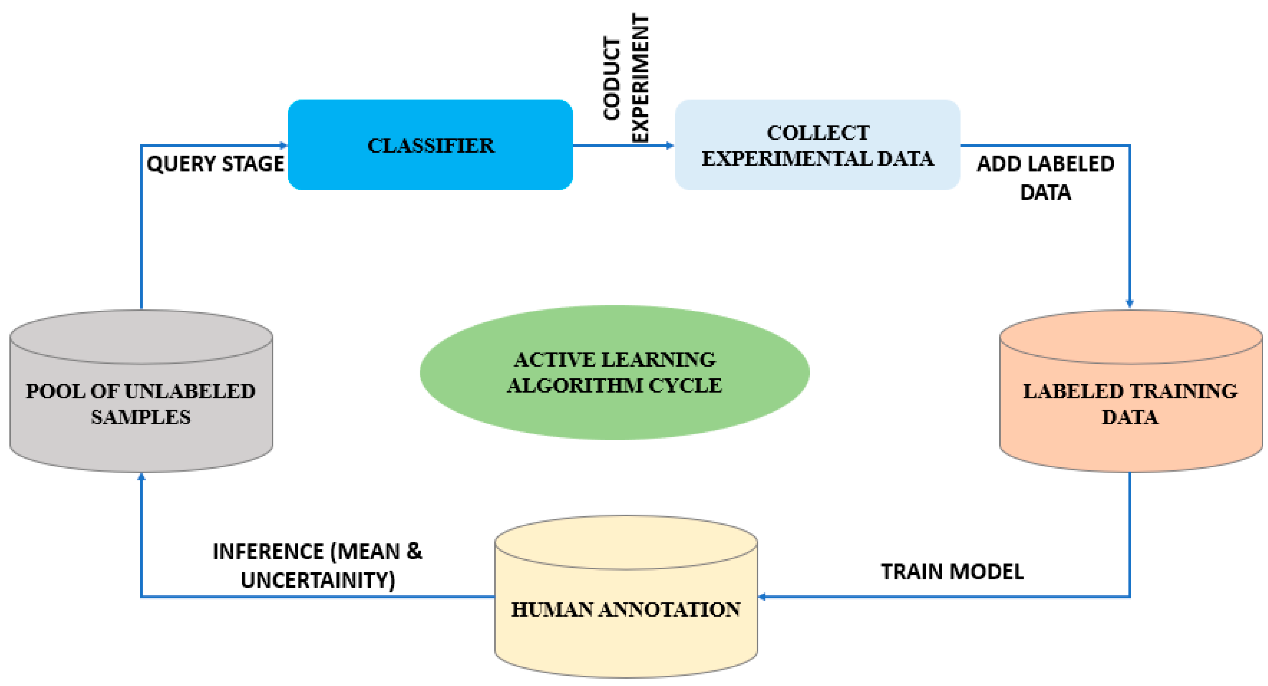Figure 9 shows our active learning system, which blends supervised and unsupervised techniques to improve anomaly detection. While the unsupervised portion locates potential anomaly clusters, the supervised portion categorizes the data as normal or anomalous. Active learning adapts to different IoT data types and applications by iteratively classifying data based on uncertainty. Entropy and information theory constitute the basis of active learning, particularly uncertainty sampling. A probability distribution’s entropy measures its degree of randomness, and active learning chooses which data to label by maximizing information gain. Entropy-based uncertainty sampling, which concentrates on data points close to the decision border or those where the model is uncertain, is the fundamental basis of active learning. Entropy, margin, and variance are three metrics that help it choose data points. Our model uses the modAL package for autonomous active learning and a random forest classifier. The model finds ambiguous instances in the test set, labels them, and adds them to the training set at the end of each iteration. It is especially helpful in situations when there is little or expensive labeled data since it minimizes labeled data while optimizing accuracy. This procedure continues until a performance threshold is reached.

4.1. Active Learning

Active learning is a machine learning strategy that aims to enhance the accuracy of a model with a reduced number of labeled data points. In this approach, the computer actively selects the specific data points to be marked. Additionally, active learning is a strategy that reduces the expense of annotation and enhances accuracy by choosing the most informative samples for human annotation repetitively, hence requiring fewer labeled examples. Active learning can be employed as a rapid approach to identify and classify atypical data points within a large and intricate dataset to find anomalies in IoT systems. The active learning algorithm selects the most informative data points for labeling by focusing on areas of the dataset where anomalies are anticipated to arise. This approach has the potential to significantly reduce the number of labeled data points needed to achieve the accurate detection of abnormalities. The general architecture of active learning is depicted in Figure 9 above.

The revised depiction in the experimental environment for the suggested approach, as depicted in Figure 9, offers a thorough representation of the active learning algorithm. The understanding of the query stage is heightened, as it is a crucial element within the active learning process. The classifier is provided with a pool of unlabeled examples during the query step. This stage is of significant importance as it entails the intentional selection of valuable data points from the dataset lacking labels to assign labels to them. By strategically selecting the most valuable samples, we enhance the algorithm’s efficiency and efficacy in acquiring knowledge from a restricted set of labelled data. Incorporating the testbed experiment within the image constitutes a noteworthy supplementary inclusion. The testbed experiment constitutes a crucial stage in assessing the performance and efficacy of the algorithm under consideration. The process entails gathering empirical data to evaluate the algorithm’s performance inside predetermined parameters or situations. By presenting the testbed experiment in the picture, we underscore the empirical basis of our methodology and its practical relevance. In addition, the revised depiction integrates the procedure of assigning labels to the chosen samples. Labelling the selected samples entails the assignment of accurate and verified labels to the data points that have been specifically selected for annotation. This particular phase is of the utmost importance as it enables us to acquire labelled samples, which can enhance the training data. Including these labelled samples in the training dataset enhances the precision and dependability of the algorithm’s predictions when utilized on the remaining set of unlabeled samples. The revised depiction within the experimental platform for the suggested technique offers a more intricate and all-encompassing portrayal of the active learning algorithm. This statement emphasizes the significance of three key elements: the query stage, the incorporation of a testbed experiment, and the labelling of chosen samples. The comprehension of the active learning process and the efficacy of the proposed algorithm are augmented by the visualization of these crucial steps.

4.2. The Foundational Mathematical Equations for Active Learning

Active learning is a machine learning methodology that involves identifying and selecting data points that possess significant informational value for expert labeling. The primary objective of active learning is to minimize the quantity of labeled data required to attain a specific performance threshold.

On the other hand, uncertainty sampling draws upon the principles of information theory, while the notion of entropy forms the foundational mathematical framework for active learning. The measure of entropy in a probability distribution signifies the degree of randomness or uncertainty present within it. In the context of active learning, the selection of data points for labeling is determined by assessing the entropy of a model’s output to identify the most informative points.

Let us define these terms:

• X is a collection of all potential input data items.
• Y is a collection of all potential output labels.
• D is the labeled training set of data.
• U is the group of all unlabeled data points.
• H is a collection of all conceivable hypotheses (models).
• The primary goal of active learning is to select a subset of the universal set U, denoted as the query set Q, to obtain expert annotations. The approach utilizes the entropy of the model’s output to ascertain the anticipated information gain for each data point within the set Q.

For a particular data point x, the model’s output entropy is defined as

$$H (\left(Y|x,D\right)=-\sum \left(y|x, D\right){\log }_p\left(y|x, D\right)$$

(1)

where, given the input data point x and labeled data D, $p \left(y\right|x, D)$ is the posterior probability distribution across the output labels.

For a data point x, the anticipated information gain is specified as follows:

$$IG \left(x, D\right)=H\left(Y|D\right)-E\left[H\left(\left(Y|x, D\right)\right)\right]$$

(2)

where $E [H (Y|x, D)]$ is the anticipated entropy of the output labels for x given the present model and the labeled data, and H(Y|D) is the entropy of the output labels for the entire dataset.

The algorithm selects the data points that exhibit the highest anticipated information gain to augment the labeled dataset D. The process is iterated until the desired level of performance is achieved, at which point the model undergoes retraining using a newly labeled dataset. To achieve a specific group level of performance with minimal labeled data, active learning utilizes the concept of entropy to select the most valuable data points for annotation. Algorithm 1 illustrates the procedural phases of the uncertainty sampling technique.

Algorithm 1: Uncertainty Sampling

4.3. Uncertainty Sampling

A popular method in active learning for determining which data points to identify as the most useful is the uncertainty sampling algorithm. The method seeks to utilize the labeling budget as effectively as possible by considering uncertainty. The steps of the uncertainty sampling algorithm will be covered in this part, along with information on how it is implemented in code. Finding the K data samples with the highest uncertainty ratings is the first step in the uncertainty sampling algorithm. These evaluations are based on how confidently each data point was predicted by the model. The sample is thought to be more valuable for annotation the greater the uncertainty rating. The program then requests accurate labels for each of the K unsure samples and adds them to the labeled dataset D when the K uncertain samples have been discovered. Then, using the newly labeled samples, a new model is trained on the updated dataset D. Iteratively, this process goes on until the labeling budget is depleted or the desired target performance is attained.

The main goal of the uncertainty sampling algorithm is to choose data points that will maximize the expected information gain. The algorithm attempts to decrease the uncertainty of the model’s predictions and increase the accuracy of those predictions by actively seeking the most uncertain data. Through a series of iterations that involve selective annotation and model retraining, the performance of the model with sparsely labeled data is gradually improved. The uncertainty sampling algorithm uses the idea of entropy to quantify uncertainty in its implementation. A probability distribution’s entropy measures the degree of randomness or uncertainty it contains. In order to lower the total uncertainty of the model’s predictions, the algorithm chooses data points. Calculating the uncertainty score for each data point is part of the code for the uncertainty sampling algorithm. The estimated probabilities of the model for each class label can be used to obtain this score. The K samples chosen for annotation are those with the greatest scores for ambiguity. The labeled dataset is used to train the model, and the procedure is repeated until either the required performance level is reached or the budget is used up. The uncertainty sampling algorithm, which chooses data points based on their expected information gain, is an efficient method for active learning. The approach seeks to increase classification accuracy with less labeled data by iteratively annotating the most ambiguous examples and retraining the model. The method effectively makes use of the labeling budget that is available by incorporating the idea of entropy to improve the performance of the model.

• Define the function of the uncertainty score:

US (x) = 1 − P (max∣x, D)

(3)

Given the input x and the current dataset D, y_max is the label with the highest probability. The chance that the label y_max will appear given the input x and the current dataset D is known as P (y_max|x, D).

2.

Select the K samples with the highest ratings for uncertainty.

Sk = {x_i} i = 1k where x_i = argmax x ∈ U US(x)

(4)

where U is the collection of data points without labels.

3.

Ask for the accurate label for each sample in S_k, then include them in the labeled dataset D.

4.

Train a new model on the revised dataset D, then continue the procedure until the budget is used up or the target performance is attained.

The concept of uncertainty sampling, which evaluates the uncertainty of a model using many measurements, serves as the foundational mathematical principle behind active learning. Entropy is a statistic that quantifies the amount of information required to classify a given piece of data accurately. Entropy-based uncertainty sampling selects the data points close to the decision boundary or those for which the model exhibits the least certainty in their classification. The formula for entropy-based uncertainty sampling is as follows:

$$x\_i=argmax\_x \sum ^C\_j=1 (-p\_ij log(p\_ij\left)\right)$$

(5)

where p_ij is the anticipated probability of class j for data point x_i, C is the number of classes, and x_i is the data point with the maximum entropy.

Another statistic to consider is the margin, representing the difference between the two highest projected probabilities. Margin-based uncertainty sampling is employed to select data points that exhibit the smallest discrepancy between the two highest projected probabilities. The formula for margin-based uncertainty sampling is as follows:

$$x\_i=argmax\_x min\_j\in \{1,\dots ,C\},j\ne y\_i (p\_ij-p\_iy\_i)$$

(6)

where x_i is the data point with the lowest margin, C is the number of classes, y_i is the accurate class label for data point x_i, and p_ij is the estimated likelihood that class j will occur for data point x_i.

Variance, which refers to the degree of fluctuation in the model’s predictions, constitutes a third metric. Variance-based uncertainty sampling is employed to select the data points that exhibit the most significant variability in the model’s predictions. The mathematical expression for uncertainty sampling, which is determined by variance, can be represented by the following formula:

$$x\_i=argmax\_x (1/T) \sum ^T\_t=1 (p\_it-(1/T) \sum ^T\_t\prime =1 p\_it\prime )^2$$

(7)

where T is the total number of model predictions, p_it is the projected probability of class j for data point x_i in the t-th model prediction, and x_i is the data point with the highest variance.

Active learning can attain superior model performance using a reduced number of labeled data points by selecting the most valuable data points for labeling. This approach is particularly advantageous when obtaining labeled data is challenging or costly.

The active learning process involves training a model iteratively on a limited portion of the available data, referred to as the active learning set. This trained model is then utilized to select the next set of data points that require labeling, which is subsequently added to the active learning set. The procedure above is commonly referred to as active learning. The process above continues iteratively until the desired level of precision is achieved, or a predetermined stopping criterion is met. To reduce the amount of labeled data required for training and to enhance the model’s accuracy, active learning endeavors to select the most informative and representative data points for annotation.

4.4. The Architectural Framework of an IOT-Based Smart City

The operational environment of a smart city can be seen to incorporate technology like the Internet of Things and other intelligent systems. This connection makes it easier for information to flow freely and helps with the efficient administration of different services. The wide variety of technologies present in a smart city contributes significantly to the improvement of several industries, such as energy consumption, healthcare, education, logistics, and pollution reduction. Three separate layers make up the architectural composition of a smart city: the fog layer, the cloud layer, and the terminal layer, in that order.

The storage resources, which include servers and other devices that facilitate the processing and management of large amounts of data, are included in the cloud layer. The fog layer is the term used to describe the intermediate layer that creates a link between the cloud layer and the terminal layer. Data flow between sensors and Internet of Things devices is facilitated by the terminal layer’s interactions with a variety of devices. It also gathers data that is both structured and unstructured. Figure 10 illustrates the IoT-based smart city’s architectural foundation.

4.5. Model Architecture Design

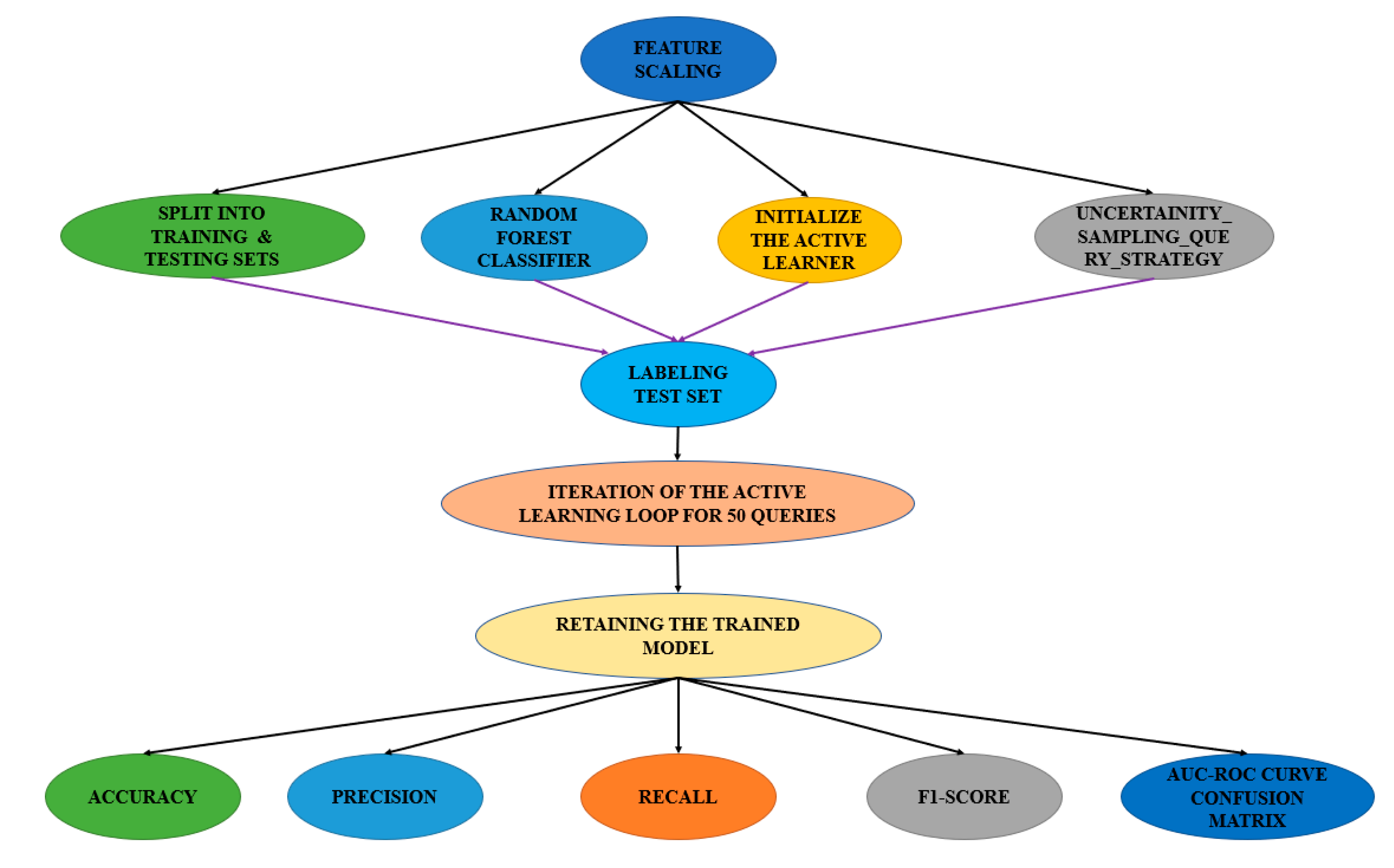
The method under consideration employs a random forest classifier sourced from the Scikit-Learn toolkit as its primary constituent. The classifier comprises a collection of 50 decision trees, each with a depth of 15. The random forest classifier utilizes ensemble learning to perform classification and regression tasks. The algorithm constructs a set of decision trees and afterwards calculates the class or average prediction by combining the outputs of these trees. The ultimate forecast of the random forest model is derived from a majority vote among the individual trees that have been trained on a subset of randomly chosen features. Furthermore, the input features undergo pre-processing and normalization through the utilization of the StandardScaler approach. As shown in Figure 11.

The modAL package is utilized for the implementation of active learning. This enables the model to independently determine the data samples that require labelling in each iteration, in contrast to labelling all the data samples simultaneously, as is customary in traditional techniques. The ActiveLearner class within the MODAL framework is employed for this specific objective. During the initialization phase, the necessary components for the experiment are configured, including the training data, the random forest classifier as the chosen estimator, and the uncertainty_sampling query technique. The query approach known as uncertainty sampling is responsible for selecting examples that the model exhibits the least certainty in classifying. The implementation of this technique utilizes the uncertainty_sampling function provided by the modAL library. The uncertainty sampling approach is employed to choose data points by considering the model’s highest level of uncertainty in its predictions. This level of uncertainty is determined by subtracting one from the likelihood of the label that is most likely to be correct. During each iteration of the active learning loop, the model selects the instances with the highest level of ambiguity from the test set, assigns labels to these instances, and subsequently integrates them into the training set. The procedure is iterated for a predetermined number of inquiries, specifically 50. Following each query, the model is subjected to retraining using the adjusted training data, followed by the computation of accuracy using the test data. The correctness of every iteration is documented, and the cumulative accuracy is stored as the variable “acc”. The algorithm incorporates an active learning framework to efficiently identify anomalies in the Internet of Things (IoT) domain. This is achieved by harnessing the capabilities of random forest classification, uncertainty sampling, and an iterative approach for selecting and labelling cases that exhibit ambiguity. The provided description offers a thorough understanding of the operational mechanism of the algorithm under consideration.

4.6. Model Training

The implementation of active learning improved our model’s performance, achieving a remarkable accuracy of 99.7%. This outcome can be attributed to a range of potential factors. One possible explanation could be that active learning facilitates the expert’s ability to select the most informative data points for annotation, enhancing their efficiency in utilizing their time and resources. Active learning can reduce the required number of samples for achieving high accuracy by focusing on the most informative occurrences. It can be particularly advantageous in large datasets where identifying all samples may prove unfeasible or cost-prohibitive.

A further factor to consider is that implementing active learning techniques can mitigate the challenge of class imbalance, a common issue seen in occupations requiring anomaly identification. Implementing active learning techniques has been shown to enhance the classifier’s ability to detect anomalies and reduce the occurrence of false positives. It is achieved by strategically selecting samples from the minority class that provide difficulties in classification. Active learning can potentially improve the performance of anomaly detection models by choosing the most informative samples for labeling and addressing the class imbalance problem.

5. Results

Model assessment is a pivotal stage in machine learning since it evaluates the performance of a trained model on novel and unexplored data. The subsequent list of the customary evaluation metrics can be used for anomaly identification.

• Precision

Precision refers to the proportion of accurate optimistic predictions made by a model that are true positives, meaning it correctly identifies anomalies. A model with a high accuracy score suggests a minimal occurrence of false positives.

• Recall

The true positive rate is the percentage of real anomalies in the dataset that were found. A model with few false negatives has good recall accuracy.

Table 6. Evaluation metrics of the proposed model.

Evaluation Metric	Performance Value
Weighted Average Accuracy	0.995
Accuracy	0.997
Precision	0.974
Recall	0.971
F1-Score	0.992

presents the evaluation metrics pertaining to our suggested model.

• F1-Score

These are two requirements balanced by the harmonic mean of accuracy and recall. A well-balanced model with great accuracy and recall has a high F1-score.

• Receiver Operating Characteristic (ROC) Curve

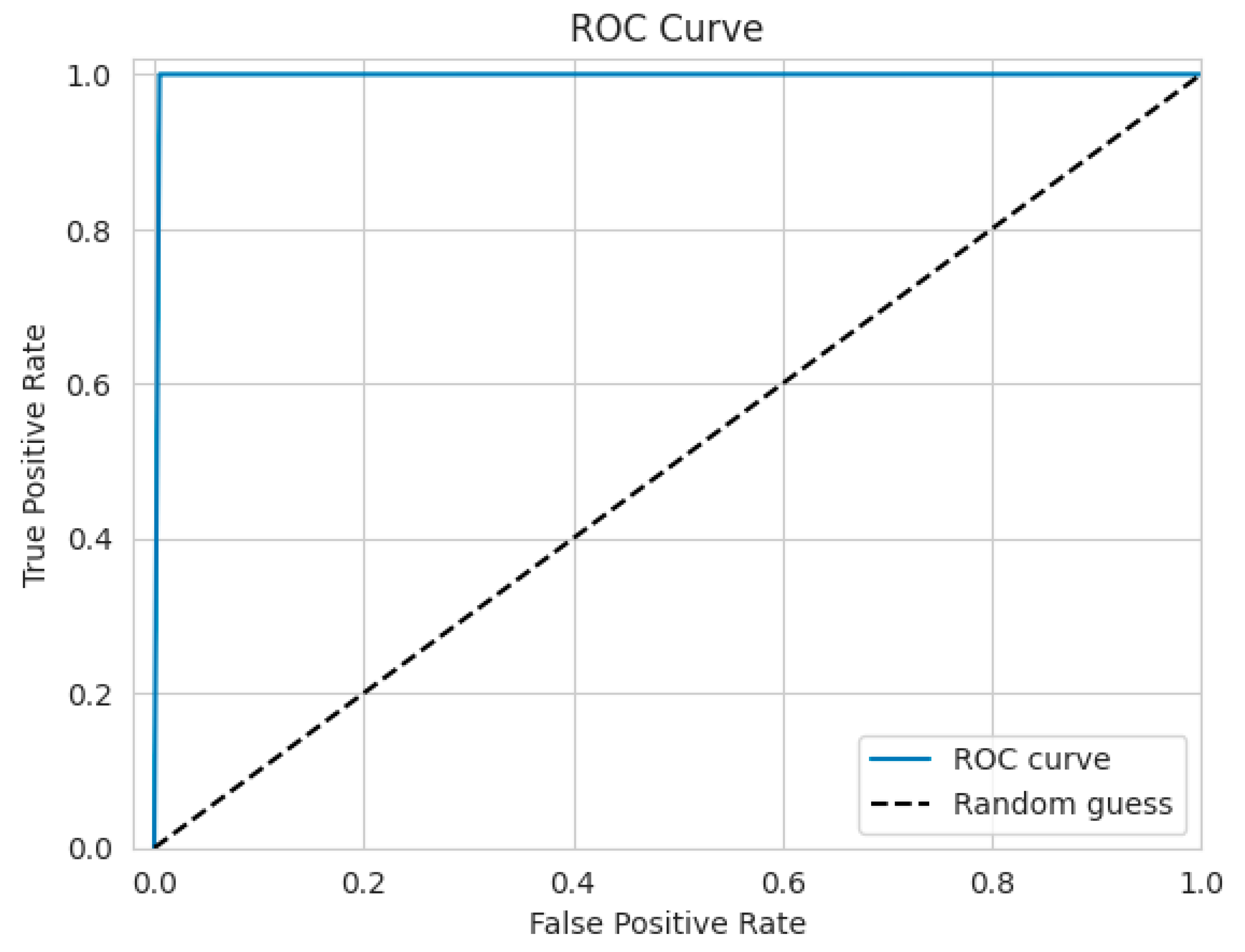
Image 13 shows the relationship between the genuine positive rate (recall) and false positive rate (1-specificity) at different thresholds. This illustration is frequently referred to as a ROC curve. One measure used to evaluate a model’s overall performance is the AUC score. A rating of 1 signifies optimal categorization performance, whereas a score of 0.5 denotes random guessing.

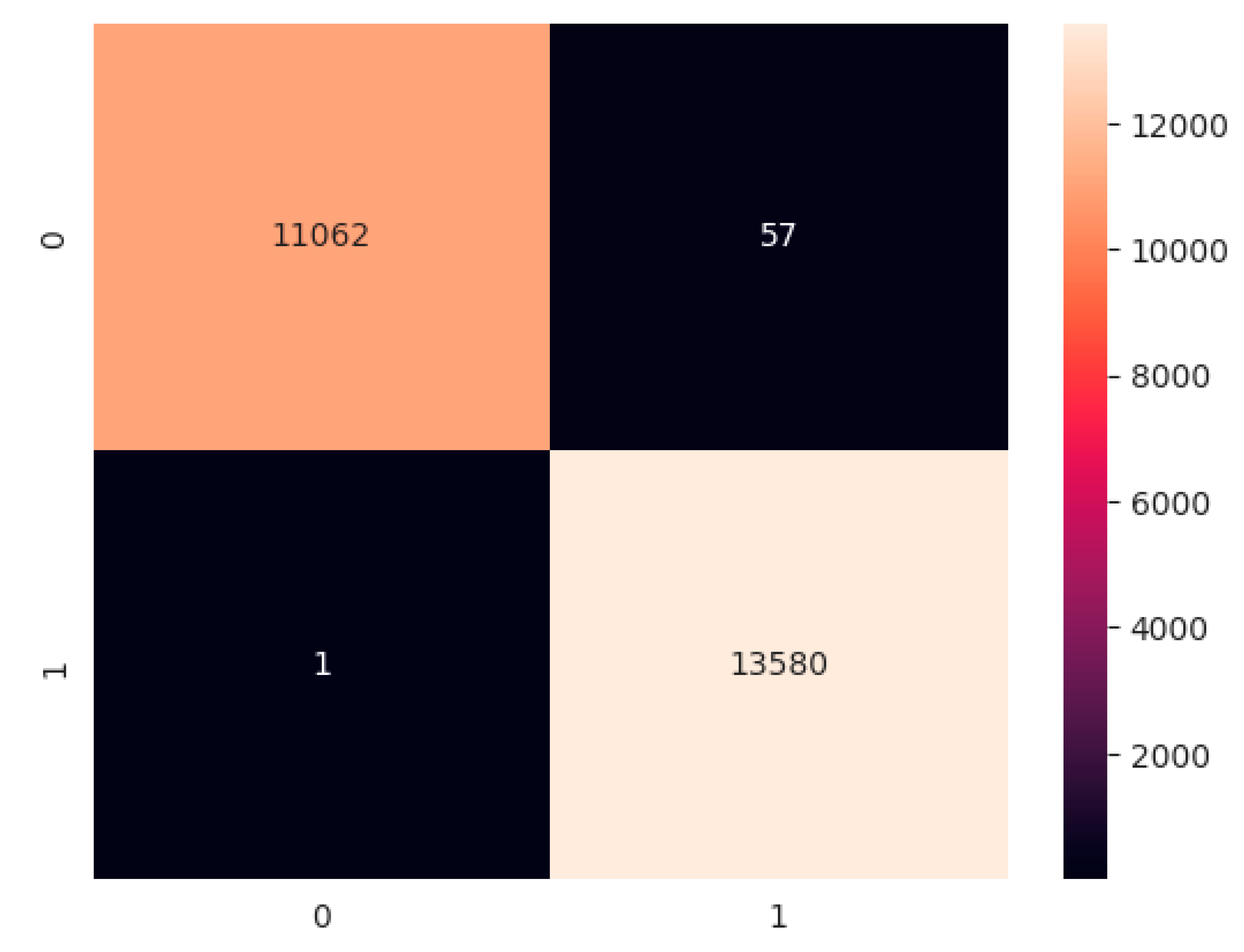
5.1. Confusion Matrix

A confusion matrix simplifies the machine learning system evaluation. Model performance is measured by correct predictions, including true positives, true negatives, false positives, and false negatives. True positive (TP) models effectively anticipate the positive class. A true negative (TN) occurs when the model properly predicts the negative class. A model FP happens when it mis-predicts the positive class. A false negative (FN) occurs when the model mis-predicts the negative class.

Figure 12 below illustrates that 11,062 samples from the test data were accurately predicted within the harmful class, whereas 57 samples were incorrectly classified as belonging to the normal class. In the normal class, a total of 13,580 instances were accurately predicted, with only one instance being incorrectly predicted. The discrepancy in incorrect predictions between the two classes can be attributed to a slight imbalance within the dataset, wherein the number of normal samples exceeded that of malicious samples.

In assessing the effectiveness of an anomaly detection model through active learning, it is essential to monitor the number of labeled instances employed for training during each iteration alongside the progression of the performance metrics. Cross-validation techniques are additionally recommended to offer a more precise assessment of the model’s performance. When analyzing the mistakes generated by a model, it is crucial to consider many factors that may contribute to misclassification, including data imbalance, noise in the data, and model complexity.

The suggested model’s evaluation metrics are summarized in Table 6, which is an important part of evaluating the model’s performance. These metrics provide insightful information about the model’s effectiveness in several areas. With a high value of 0.995, the weighted average accuracy shows that the model is generally accurate in its predictions, even when the classes are unbalanced. The accuracy demonstrates that nearly 99.7% of the dataset’s cases are properly predicted by the model. It is an easy way to gauge overall accuracy. Another crucial statistic is precision, which now stands at 0.974. The proportion of accurate positive predictions made by the model is indicated by precision. This indicates that roughly 97.4% of the model’s optimistic predictions were correct. Recall is 0.971, which indicates that 97.1% of all real positive cases are captured by the model. The F1-score is currently 0.992. This measurement strikes a compromise between recall and precision. It shows that the model is achieving excellent results in balancing the reduction of false positives and false negatives. The performance of the suggested model, which is shown in the table, is encouraging. It exhibits high classification accuracy, strong classification precision, high recall, and high F1-score values, all of which indicate that the model is successful in properly classifying events in the dataset.

The receiver operating characteristic (ROC) curve illustrates the performance of prediction accuracy, as shown in Figure 13. A curve that approaches a value of 1 implies a strong version of the model. Conversely, a curve centered at 0.5 suggests that the model’s accuracy is approximately 50%. In our specific example, the curve is positioned at 1.0, indicating exceptional model performance with an accuracy close to 100%.

5.2. Novel Model Design

This study employed a fusion of active learning and machine learning techniques to identify anomalies in IoT systems. Active learning lowers the amount of labeled data needed to train an accurate model. This method selects and queries the most informative labeling data points iteratively. The model’s lowest certainty determines data points for labeling in this study’s uncertainty sampling active learning technique. A machine learning model was created using IoT device network traffic data. The researchers detected network intrusions using the freely available UNSW-NB15 dataset. Our work used a random forest classifier, an ensemble learning method that builds numerous decision trees and aggregates their predictions to improve model accuracy and robustness.

Initially, the dataset was partitioned into training and testing sets using an 80:20 ratio. The ActiveLearner object was initialized, encapsulating both the machine learning model and the active learning mechanism. To identify the most valuable data points for labeling, we implemented the uncertainty sampling methodology. A query limit of 50 was set, indicating that 50 data points from the test set would be selected for labeling. Throughout the active learning process, we utilized the ActiveLearner object to extract the most informative data points from the test set for labeling. The model was retrained after the incorporation of labeled data into the training set. Upon conducting calculations to determine the accuracy of the model after each query, it was observed that accuracy gradually improved as the active learning process advanced.

Ultimately, our approach exhibited superior performance to traditional machine learning techniques that do not incorporate active learning, with a test set accuracy of 99.7%. The primary advantage of our methodology lies in its ability to attain a high level of accuracy while utilizing a small quantity of labeled data. This characteristic is particularly valuable in the context of anomaly detection within the Internet of Things (IoT) systems, where the acquisition of labeled data might present challenges in terms of both feasibility and cost. Our innovative approach of integrating active learning with machine learning algorithms has the potential to enhance anomaly detection in IoT systems.

5.3. Core Contributions of this Study

The primary contributions of our study, titled “Anomaly Detection for IoT Systems Utilizing Active Learning”, are as follows:

• Development of an effective anomaly detection model using active learning: Our study has demonstrated that active learning is a valuable technique for developing precise and efficient anomaly detection models in IoT systems. The model can iteratively select the most informative data points by employing the uncertainty sampling technique. This approach enhances the model’s accuracy and decreases the requirement for a large number of labeled data points during the training process.
• Evaluation of the model on a real-world IoT dataset: Our model is evaluated on the UNSW-NB15 dataset, a publicly available dataset containing real network traffic data from an IoT device. The approach presented in this study demonstrates superior performance compared to various state-of-the-art anomaly detection techniques, with an accuracy rate of 99.7%.
• Investigation of the impact of different feature selection methods: This study examines how feature selection tactics affect our model’s performance. PCA, mutual information-based, and correlation-based feature selection are used to evaluate the model’s efficacy. Our analysis shows that reciprocal feature selection yields the greatest results.
• Identification of the most significant features for anomaly detection in IoT systems: Finding the most important features for IoT anomaly detection requires packet lengths, bytes sent, and packet send rates. Our research shows that these traits can detect unusual IoT traffic patterns.
• Demonstration of the potential of active learning for future IoT applications: This study suggests using active learning in Internet of Things applications. We recommend active learning for creating robust and effective anomaly detection models for Internet of Things applications in the near future. Active learning can substantially reduce the cost and time of constructing Internet of Things anomaly detection models. This is achieved by reducing the labeled data for training.

5.4. Comparative Analysis

The research conducted in our study, titled “Anomaly Detection for IoT Systems through the Application of Active Learning,” surpasses previous investigations by achieving a remarkable accuracy rate of 99.75% when evaluated on the UNSW-NB15 dataset (

Table 7. Recent work related to anomaly detection.

Reference	Approach	Accuracy	Dataset
[7]	SVM	92.6%	UNSW-NB15 dataset
[10]	SVM	90.50%	UNSW-NB15 dataset
[14]	VLSTM	96.7%	UNSW-NB15 dataset
[16]	RF	96%	UNSW-NB15 dataset
[22]	SVM	94.3%	UNSW-NB15 dataset
[24]	RF	98.67%	UNSW-NB15 dataset
Our approach	Active learning	99.75%	UNSW-NB15 dataset

). Our model’s utilization of active learning facilitated the dynamic selection of highly informative data points for labeling. This approach effectively minimized the requirement for a large number of labeled data during the training process while maintaining a high accuracy level. This approach becomes particularly advantageous in situations where the acquisition of annotated data is expensive and time-consuming, but still yields enhancements in the model’s performance.

This study employed the random forest classifier as the chosen model due to its proven effectiveness on the UNSW-NB15 dataset. The random forest classifier, an ensemble learning technique, uses many decision trees to enhance accuracy and mitigate the risk of overfitting. This approach can capture the intricate relationships between the various attributes and the desired outcome, resulting in a model that exhibits superior performance.

To find anomalies in IoT systems, earlier research used supervised learning techniques like SVM, RF, and VLSTM on the UNSW-NB15 dataset. The accuracy scores of the investigations ranged from 90.50% to 98.67%.

To optimize the performance of our model, our study employed a range of feature engineering techniques, including scaling and normalization of the dataset. Furthermore, in the context of active learning, our model used various query methods based on uncertainty, including least confidence, margin sampling, and entropy sampling. Utilizing several query techniques enabled our model to effectively examine data distribution and select the most informative examples for labeling. By employing feature engineering techniques, active learning methodologies, and a random forest classifier, a robust anomaly detection model for IoT devices was successfully developed, exhibiting high accuracy. Our methodology reduces the cost and time required for labeling while improving the model’s functionality. It renders itself a viable choice for practical implementations.

6. Discussion

The objective of this study is to investigate the utilization of active learning techniques for anomaly detection within IoT systems. The identification of irregularities holds significant importance in guaranteeing the security and dependability of IoT systems. Given the substantial amount of data generated by these systems, it is imperative to maintain consistent monitoring to identify any anomalous patterns or behaviors. The utilization of supervised learning algorithms is frequently employed in IoT systems for anomaly detection, as these techniques necessitate tagged data for training. Nevertheless, the process of categorizing data can be laborious and demanding in terms of resources, particularly when the quantity of irregular data is considerably smaller compared to the normal data. Active learning is a pedagogical approach that addresses this challenge by intentionally choosing the most useful examples from a collection of unlabeled data. These selected examples are subsequently provided to human annotators for identification. The implementation of active learning as a pedagogical approach offers advantages in mitigating the workload associated with labeling tasks while ensuring a sustained degree of precision in detection. The procedure entails the repetitive choice of cases that exhibit either uncertainty or instructional value.

The present study employed uncertainty sampling as an active learning technique to pick samples for labeling, considering their degree of uncertainty. The enhanced efficacy of our model can be ascribed to the incorporation of a random forest classifier. The random forest methodology is well known for its capacity to effectively handle datasets defined by a high number of variables and yield reliable outcomes. The incorporation of an ensemble of decision trees within the random forest technique was employed to mitigate the potential issue of overfitting and enhance the precision and reliability of predictions. Furthermore, the decision to impose a limitation on the maximum depth of each tree to a value of 15 was made to mitigate the problem of overfitting, while simultaneously striking a balance between the accuracy and interpretability of the model. The assessment of our model on the UNSW-NB15 dataset generated favorable outcomes, therefore supporting the efficacy of our methodology. The effectiveness of the model in detecting irregularities in IoT network traffic data was demonstrated by its high performance metrics. These metrics include a weighted average accuracy of 0.995, an accuracy of 0.997, precision of 0.974, recall of 0.971, and F1-score of 0.992. The integration of active learning into our anomaly detection model for IoT devices, together with the application of a random forest classifier, has resulted in notable enhancements in performance. Through the implementation of a rigorous sample selection process and harnessing the collaborative nature of the random forest methodology, our model demonstrated an exceptional level of accuracy, reaching a rate of 99.7%. The aforementioned findings underscore the effectiveness of active learning methodologies and their ability to augment the identification of abnormalities in IoT systems.

7. Conclusions

In conclusion, our active learning approach outperforms previous methods by accurately detecting anomalies in IoT systems. Additionally, the precision and recall measurements of our approach further validate its effectiveness in correctly identifying anomalies. One of the key contributions of our research is the development of a unique uncertainty-based sampling strategy. By selecting the most informative instances for labeling, we were able to significantly reduce the labeling costs associated with anomaly detection in IoT systems. This not only saves time and resources but also improves the overall performance of the model. Furthermore, our framework, which combines active learning with random forest ensemble classifiers, proved to be highly effective in identifying previously unnoticed anomalies. It demonstrates the robustness and adaptability of our approach, making it a valuable tool for protecting IoT devices from potential vulnerabilities. It is worth noting that our findings have broader implications beyond IoT systems. Furthermore, through the utilization of various methodologies and the UNSW-NB15 dataset, we were able to compare and evaluate the performance of different algorithms. Our approach, which incorporated active learning, outperformed all other methods with an impressive accuracy rate of 99.75%. This highlights the effectiveness of active learning in enhancing the identification of anomalies in IoT systems. The integration of active learning successfully addressed the challenge of limited annotated data in IoT systems, as it allowed for the identification and labeling of the most informative examples.

Exploring the scalability and effectiveness of active learning techniques in large-scale IoT environments is essential for future research. A fascinating area for further investigation is looking into how advanced anomaly detection algorithms can be combined with active learning to improve the security and dependability of IoT systems.