
Prediction of Wind Power with Machine Learning Models

Department of Electronic and Automation, Vocational School, Batman University, Batman 72100, Turkey
Appl. Sci. 2023, 13(20), 11455; https://doi.org/10.3390/app132011455
Submission received: 11 September 2023
/
Revised: 14 October 2023
/
Accepted: 17 October 2023
/
Published: 19 October 2023
(This article belongs to the Special Issue Application, Optimization and Architecture of Deep Learning Neural Network)
Abstract
:Wind power is a vital power grid component, and wind power forecasting represents a challenging task. In this study, a series of multiobjective predictive models were created utilising a range of cutting-edge machine learning (ML) methodologies, namely, artificial neural networks (ANNs), recurrent neural networks (RNNs), convolutional neural networks, and long short-term memory (LSTM) networks. In this study, two independent data sets were combined and used to predict wind power. The first data set contained internal values such as wind speed (m/s), wind direction (°), theoretical power (kW), and active power (kW). The second data set was external values that contained the meteorological data set, which can affect the wind power forecast. The k-nearest neighbours (kNN) algorithm completed the missing data in the data set. The results showed that the LSTM, RNN, CNN, and ANN algorithms were powerful in forecasting wind power. Furthermore, the performance of these models was evaluated by incorporating statistical indicators of performance deviation to demonstrate the efficacy of the employed methodology effectively. Moreover, the performance of these models was evaluated by incorporating statistical indicators of performance deviation, including the coefficient of determination (R2), root mean square error (RMSE), mean absolute error (MAE), and mean square error (MSE) metrics to effectively demonstrate the efficacy of the employed methodology. When the metrics are examined, it can be said that ANN, RNN, CNN, and LSTM methods effectively forecast wind power. However, it can be said that the LSTM model is more successful in estimating the wind power with an R2 value of 0.9574, MAE of 0.0209, MSE of 0.0038, and RMSE of 0.0614.
1. Introduction
Within the realm of renewable energy, wind power has emerged as a prominent contender, primarily due to its sustainable nature, lack of pollution, and minimal cost implications. However, the randomness of wind power generation challenges the power grid’s secure dispatch and stable operation. Hence, precise wind power forecasting significantly reduces grid dispatching costs and enhances system performance [1,2]. Various factors, including climate, seasons, and the intermittent nature of wind, make forecasting wind power complex [3]. Furthermore, the lack of predictive abilities in wind power systems that undergo substantial fluctuations may result in contradictions and pose significant obstacles for power systems. Therefore, the successful integration of wind power at a global level relies heavily on accurate wind power prediction. It is demonstrated that challenges such as insufficient regulation and reserve power, often linked to the variability and limited predictability of wind power, can only be comprehensively evaluated when considering the characteristics of the conventional generation system with which wind power is integrated [4,5].
Scientists worldwide have conducted numerous research efforts to realise wind power prediction by developing various models in recent years. Numerous researchers, e.g., Rahman et al. [6], Ray et al. [7], and Abdalla et al. [8], have undertaken significant investigations to develop refined software models that are intended to predict power generation via the utilisation of RES. Some researchers have found that the amount of variable data affects wind power forecasting performance [9,10]. Li and Mao [11] proposed a method that utilises two-day historical climate data and wind power data for training a back propagation neural network. This network is employed to predict ultra-short-term wind power in the next 4 h based on numerical weather forecasts. Ma et al. [12] discovered in their study on short-term generation forecasting in a microgrid that neural networks consistently exhibit high performance across seasons. Unlike other algorithms, this method is not influenced by temperature variations, showcasing its remarkable flexibility. Lahouar et al. [13] studied hour-ahead wind power forecasting. They observed that neural networks are sensitive to irrelevant data, with model performance decreasing as the number of features increases. Additionally, their research revealed that the performance of neural networks can be compromised if their numerous parameters are not adequately tuned. In a study referenced in [14], a probability forecasting model for ultra short-term wind power was developed using a CNN. The accuracy of this model was subsequently evaluated to assess its performance. In [5], CNN and a physical model were integrated to enhance the accuracy of short-term wind power forecasting, significantly reducing forecasting errors. In [15], LSTM models have been utilised in short-term wind speed and power forecasting. Solas et al. [16] put forward a concise approach for wind power prediction, which relies on a CNN. Their findings revealed that this method outperforms ARIMA and Gradient Supercharger regarding wind power forecasting accuracy. Liu and colleagues [17] posited an innovative methodology for short-term wind power forecasting that leverages image representations of temporal data and applies CNN architectures for analysis. Comparative analyses with current approaches in wind power prediction, namely, RNN, LSTM, and GRU, exhibit the superior performance of the proposed method.
ANN-based forecasting enables rapid wind farm output power prediction despite the potential for significant output power disparities amongst individual wind generators resulting from inconsistencies in wind speed at each turbine [18]. Deep learning (DL) models offer a more robust computational capability and are better equipped to handle complex functions than shallow ML approaches. Using multi-layered network structures and nonlinear optimisation techniques, DL models could automatically extract meaningful features from data at various levels of abstraction, from low-level to high-level representations [19]. Several scientists endeavour to employ DL models in wind power prediction using past data to enhance the precision of wind power forecasting [20,21,22]. Recently, there has been an extensive exploration into the realm of DL, focusing on its implementation in short-term wind power prediction [13]. LSTM and CNN are recognised as the two primary DL models [23]. Existing individual CNN and LSTM models can establish nonlinear correlations between output and input variables by utilising large amounts of historical data. This enables accurate predictions of wind speed or wind power [24]. These days, there has been notable progress in utilising DL algorithms for short-term wind power forecasting. Amongst the most distinct techniques employed is the LSTM network, which has proven to be highly effective [1]. LSTM networks can efficiently leverage the internal associations among time series data. However, they must achieve high prediction accuracy when dealing with discontinuous data features [25]. Among the diverse deep neural networks (DNNs), CNNs stand out for their seamless processing of multi-dimensional data samples. This distinctive attribute enables CNNs to extract intrinsic features from the data effectively. Furthermore, the weight-sharing structure inherent to CNNs reduces the number of parameters, resulting in decreased network complexity and effectively addressing the concern of overfitting [26,27]. The literature encompasses numerous studies on wind power estimation utilising CNN and LSTM models.
This research aimed to estimate the power generation of the wind power plant using ML techniques, namely, ANN, RNN, CNN, and LSTM networks. This study combines two independent data sets to predict wind power accurately. The first data set contains internal values such as theoretical power (kW) and active power (kW) of the wind turbine. This first data set was taken from the Esenkoy wind power plant SCADA system. The second data set is external values that contain the meteorological data set, which can affect the wind power forecast. The second data set was obtained from MERRA-2 Global. Subsequently, the prediction performances generated by these methods were evaluated and compared using a variety of metrics [28,29].
The current investigation has achieved significant progress, which can be summarised in four key points.
- In the current investigation, a series of multi-objective predictive models were created utilising a range of cutting-edge ML methodologies, such as CNN and LSTM, to augment the precision of prognostication.
- Additional input parameters have been incorporated with wind speed, wind direction, active power, and theoretical power data obtained via the SCADA system to enhance the models’ predictive capabilities. These supplementary parameters encompass a range of weather-related factors, such as air temperature, precipitation, and air density.
- The current investigation incorporates statistical performance deviation indicators to substantially augment the precision of prognostications and effectively demonstrate the efficacy of the employed methodology.
- The current investigation entails meticulously analysing methodologies’ most favourable parameter parameters through input-output correlation matrices. Consequently, the degree to which the independent variables influence the dependent variable is established.
The following sections of this manuscript are structured as follows. In Section 2, we offer insights into data sources, data preprocessing, error metrics, and the fundamental methodology. In Section 3, we present the wind power estimation results, including R2 values and error metrics for the proposed methods. Within Section 4, we conduct a comprehensive analysis of the findings presented in this study and evaluate the forecasting performance, while also assessing the limitations and shortcomings of the proposed models. Additionally, this section explores potential avenues for future research.
2. Materials and Methods
This section explains the steps of data collection, data pre-processing, application of ML algorithms, and feature selection for active wind power forecasting.
2.1. Obtaining Parameters and Pre-Processing
Two types of input data sets, internal and external, were used to estimate wind power. External inputs for ML algorithms must be carefully selected to estimate wind power. In this context, the environmental conditions in which the wind turbine is located should be considered, and the effect of the wind turbine on the active power output should be carefully evaluated. In this study, two independent data sets were combined and used to predict the wind power correctly. The first data set contained internal values, such as theoretical power (kW) and active power (kW) of the wind turbine. The second data set comprised external values containing the meteorological data set, which can affect the wind power forecast. Wind power was determined as the dependent output data.
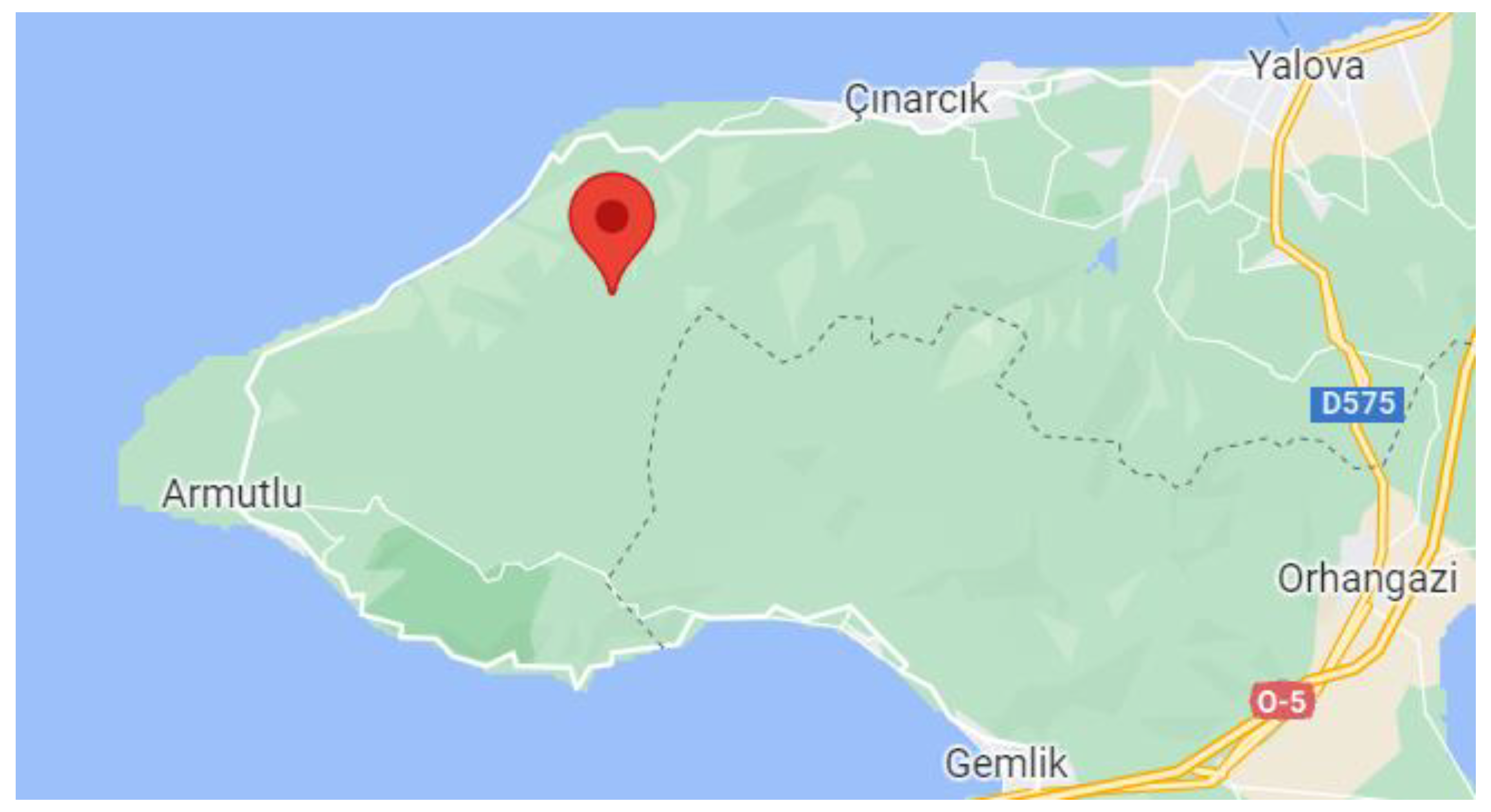
The internal data set contained information taken from the Esenkoy wind power plant shown in Figure 1 in the northwest part of Turkey (coordinate information “X: 40.58545 Y: 28.99035”), and this information was taken from a freely accessible wind turbine SCADA database [28]. The turbine used in the power plant was the N117/3600 model turbine produced by the Nordex company. Within the SCADA system, data such as wind speed (m/s), wind direction (°), theoretical power (kW), and active power (kW) belonging to the wind turbine for one year (1 January–31 December 2018) were periodically recorded.
The external data set, calculated using the latitude and longitude coordinates of the wind turbine, consisted of meteorological parameters provided by MERRA-2 Global (Modern Era Retrospective Analysis for Research and Applications) [29] and belonged to a specific date range (1 January–31 December 2018). In this data set, information regarding the turbine’s location is recorded hourly, including temperature (°C), precipitation amount (mm/hour), air density (kg/m3), solar radiation at ground level (W/m2), solar radiation above the atmosphere (W/m2), and cloud cover ratio. To achieve the most accurate results for predicting active power, merging two data sets within the same time interval was necessary. The first data set comprised 50,530 samples, among which 2030 missing data instances were identified. Therefore, the missing data were successfully imputed using the kNN algorithm, an ML technique employed for effectively completing missing data instances [31]. Subsequently, a new data set was created by filtering only the hourly data. Finally, the new data set was merged with the second data set, resulting in a final data set comprising 8760 observations.
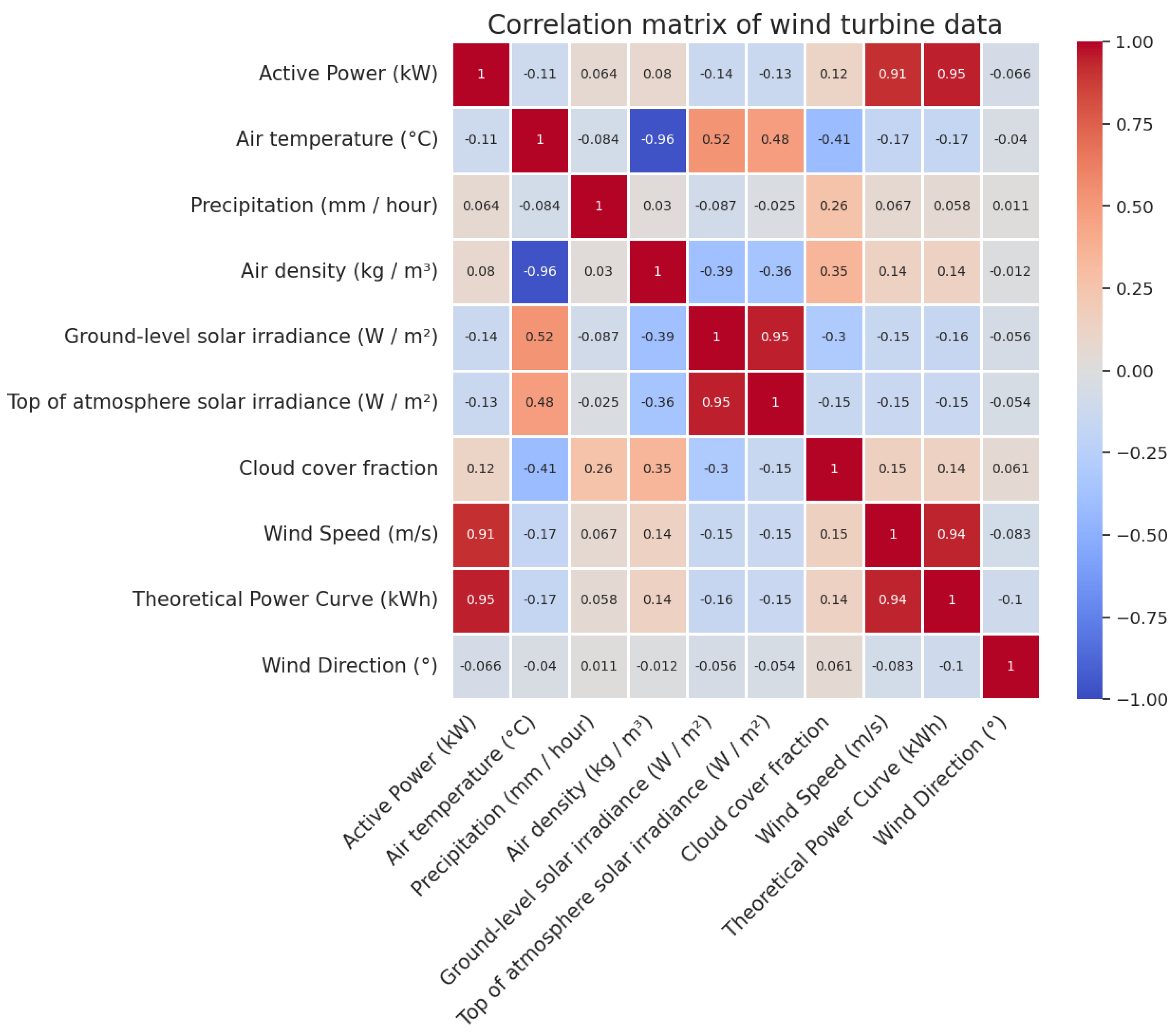
It is crucial to determine and quantify the strength of the impacts of the features in the data set on the generation of active wind power compared to other sources. Given the influence of multiple factors on power production, it is imperative to comprehend the interrelationships among these factors. To this end, a correlation matrix can be utilised to evaluate the correlations between the various elements. As illustrated in Figure 2, a visual depiction of the correlation coefficients between all input features and active power is provided. This graph expresses the correlation between one parameter and another numerically, ranging from −1 to +1. This correlation matrix shows how these independent input variables and the dependent output value affect each other. Upon analysing the correlation matrix presented in Figure 2, it becomes evident that the most significant influences on active power are attributed to the theoretical power curve and wind speed. Conversely, dynamic control negatively correlates with wind direction, temperature, and radiation rates. The temperature rise reduces air density, consequently negatively impacting wind power generation. Furthermore, heightened solar radiation elevates temperature levels, indirectly contributing to declining wind power potential. On the other hand, parameters such as air density, cloud cover ratio, and precipitation demonstrate a positive influence.
Some terms in the correlation matrix are here briefly explained. Rainfall has its quantity expressed in millimetres per hour. Air density pertains to the air per unit volume group, which indicates the air mass that fills a given space. Furthermore, solar radiation denotes the energy emitted by the sun through electromagnetic waves. Cloud cover ratio, also known as cloud cover percentage or cloudiness, pertains to the proportion of the sky obstructed by clouds at a particular location and time. Wind speed relates to the velocity at which air molecules move horizontally within the atmosphere. Wind direction denotes the direction from which the wind emanates.
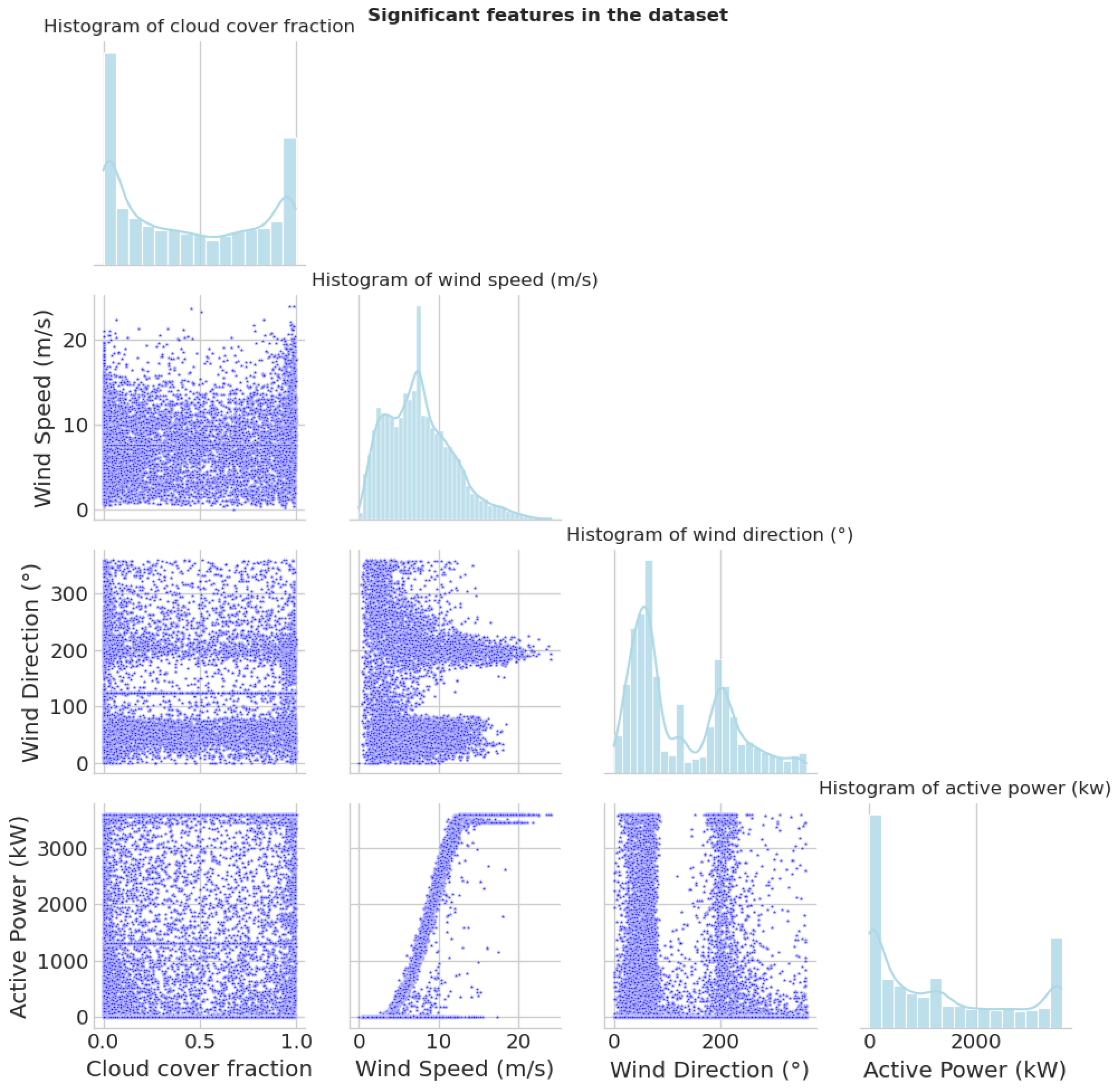
Figure 3 illustrates paired scatter plots that depict the interrelationships among various features. The scatter plots featuring a diagonal structure visually present histograms that outline the probability distribution of individual weather features. Scatter plots visualise the connections between these distinct features within the lower and upper triangles. Furthermore, each feature exemplifies its distribution alongside the other features. These paired scatter plots make alterations in one specific feature concerning all other features apparent.
Before model training, the removal of outliers is necessary. This process may involve handling missing data by either removing or imputing them, converting categorical variables into numerical values, and scaling the data. Wind speed values below 3.5 m/s or above 25.5 m/s need to be cleaned, as they do not align with the turbine’s appropriate power curve. This specific range represents values within which the turbine operates efficiently. Similarly, even if the wind speed exceeds 3.5 m/s, if the active power value is zero, this indicates that the turbine is not active during those time intervals. Lastly, data points with negative active power values should also be cleaned. I utilised the quartile method to clean outliers in the active power column, which involves identifying and removing outliers in a data set using the data’s quartiles (Q1 and Q3) along with the calculation of the interquartile range (IQR). Outliers were defined as values that fall outside the range of Q1 − 1.5 * IQR to Q3 + 1.5 * IQR, and these values were excluded from the data set. As a result of this process, 68 outliers were removed. kNN can be particularly effective in completing missing data, especially in the case of minor data gaps and when a suitable similarity measure is chosen. However, its performance may decrease with significant data gaps or high-dimensional data sets, so it is crucial to select an appropriate approach to address data incompleteness. In this study, the kNN technique was employed for imputing missing values, with the chosen value of K being 5. Figure 4 illustrates the wind power curve generated from the cleaned data after removing the outlier. This curve visually represents the variation of active and theoretical power for wind speed. Upon analysis of the chart, it is evident that the power production curve attains its utmost point when the wind speed approaches approximately 13 m/s and continues in a straight line.
The parameters used in active power prediction models have different vector values. Hence, normalising these input vectors provides several advantages to ensure their standardisation. Hence, the input features/tensors were scaled to a range of 0 to 1 before being fed into the DL layers using a min-max scaler. The normalised scale of a value was calculated using Equation (1):
Here, is the normalised value, is the original value, and max(x) and min(x) are the series’ most significant and minor values, respectively.
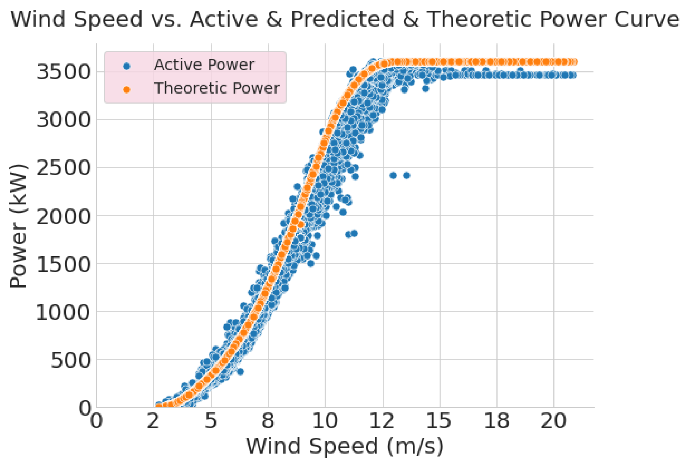
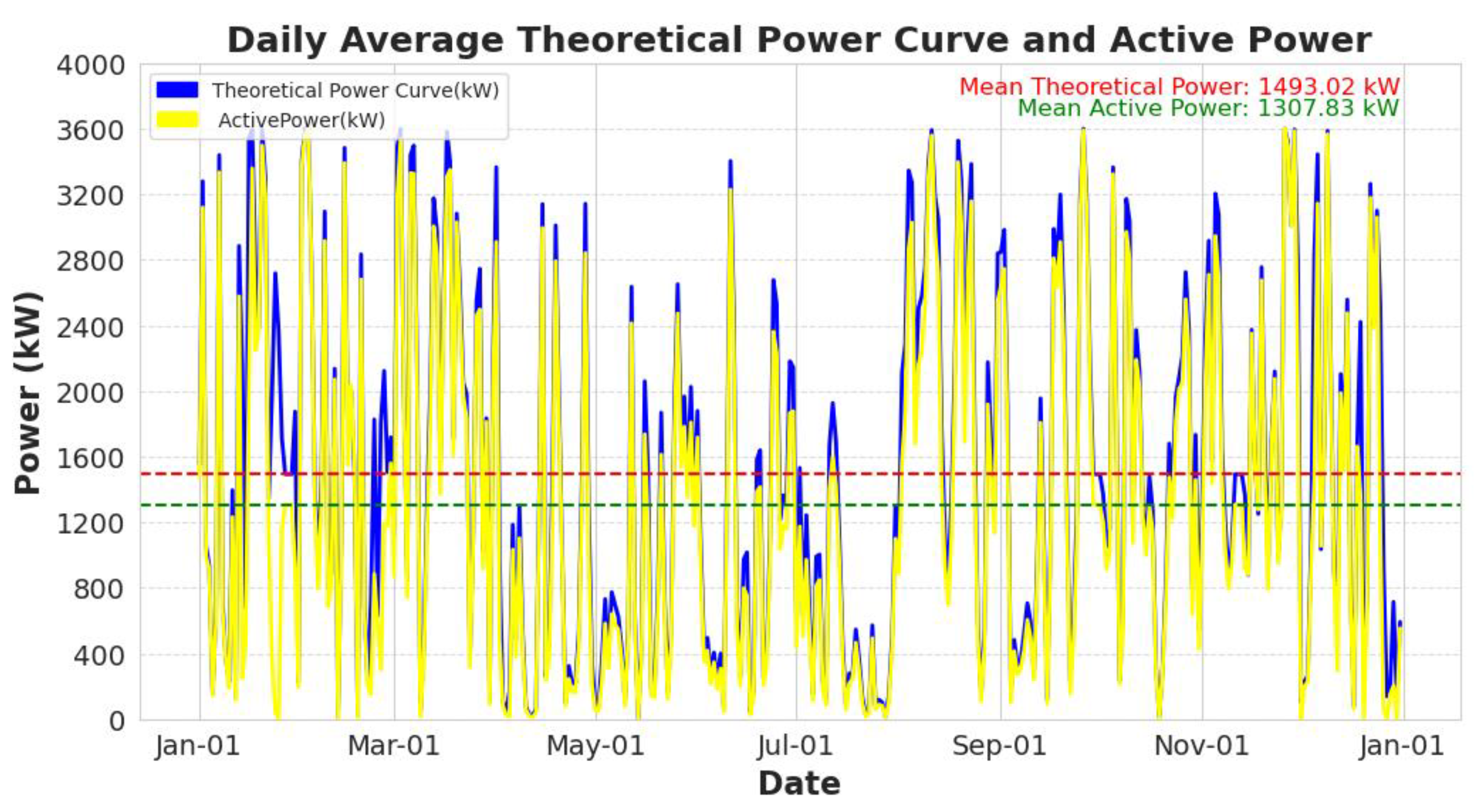
The designated power of the wind turbine indicated the maximum limit of the turbine’s power production, which was determined by the producer and authorised during the developmental stage. In Figure 5, theoretical and active power curves are presented visually. The theoretical power curve, otherwise referred to as the power–performance curve or simply the power curve, is a visual representation that elucidates the correlation between the wind speed and the power output of a wind turbine. Under ideal circumstances, it showcases the maximum quantity of power that a wind turbine can produce at varying wind speeds. Active power, frequently called absolute power, constitutes a fundamental concept in electrical engineering and power systems. It embodies the authentic power that a wind turbine generates in this study.
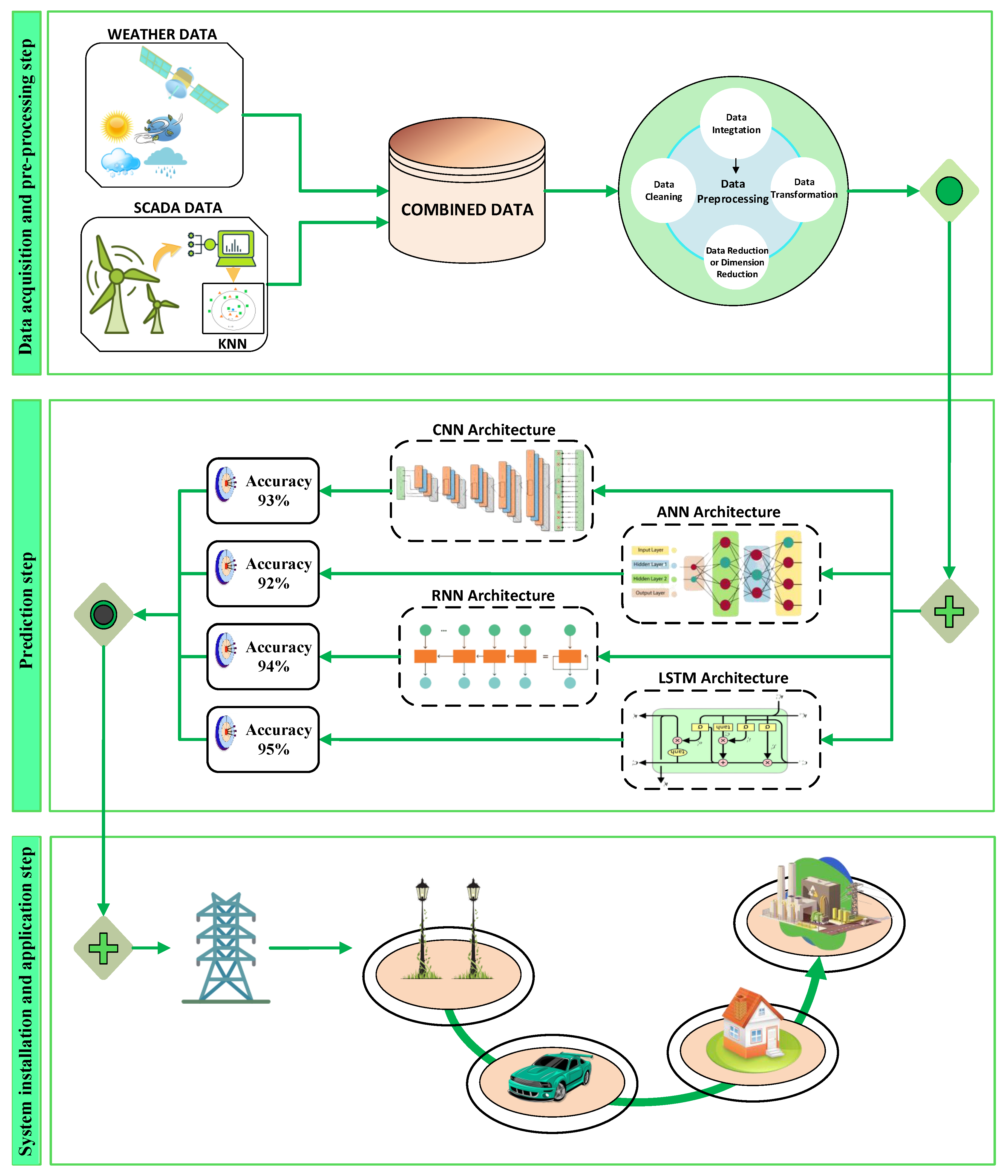
2.2. Proposed Model Architecture
The predictive performance of the intended models was evaluated using two data sets. The first data set pertains to internal wind turbine data, while the second comprises external weather-related data. These two data sets were merged to create a final data set with 8760 observations. The initial data set consisted of 50,530 samples, with 2030 missing data instances identified. The missing data was successfully imputed using the kNN algorithm to address this. Following this imputation, a new data set was generated by filtering only the hourly data points. After completing the data pre-processing steps, the data set was split into 75% for training and 25% for testing, using a random state value of 42. To maintain consistency among the data set’s features, the training and testing data were normalised using the min-max scaling method. During the training process, the parameter optimisation was carried out using the Adam (Adaptive Moment Estimation) algorithm, with an initial learning rate value set to 0.001. The MSE was employed as the loss function between the input and output. For each model, the number of epochs was developed to 100, and the batch size was 32. Subsequently, utilising these parameters, four different state-of-the-art and popular DL neural network architectures were compared to identify the optimal model for wind power estimation. Wind power was estimated using ANN, CNN, RNN, and LSTM methods using meteorological and turbine characteristic data.
Figure 6 represents a flowchart of the intended prediction model. In the study, the first model employs an ANN-based approach, the second model utilises a CNN-based DL architecture known for its success in large data sets, the third model incorporates an RNN architecture that is effective for time series data, and the fourth model employs an LSTM model, which yields successful results in analysing time series with more extended time intervals or complex structures. The objective is to identify the optimal hyperparameter combination that maximises model performance. To achieve this, a randomised search was employed, testing numerous hyperparameter settings to identify those that yielded the best performance.
Among ML methods, ANNs, RNNs, CNNs, and LSTMs are important in wind power forecasting. The ANN model is known for its ability to learn complex relationships and is useful for discovering patterns within large data sets. It also has a flexible structure and is effective for general predictions. CNNs are particularly successful in visual data processing but can also work well with time-series data. It is suitable for processing multidimensional data, such as wind speed and direction. RNNs are designed for processing time-series data and maintain information from previous time steps. This makes them a suitable choice for modelling changes over time. LSTMs are an improved version of RNNs and can handle long-term dependencies. They are well-suited for modelling various effects over time in wind power prediction.
2.2.1. Artificial Neural Network Structure
Artificial intelligence is dedicated to researching and developing methods that enable machines to exhibit human-like capabilities such as reasoning, judgment, emotional experience, language understanding, and problem-solving. One prominent approach in artificial intelligence is the ANN model, which is modelled after the structure of the human brain. However, the quantity of neurons within ANNs is established according to the demands of a given predicament, in contrast to the approximate 15 billion neurons within the human brain [32,33]. ANNs can learn from data and apply acquired knowledge, leading to their widespread utilisation in various domains, including but not limited to forecasting, classification, identification, and control. In this study, a feedforward neural network was constructed for wind power estimation, employing the general structure of a feedforward multilayer neural network, outlined as follows [34,35].
A multilayer feedforward network consists of various layers, including an input layer, an output layer, and one or more hidden layers positioned in between. The input layer is responsible for receiving the input data, which is then processed through the hidden layers, ultimately resulting in the generation of the final output by the output layer. The hidden layers play a fundamental role in effecting the transformation of the input data through a set of weighted connections and activation functions, thereby facilitating the network’s ability to comprehend intricate patterns and relationships within the data. Lastly, the output layer generates the final prediction based on the transformed information derived from the hidden layers. Table 1 shows that the ANN architecture begins with a dense layer in the first layer, consisting of 64 neurons and utilising the Rectified Linear Unit (ReLU) activation function. Following this, a second thick layer with 32 neurons and the ReLU activation function is employed. Finally, the model is completed with a dense layer with a single output and utilises the linear activation function.
2.2.2. Convolutional Neural Network Structure
Among various neural network architectures, CNNs are commonly employed for tasks such as image recognition, image classification, object detection, and facial recognition [36]. CNNs consist of neurons with trainable weights and biases, allowing them to capture and enhance low-level features in data. The convolutional layers in CNNs utilise filters to extract the spatial hierarchies of features, while the pooling layers reduce the spatial dimensionality of the extracted features. This hierarchical feature extraction process enables CNNs to effectively analyse and understand complex visual patterns in images. As a result, CNNs have achieved significant success in various computer vision tasks [37,38].
This method exhibits a practical capability for feature extraction. CNN structure parameters are given in Table 2. In the model, the data were first reshaped into a 1D array to make it suitable for the model and then presented as input. The model’s first layer was instantiated with 32 filters, a kernel size of 3, and the ReLU activation function. This layer was succeeded by a max-pooling layer that utilised a 2D pooling size. The third and final layer was the flattening layer, which flattened the data. The fourth layer comprised fully connected (dense) layers, where neurons combined their inputs. The first thick layer had 64 neurons with the ReLU activation function, while the second dense layer had 32 neurons with the ReLU activation function. The final layer, composed of a solitary output neuron, was represented by the output layer and employed the linear activation function.
2.2.3. Recurrent Neural Networks Structure
RNNs have been utilised to assimilate the short-term temporal dependency on wind power. RNNs can consider antecedent information and formulate a prediction [39]. RNNs learn their predictions by adjusting ML parameters through backpropagation and gradient descent. RNNs are designed to process input data and model dependencies in sequential data. As a result, RNNs typically consist of multiple neuron layers, with each layer improving by utilising the previous layer’s outputs.
RNN structure parameters are shown in Table 3. The proposed architecture comprised 32 neurons with a ReLU activation function in the first layer. Following this, a flattened layer was implemented, after which, a dense layer comprising 64 neurons and utilising a ReLU activation function was employed. This was then succeeded by another thick layer containing 32 neurons and a ReLU activation function. Finally, the model was completed with a dense layer with a single output and a linear activation function.
2.2.4. Long Short-Term Memory Structure
LSTMs are a variant of RNNs that can capture relationships in time series or sequential data by storing information from previous steps in their memory. By incorporating specialised memory cells, LSTMs can retain relevant information over longer sequences and selectively update or forget information as needed [16]. The memory mechanism employed by LSTMs facilitates their ability to surmount the obstacles presented by the vanishing or exploding gradients that afflict conventional RNNs. Therefore, this mechanism augments the proficiency of LSTMs in efficiently grasping and exploiting enduring correlations inherent in a given data set [40].
LSTM structure parameters are shown in Table 4. The architecture of our model started with a Conv1D layer, which consisted of 32 filters, a kernel size of 3, and a ReLU activation function. This layer was initially employed to effectively capture local patterns and enable the extraction of relational meanings from the intended sequences before the LSTM layer. Subsequently, an LSTM layer with 64 neurons and a ReLU activation function was employed. The third layer continued with a dense layer of 64 neurons and a ReLU activation function. Incorporating a ReLU activation function, 32 neurons were utilised in the fourth layer. Due to its singular output, a linear activation function was employed in the last layer to finalise the model architecture.
2.3. Error Metrics
This paper employed various statistical methods to evaluate the accuracy of the ANN-RNN-CNN-LSTM model’s predictions. These criteria encompassed commonly utilised error metrics, including RMSE, MAE, and MSE. These were employed to assess the disparity between the predicted and actual values, disregarding the direction of errors or their compensatory effects. Error metrics quantitatively measure how close predictions are to actual data. This helps us evaluate how accurate predictions are. Accurate predictions are crucial for reliable applications like energy resources.
MAE represents the measurement of the absolute difference between the predicted and actual variables. RMSE represents the standard deviation in prediction errors, with a lower value indicative of a superior model. If the RMSE values of training and testing samples fall within a limited range, the model is considered satisfactory without overfitting. MSE represents the average of the square of errors. The aim was to achieve low MAE, MAPE, and RMSE values indicative of enhanced predictive accuracy. Statistical indicators like MSE, RMSE, and MAE have their advantages and disadvantages. MSE assigns greater weight to larger errors, which makes it more sensitive to outliers or significant errors. This property can be advantageous when dealing with large errors that are particularly costly or need to be minimised. MSE has excellent mathematical properties. It is differentiable, making it suitable for optimisation algorithms and the basis for many statistical methods. While its sensitivity to errors can be advantageous, it can also be a disadvantage. Outliers can disproportionately impact MSE, potentially leading to an inaccurate assessment of model performance. MAE is less sensitive to outliers compared to MSE. It gives equal weight to all errors, which can provide a more robust performance measure in the presence of outliers. MAE gives equal weight to all errors; it may not penalise large errors as heavily as MSE. This can be a disadvantage when large errors need to be minimised or when they are particularly costly [41,42,43].
R2 functions as a statistical metric that denotes the degree to which the alteration in the independent variable accounts for the variance observed in the dependent variable. It is noteworthy that the R2 value lay between 1 and 0. A higher R2 value signifies a better fit of the regression line, indicating that changes in the dependent variable are primarily attributed to changes in the independent variable. Equations (2)–(5) provide the formulas for R2, RMSE, MSE, and MAE [44,45].
Here represent the predicted value, actual value, sample size, mean predicted value, and mean actual value, respectively.
3. Results and Discussion
This section examines the performance results obtained based on the ML models developed in previous areas. All models were tested and explained in a Jupiter Notebook development environment running Python 3.9.5. The machine had hardware specifications, including a dual-core Intel(R) Xeon(R) CPU at 2.20 GHz processor, 32 GB 3200 MHz DDR3 RAM, and a 16 GB Nvidia Tesla P100 GPU. The TensorFlow 2.x library was used to build DL architectures. TensorFlow is a library that facilitates the efficient processing of large data sets, especially the flow of multidimensional arrays or tensors from one layer to another in neural networks.
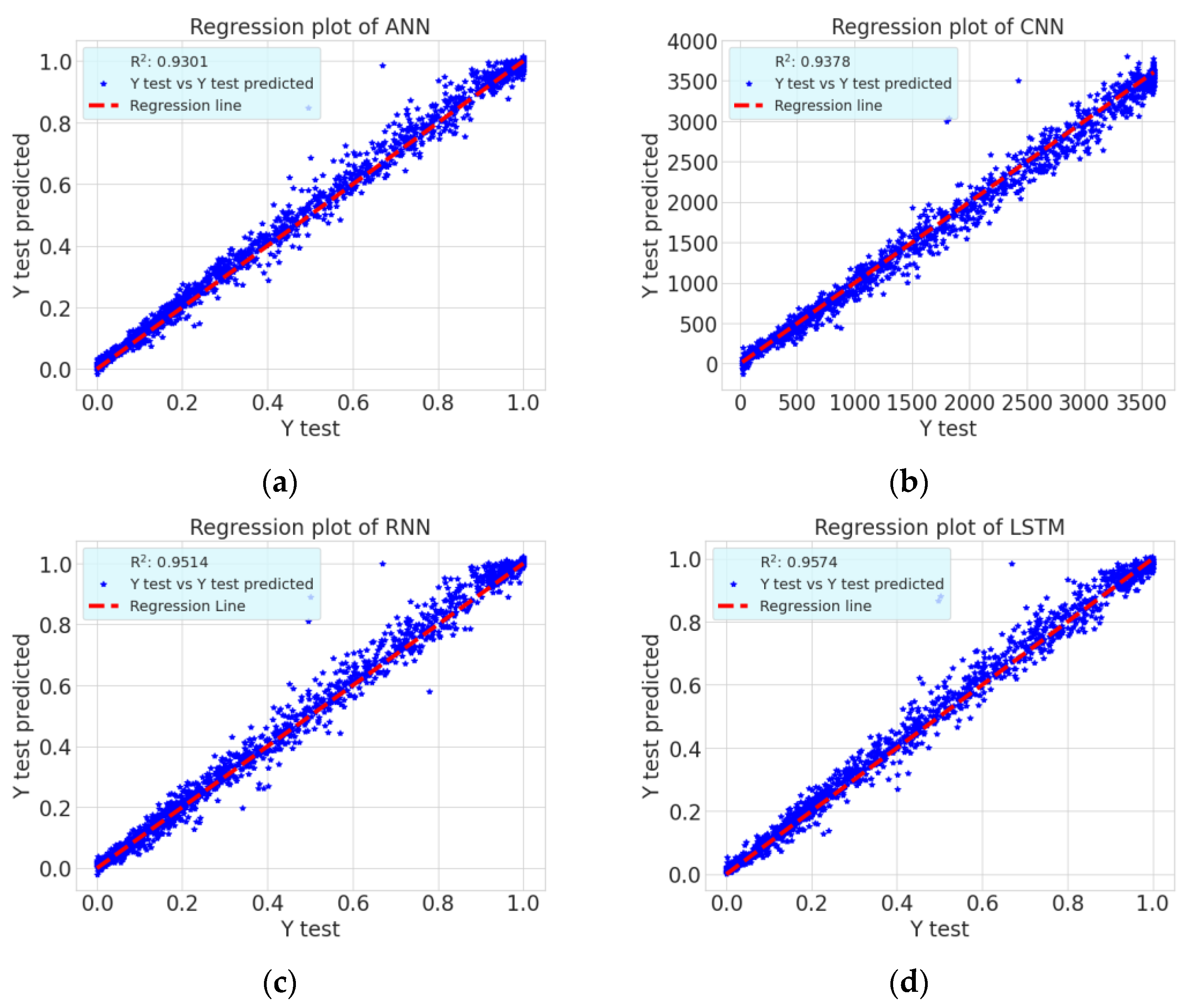
The model trained competently with the ANN, CNN, RNN, and LSTM methods, demonstrating their ability to accurately predict the test data set, as shown in Figure 7. Figure 7 shows linear regression plots for the methods. A linear regression plot is a graph that visually represents the relationship between two variables. Upon examining the graphs, it was observed that the LSTM method exhibited the best prediction performance, with an R2 value of 0.9574.
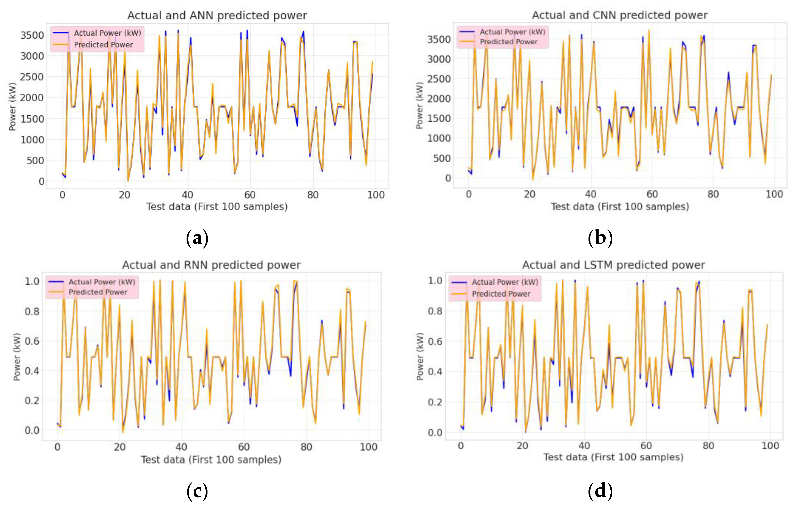
By comparing the initial 100 samples of the test data and the first 100 samples predicted by the ANN, CNN, RNN, and LSTM models, it was established that there exists a concordant relationship between the model’s predictions and the test data. This correlation is demonstrated in Figure 8.
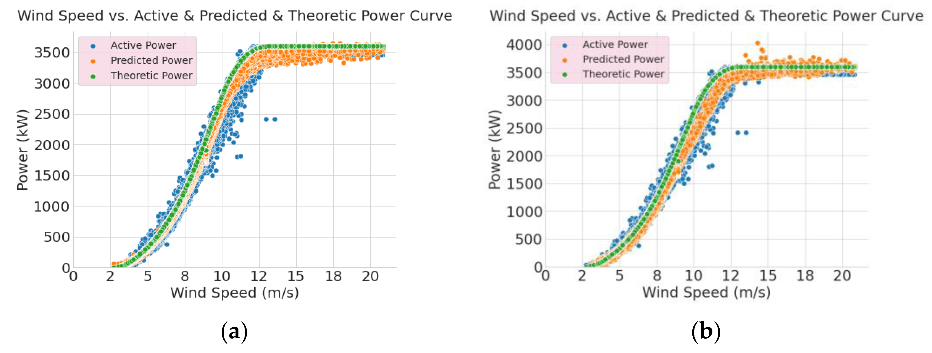
Figure 9 depicts a scatterplot illustrating the correlation between wind speed (m/s) and the turbine’s active power generation (kW). The plot also includes the estimated functional power value and the theoretical power curve. Upon closer examination of the graph, it becomes evident that the four models’ predicted active power values exceeded the turbine’s maximum power output, particularly when wind speeds exceeded approximately 13 m/s. The main reason for the higher prediction accuracy provided by CNNs compared to ANNs was due to the feature extraction capabilities of CNNs. Notably, under low wind speed conditions, CNNs exhibited a high level of performance in generating more accurate results. In contrast, the prediction values showed lower accuracy under challenging conditions like high wind speeds.
Consequently, during low wind speeds, CNNs effectively leveraged their advanced feature extraction prowess to discern pivotal data patterns, thereby enhancing the precision of predictions. However, within intricate contexts like high wind speeds, the projections sometimes carried a decreased level of accuracy. These findings underscore CNNs as proficient instruments for addressing problems contingent on temporal fluctuations, as seen in wind power prediction. Nonetheless, it is discernible that the extent of this efficacy can fluctuate based on the wind speed magnitude in specific cases. This situation provides a significant perspective on how CNNs’ feature extraction capabilities prove impactful in applications like wind power prediction.
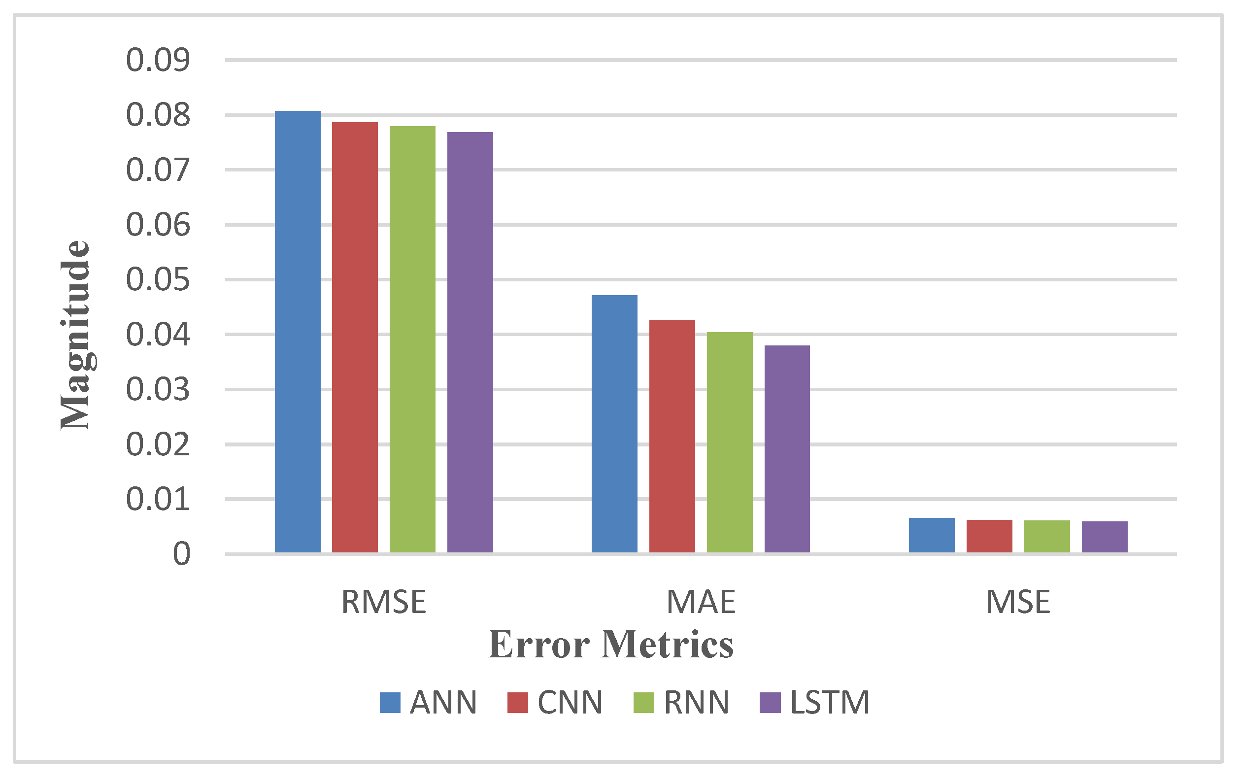
Figure 10 graphically shows the comparison of MSE, RMSE, and MAE error metrics for the four methods. When the graphs are examined, it is observed that the lowest error metrics belong to LSTM.
Table 5 presents the R2, MSE, RMSE, and MAE outcomes for the testing and training data sets that predicted wind power.
As a result, since the RNN architecture could heal itself with the outputs from the previous layer, it performed more successfully than ANNs and CNNs, especially in sequential data sets. This finding indicates that upon examination of the graphs, the estimated values tended to be closer to the actual values. LSTM is an RNN model utilised in sequential or time series analysis. Particularly in sequential data sets, it demonstrates superior performance due to the self-healing capability of LSTMs. As a result, it achieves higher prediction success compared to other models.
In contrast to Tuerxun et al.’s study [20], which employed 3200 data points, this study utilised 8760 data points. They have proposed various prediction models. R2 metric was used to compare these models. They employed a hybrid approach by combining three methods, achieving the highest R2 value of 0.98. However, they obtained lower R2 values with three other hybrid methods, specifically 0.48, 0.82, and 0.80. Their study involved sequential variation mode decomposition (SVMD) to parse pre-processed wind speed data, then optimised the LSTM algorithm through PSO, TSO, and MTSO optimisation techniques. This implies that their approach involved a more complex model and additional data processing stages.
In contrast, our study proposed a simpler model and achieved a high R2 score of 0.95. Furthermore, we incorporated real climatic conditions and turbine regime periods from 2018, making our method more suitable for real-world applications. This demonstrates that our work has a broader range of applications, and the results we obtained can be readily applied in real-world conditions.
4. Conclusions
Due to the inherent variability of wind power, forecasting presents a formidable challenge. Furthermore, successfully integrating wind power into primary power grids is a significant obstacle. As such, in this study, popular ML methods (ANN, RNN, CNN, and LSTM algorithms) with high predictive performance are examined to predict wind power. The algorithms’ performances were assessed using statistical metrics, namely, MAE, RMSE, MSE, and R2. Algorithms characterised by minimal errors indicated the most desirable and precise methodology. When the results presented above are examined, it can be understood that the proposed ML methods enable successful wind power estimation.
To train and evaluate ML models, a SCADA system was employed to gather empirical data from January to December 2018, with a sampling frequency of 10 min. Additionally, the MERRA-2 Global data set, made available by NASA, was employed to evaluate the impact of meteorological data on wind power. When the correlation matrix between input parameters and active management is examined, it is observed that the strongest correlation among weather parameters is a correlation of 0.12 between cloud cover fraction and dynamic power. When analysing the correlation matrix, it becomes apparent that a notably robust correlation (0.95) exists between active power and the theoretical power curve. Then, it is observed that there is a correlation (0.91) between operational management and wind speed.
The results showed that the LSTM, RNN, CNN, and ANN algorithms are powerful in forecasting wind power. Among these algorithms, LSTM is the best algorithm, with an R2 value of 0.9574, MAE of 0.0209, MSE of 0.0038, and RMSE of 0.0614. DL models possess the ability to acquire intricate connections within data sets. The LSTM model utilised in this study stands out among deep learning models due to its capability to manage long-term dependencies effectively. As a result, LSTMs emerge as a valuable instrument for resolving issues involving time-dependent data, as exemplified by their application in wind power prediction. In applications like wind power forecasting, temporal changes over time are crucial. LSTMs can model complex relationships over time by preserving information from previous time steps, which enables them to be more accurate in predicting future wind power. This highlights LSTMs’ valuable role in addressing challenges related to time-dependent data, as evidenced by their successful application in wind power prediction. Wind power forecasting is critical for energy production planning. The accurate predictions provided by LSTMs and similar deep learning models can enhance the efficiency of wind energy production scheduling. Based on these forecasts, energy companies can optimise their resource allocation and grid management. Accurate wind power predictions contribute to grid stability and reliability. Power grid operators can use these forecasts to balance energy supply and demand better, reducing the risk of blackouts and ensuring uninterrupted energy supply to consumers. Improved wind power prediction can lead to the better integration of renewable energy sources into the grid. This, in turn, reduces reliance on fossil fuels, decreases greenhouse gas emissions, and contributes to a more sustainable and environmentally friendly energy ecosystem. The limitations of this study are as follows: it should be noted that only limited data from the year 2018 were used. Having more data typically enhances the ability to make better predictions. A larger data set allows for greater model complexity and depth. Models can make more general and reliable predictions if more data are available. Constraints on the amount of data can impact the sharpness and accuracy of predictions. Deep learning models often require a large amount of data. Limited data can negatively impact the performance of these models and increase the risk of overfitting. Deep learning models typically require significant computational resources. Particularly, high-performance computers or GPUs may be needed to train large models. While models like RNN and LSTM are designed to handle time series data, capturing long-term dependencies can sometimes be challenging. Future work will evaluate the accuracy of prediction models by incorporating hybrid and ML approaches. Many studies in the literature show that hybrid models give more successful results. More accurate and general results will be presented by comparing the prediction performances of hybrid models and normal machine learning models.
Funding
This research received no external funding.
Institutional Review Board Statement
Not applicable.
Informed Consent Statement
Not applicable.
Data Availability Statement
The data presented in this study are openly available in [Kaggle] at [https://www.kaggle.com/datasets/berkerisen/wind-turbine-scada-dataset] and [renewables.ninja] at [https://www.renewables.ninja] (accessed on 15 June 2023).
Conflicts of Interest
The author declares that they have no known competing financial interest or personal relationships that could have appeared to influence the work reported in this paper.
References
- Li, H. Short-term wind power prediction via spatial-temporal analysis and deep residual networks. Front. Energy Res. 2022, 10, 662. [Google Scholar] [CrossRef]
- Yetis, Y.; Tehrani, K.; Jamshidi, M. Wind Speed Forecasting using Machine Learning Approach based on Meteorological Data case study. Energy Environ. Res. 2022, 12, 2. [Google Scholar] [CrossRef]
- Zhang, H.; Yue, D.; Dou, C.; Li, K.; Hancke, G. Two-Step Wind Power Prediction Approach with Improved Complementary Ensemble Empirical Mode Decomposition and Reinforcement Learning. IEEE Syst. J. 2022, 16, 2545. [Google Scholar] [CrossRef]
- Ummels, B.; Gibescu, M.; Pelgrum, E.; Kling, W.; Brand, A. Impacts of Wind Power on Thermal Generation Unit Commitment and Dispatch. IEEE Trans. Energy Convers. 2007, 22, 44–51. [Google Scholar] [CrossRef]
- Damchi, Y.; Eivazi, A. Power Swing and Fault Detection in the Presence of Wind Farms Using Generator Speed Zero-Crossing Moment. Int. Trans. Electr. Energy Syst. 2022, 2022, 2569810. [Google Scholar] [CrossRef]
- Rahman, M.M.; Shakeri, M.; Tiong, S.K.; Khatun, F.; Amin, N.; Pasupuleti, J.; Hasan, M.K. Prospective Methodologies in Hybrid Renewable Energy Systems for Energy Prediction Using Artificial Neural Networks. Sustainability 2021, 13, 2393. [Google Scholar] [CrossRef]
- Ray, B.; Shah, R.; Islam, M.; Islam, S. A New Data-Driven Long-Term Solar Yield Analysis Model of Photovoltaic Power Plants. IEEE Access 2020, 8, 136223. [Google Scholar] [CrossRef]
- Abdalla, A.; Nazir, M.; Jiang, M.; Kadhem, A.; Wahab, N.; Cao, S.; Ji, R. Metaheuristic searching genetic algorithm based reliability assessment of hybrid power generation system. Energy Explor. Exploit. 2020, 39, 1. [Google Scholar] [CrossRef]
- Lahouar, A.; Ben Hadj Slama, J. Hour-ahead wind power forecast based on random forests. Renew. Energy 2017, 109, 529–541. [Google Scholar] [CrossRef]
- Sarp, A.; Mengüç, E.; Peker, M.; Güvenç, B. Data-Adaptive Censoring for Short-Term Wind Speed Predictors Based on MLP, RNN, and SVM. IEEE Syst. J. 2022, 16, 3625. [Google Scholar] [CrossRef]
- Li, J.; Mao, J. Ultra-short-term wind power prediction using BP neural network. In Proceedings of the 2014 9th IEEE Conference on Industrial Electronics and Applications, Hangzhou, China, 9–11 June 2014; pp. 2001–2006. [Google Scholar] [CrossRef]
- Ma, J.; Ma, X. A review of forecasting algorithms and energy management strategies for microgrids. Syst. Sci. Control Eng. 2018, 6, 237–248. [Google Scholar] [CrossRef]
- Chu, X.; Bai, W.; Sun, Y.; Li, W.; Liu, C.; Song, H. A Machine Learning-Based Method for Wind Fields Forecasting Utilizing GNSS Radio Occultation Data. IEEE Access 2022, 10, 30258. [Google Scholar] [CrossRef]
- Meng, Y.; Chang, C.; Huo, J.; Zhang, Y.; Al-Neshmi, H.; Xu, J.; Xie, T. Research on Ultra-Short-Term Prediction Model of Wind Power Based on Attention Mechanism and CNN. BiGRU Combined. Front. Energy Res. 2022, 10, 1. [Google Scholar] [CrossRef]
- Cheng, W.; Feng, J.; Wang, Y.; Peng, Z.; Cheng, H.; Ren, X.; Shuai, Y.; Zang, S.; Liu, H.; Pu, X.; et al. High precision reconstruction of silicon photonics chaos with stacked CNN-LSTM neural networks. Chaos 2022, 32, 053112. [Google Scholar] [CrossRef]
- Solas, M.; Cepeda, N.; Viegas, J.L. Convolutional Neural Network for Short-Term Wind Power Forecasting. In Proceedings of the 2019 IEEE PES Innovative Smart Grid Technologies Europe (ISGT-Europe), Bucharest, Romania, 29 September–2 October 2019; Institute of Electrical and Electronics Engineers: Piscataway, NJ, USA, 2019; pp. 1–5. [Google Scholar] [CrossRef]
- Liu, T.; Huang, Z.; Tian, L.; Zhu, Y.; Wang, H.; Feng, S. Enhancing Wind Turbine Power Forecast via Convolutional Neural Network. Electronics 2021, 10, 261. [Google Scholar] [CrossRef]
- Agarwal, K.; Vadhera, S. Short-term Wind Speed Prediction using ANN. In Proceedings of the 2022 International Conference on Sustainable Computing and Data Communication Systems (ICSCDS), Erode, India, 7–9 April 2022. [Google Scholar] [CrossRef]
- Chimaobi, A.; Ye, L. Using Convolutional Neural Network for Image Classification and Segmentation. Comput. Eng. Intell. Syst. 2022, 13, 21. [Google Scholar] [CrossRef]
- Tuerxun, W.; Xu, C.; Guo, H.; Guo, L.; Zeng, N.; Cheng, Z. An ultra-short-term wind speed prediction model using LSTM based on modified tuna swarm optimisation and successive variational mode decomposition. Energy Sci. Eng. 2022, 10, 3001. [Google Scholar] [CrossRef]
- Hao, Y.; Tian, C. A novel two-stage forecasting model based on error factor and ensemble method for multi-step wind power forecasting. Appl. Energy 2019, 238, 368–383. [Google Scholar] [CrossRef]
- Sun, Y.; Li, Z.; Yu, X.; Li, B.; Yang, M. Research on Ultra-Short-Term Wind Power Prediction Considering Source Relevance. IEEE Access 2020, 8, 147703–147710. [Google Scholar] [CrossRef]
- Haq, K.; Harigovindan, V. Water Quality Prediction for Smart Aquaculture Using Hybrid Deep Learning Models. IEEE Access 2022, 10, 60078. [Google Scholar] [CrossRef]
- Liu, X.; Li, X.; Tian, J.; Wang, Y.; Xiao, G.; Wang, P. Day-Ahead Economic Dispatch of Renewable Energy System Considering Wind and Photovoltaic Predicted Output. Int. Trans. Electr. Energy Syst. 2022, 2022, 14. [Google Scholar] [CrossRef]
- Ren, J.; Yu, Z.; Gao, G.; Yu, G.; Yu, J. A CNN-LSTM-LightGBM-based short-term wind power prediction method based on attention mechanism. Energy Rep. 2022, 8, 437–443. [Google Scholar] [CrossRef]
- Liu, J.; Shi, Q.; Han, R.; Yang, J. A Hybrid GA–PSO–CNN Model for Ultra-Short-Term Wind Power Forecasting. Energies 2021, 14, 6500. [Google Scholar] [CrossRef]
- Çelebi, S.B.; Emiroğlu, B.G. Leveraging Deep Learning for Enhanced Detection of Alzheimer’s Disease Through Morphometric Analysis of Brain Images. Trait. Du Signal 2023, 40, 1355–1365. [Google Scholar] [CrossRef]
- Available online: https://www.kaggle.com/datasets/berkerisen/wind-turbine-scada-dataset (accessed on 15 June 2023).
- Available online: https://www.renewables.ninja (accessed on 15 June 2023).
- Available online: https://www.google.com/maps (accessed on 15 June 2023).
- Triguero, I.; García-Gil, D.; Maillo, J.; Luengo, J.; García, S.; Herrera, F. Transforming big data into smart data: An insight on the use of the k-nearest neighbors algorithm to obtain quality data. Wiley Interdiscip. Rev. Data Min. Knowl. Discov. 2019, 9, e1289. [Google Scholar] [CrossRef]
- Jiang, D.; Zhang, H.; Kumar, H.; Naveed, Q.; Takhi, C.; Jagota, V.; Jain, R. Automatic Control Model of Power Information System Access Based on Artificial Intelligence Technology. Math. Probl. Eng. 2022, 2022, 5677634. [Google Scholar] [CrossRef]
- Birecikli, B.; Karaman, Ö.A.; Çelebi, S.B.; Turgut, A. Failure load prediction of adhesively bonded GFRP composite joints using artificial neural networks. J. Mech. Sci. Technol. 2020, 34, 4631–4640. [Google Scholar] [CrossRef]
- Mostafa, K.; Zisis, I.; Moustafa, M.A. Machine Learning Techniques in Structural Wind Engineering: A State-of-the-Art Review. Appl. Sci. 2022, 12, 5232. [Google Scholar] [CrossRef]
- Babbar, S.; Langah, T. Wind Power Prediction Using Neural Networks with Different Training Models. Indones. J. Innov. Appl. Sci. (IJIAS) 2022, 2, 12–17. [Google Scholar] [CrossRef]
- Çalışkan, A. Diagnosis of malaria disease by integrating chi-square feature selection algorithm with convolutional neural networks and autoencoder network. Trans. Inst. Meas. Control 2023, 45, 975–985. [Google Scholar] [CrossRef]
- Acero-Cuellar, T.; Bianco, F.; Dobler, G.; Sako, M.; Qu, H. There’s no difference: Convolutional Neural Networks for transient detection without template subtraction. arXiv 2022, arXiv:2203.07390. [Google Scholar] [CrossRef]
- Çelebi, S.B.; Emiroğlu, B.G. A Novel Deep Dense Block-Based Model for Detecting Alzheimer’s Disease. Appl. Sci. 2023, 13, 8686. [Google Scholar] [CrossRef]
- Salah, S.; Alsamamra, H.R.; Shoqeir, J.H. Exploring Wind Speed for Energy Considerations in Eastern Jerusalem-Palestine Using Machine-Learning Algorithms. Energies 2022, 15, 2602. [Google Scholar] [CrossRef]
- Muneer, A.; Ali, R.; Almaghthawi, A.; Taib, S.; Alghamdi, A.; Ghaleb, E. Short-term residential load forecasting using long short-term memory recurrent neural network. Int. J. Electr. Comput. Eng. (IJECE) 2022, 12, 5589. [Google Scholar] [CrossRef]
- Wang, C.-C.; Chang, H.-T.; Chien, C.-H. Hybrid LSTM-ARMA Demand-Forecasting Model Based on Error Compensation for Integrated Circuit Tray Manufacturing. Mathematics 2022, 10, 2158. [Google Scholar] [CrossRef]
- Saglam, M.; Spataru, C.; Karaman, O.A. Electricity Demand Forecasting with Use of Artificial Intelligence: The Case of Gokceada Island. Energies 2022, 15, 5950. [Google Scholar] [CrossRef]
- Saglam, M.; Spataru, C.; Karaman, O.A. Forecasting Electricity Demand in Turkey Using Optimisation and Machine Learning Algorithms. Energies 2023, 16, 4499. [Google Scholar] [CrossRef]
- Karaman, Ö.A. Performance evaluation of seasonal solar irradiation models—Case study: Karapınar town, Turkey. Case Stud. Therm. Eng. 2023, 49, 103228. [Google Scholar] [CrossRef]
- Karaman, Ö.A.; Ağır, T.T.; Arsel, İ. Estimation of solar radiation using modern methods. Alex. Eng. J. 2021, 60, 2447–2455. [Google Scholar] [CrossRef]
Figure 1.
Esenkoy wind turbine location [30].
Figure 1.
Esenkoy wind turbine location [30].

Figure 2.
Correlation of input parameters with active power.

Figure 3.
Histograms and intensities for variables.

Figure 4.
Wind speed vs. power curve with the raw data set.

Figure 5.
Theoretical power curve and active power.

Figure 6.
Flowchart of prediction model.

Figure 7.
Regression plot of test data and predicted values by (a) ANN, (b) CNN, (c) RNN, and (d) LSTM models.
Figure 7.
Regression plot of test data and predicted values by (a) ANN, (b) CNN, (c) RNN, and (d) LSTM models.

Figure 8.
Comparison of test data with predicted test data by (a) ANN, (b) CNN, (c) RNN, and (d) LSTM methods.
Figure 8.
Comparison of test data with predicted test data by (a) ANN, (b) CNN, (c) RNN, and (d) LSTM methods.

Figure 9.
Active power, estimated active power, and theoretical power curve by (a) ANN, (b) CNN, (c) RNN, and (d) LSTM methods.
Figure 9.
Active power, estimated active power, and theoretical power curve by (a) ANN, (b) CNN, (c) RNN, and (d) LSTM methods.


Figure 10.
Error metric comparison of methods.


Table 1.
ANN structure parameters.
| Layer | Output Shape | Parameter |
|---|---|---|
| Dense | (, 64) | 704 |
| Dense | (, 32) | 2080 |
| Dense | (, 1) | 33 |
| Total Parameter | 2817 |
Table 2.
CNN structure parameters.
| Layer | Output Shape | Parameter |
|---|---|---|
| Conv1D | (, 8, 32) | 128 |
| Max Pooling 1D | (, 4, 32) | 0 |
| Flatten | (, 128) | 0 |
| Dense | (, 64) | 8256 |
| Dense | (, 32) | 2080 |
| Dense | (, 1) | 33 |
| Total Parameter | 10,497 |
Table 3.
RNN structure parameters.
| Layer | Output Shape | Parameter |
|---|---|---|
| Simple RNN | (, 32) | 1088 |
| Flatten | (, 32) | 0 |
| Dense | (, 64) | 2112 |
| Dense | (, 32) | 2080 |
| Dense | (, 1) | 33 |
| Total Parameter | 5313 |
Table 4.
LSTM structure parameters.
| Layer | Output Shape | Parameter |
|---|---|---|
| Conv1D | (, 8, 32) | 128 |
| LSTM | (, 64) | 24,832 |
| Dense | (, 64) | 4160 |
| Dense | (, 32) | 2080 |
| Dense | (, 1) | 33 |
| Total Parameter | 31,233 |
Table 5.
Performance metrics of models.
| Machine Learning Models | Performance Evaluation on Training Data Set | Performance Evaluation on Testing Data Set | Training Time (s) | ||||||
|---|---|---|---|---|---|---|---|---|---|
| MAE | MSE | RMSE | R2 | MAE | MSE | RMSE | R2 | ||
| ANN | 0.0224 | 0.0057 | 0.0757 | 0.9345 | 0.0245 | 0.0062 | 0.0787 | 0.9301 | 81.6 |
| CNN | 0.0218 | 0.0054 | 0.0732 | 0.9388 | 0.0235 | 0.0055 | 0.0742 | 0.9378 | 85.3 |
| RNN | 0.0196 | 0.0038 | 0.0615 | 0.9567 | 0.0218 | 0.0043 | 0.0656 | 0.9514 | 82.7 |
| LSTM | 0.0179 | 0.0027 | 0.0517 | 0.9694 | 0.0209 | 0.0038 | 0.0614 | 0.9574 | 85.8 |
Disclaimer/Publisher’s Note: The statements, opinions and data contained in all publications are solely those of the individual author(s) and contributor(s) and not of MDPI and/or the editor(s). MDPI and/or the editor(s) disclaim responsibility for any injury to people or property resulting from any ideas, methods, instructions or products referred to in the content. |
© 2023 by the author. Licensee MDPI, Basel, Switzerland. This article is an open access article distributed under the terms and conditions of the Creative Commons Attribution (CC BY) license (https://creativecommons.org/licenses/by/4.0/).
Share and Cite
MDPI and ACS Style
Karaman, Ö.A. Prediction of Wind Power with Machine Learning Models. Appl. Sci. 2023, 13, 11455. https://doi.org/10.3390/app132011455
AMA Style
Karaman ÖA. Prediction of Wind Power with Machine Learning Models. Applied Sciences. 2023; 13(20):11455. https://doi.org/10.3390/app132011455
Chicago/Turabian StyleKaraman, Ömer Ali. 2023. "Prediction of Wind Power with Machine Learning Models" Applied Sciences 13, no. 20: 11455. https://doi.org/10.3390/app132011455
Note that from the first issue of 2016, this journal uses article numbers instead of page numbers. See further details here.