Lane Line Type Recognition Based on Improved YOLOv5

Abstract

The recognition of lane line type plays an important role in the perception of advanced driver assistance systems (ADAS). In actual vehicle driving on roads, there are a variety of lane line type and complex road conditions which present significant challenges to ADAS. To address this problem, this paper proposes an improved YOLOv5 method for recognising lane line type. This method can accurately and quickly identify the types of lane lines and can show good recognition results in harsh environments. The main strategy of this method includes the following steps: first, the FasterNet lightweight network is introduced into all the concentrated-comprehensive convolution (C3) modules in the network to accelerate the inference speed and reduce the number of parameters. Then, the efficient channel attention (ECA) mechanism is integrated into the backbone network to extract image feature information and improve the model’s detection accuracy. Finally, the sigmoid intersection over union (SIoU) loss function is used to replace the original generalised intersection over union (GIoU) loss function to further enhance the robustness of the model. Through experiments, the improved YOLOv5s algorithm achieves 95.1% of mAP@0.5 and 95.2 frame·s⁻¹ of FPS, which can satisfy the demand of ADAS for accuracy and real-time performance. And the number of model parameters are only 6M, and the volume is only 11.7 MB, which will be easily embedded into ADAS and does not require huge computing power to support it. Meanwhile, the improved algorithms increase the accuracy and speed of YOLOv5m, YOLOv5l, and YOLOv5x models to different degrees. The appropriate model can be selected according to the actual situation. This plays a practical role in improving the safety of ADAS.

1. Introduction

With the continuous increase in the number of motor vehicles, road traffic problems are becoming increasingly serious. In many road accidents, a significant proportion is caused by driver-related factors. To reduce the occurrence rate of road accidents and improve driving safety, many domestic and international universities and companies have conducted extensive research on ADAS [1,2,3,4]. Machine vision-based lane line type recognition technology is part of the ADAS perception module. It collects environmental information on lane lines using visual sensors and performs classification, playing an important role in providing guidance for the decision-making, control, and execution modules of the subsequent ADAS. Quickly achieving accurate recognition of lane line type is particularly important for the driver to make correct judgements about the vehicle. It enables motor vehicles to perform operations such as overtaking, lane changing, and U-turns without violating traffic line rules, thus providing a certain guarantee for driving safety.

For lane line type recognition technology, it can be divided into traditional image processing methods and deep learning methods. Traditional image processing methods, generally based on information such as colour and texture direction, separate lane lines from the background region by filtering. For example, Ma et al. [5] proposed a lane marking region detection method based on Lab colour feature clustering. The RGB channel of the original image is converted into a Lab channel so that it can bring in more lane line information. Eventually, the lane lines are identified using K-mean clustering. Rui et al. [6] used grayscale space to identify white lane lines and HSV space to identify yellow lane lines. The two lane line methods are merged, and the edges of the lane lines are extracted using edge detection. Then, the image is converted to bird’s-eye view using inverse perspective transform, and finally the lane lines are extracted through fitting. However, this type of method is more demanding for the process of lane line painting. If the lane lines are broken or defective, or there is complicated weather such as foggy or rainy days, then this method will most likely fail.

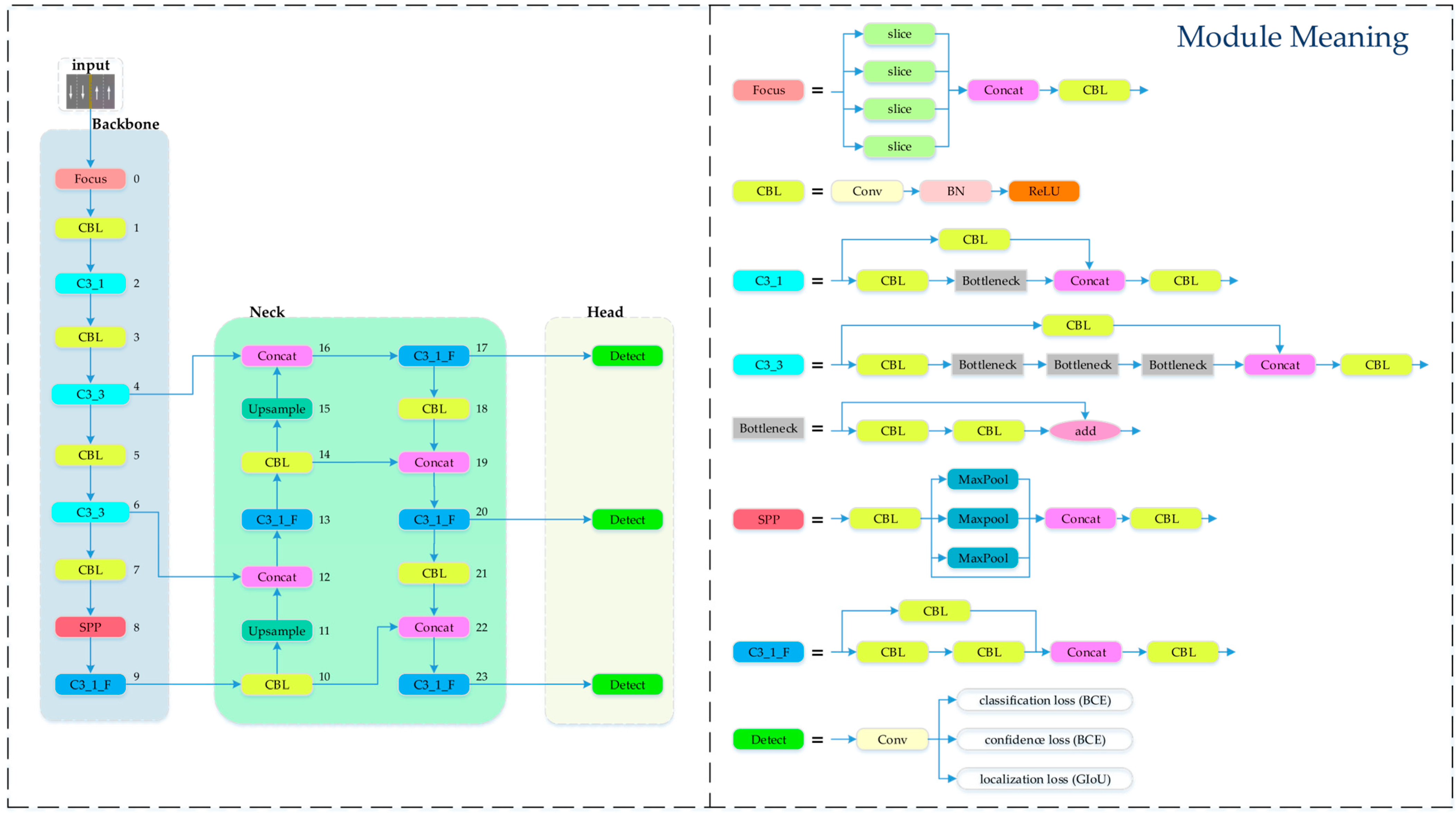
Therefore, this paper proposes a deep learning-based method for detecting the categories of lane lines. Deep learning techniques have powerful learning capabilities and thus have become the dominant approach in machine vision. Girshick proposed a region-based convolutional neural network (R-CNN) [7], a fast region-based convolutional neural network (Fast R-CNN) [8], and a faster region-based convolutional neural network (Faster R-CNN) [9], which were initially applied to object detection tasks. However, these algorithms suffered from slow detection speeds and struggled to meet real-time requirements. Despite their improvement in many works in the literature [10,11,12], the results are still unsatisfactory. The YOLO [13,14,15,16,17,18] series made significant improvements in detection speed. Among them, the YOLOv5 algorithm has been widely used in various object recognition scenarios, with many engineering projects incorporating and improving it.

Musha et al. [19] proposed a lightweight model called CEMLB-YOLO to detect maize leaf blight in complex field environments. The method uses CIPAM attention mechanism to retain key information. After that, feature re-structuring and fusion module is introduced to extract semantic information, and finally MobileBit is added to the feature extraction network. The method achieves an accuracy of 87.5% on the NLB dataset. Abolghasemi et al. [20], based on the improved YOLO model, applied it to the detection of skin cancer. The method adds convolutional layers and residual blocks to the YOLO model and also introduces feature splicing of different layers to achieve multi-scale fusion. Tsoulos et al. [21] used bird image datasets captured in the field to train the YOLOv4 model. Through experiments, it is demonstrated that YOLOv4 can be used for bird detection in the field and has achieved good detection results. Pérez-Patricio et al. [22] detected the behaviour of lambs based on predictive modelling and deep learning. In this regard, a model, an object-tracking algorithm, and a decision tree-based behavioural classifier based on YOLOv4 applied to top-view videos are proposed. Experimentally, the method achieved 99.85% accuracy in detecting lamb activity. He et al. [23] proposed a target recognition algorithm named TF-YOLO based on the improvement of YOLOv3. The method firstly clusters the dataset using K-means++, after which the base model is optimised using the idea of FPN. Through the experimental surface, TF-YOLO can improve the detection accuracy of small targets and achieve the light weight of the network.

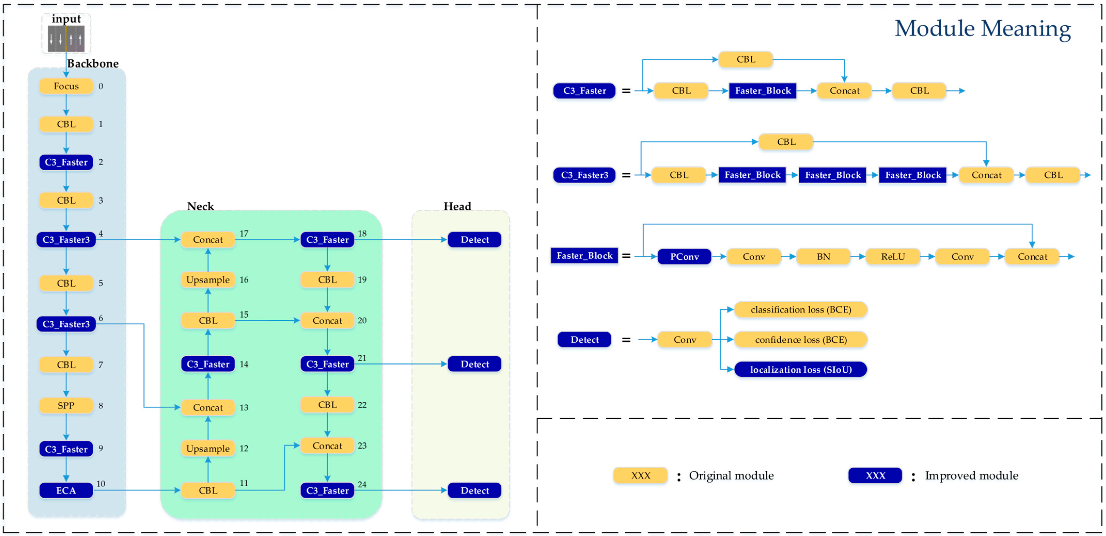
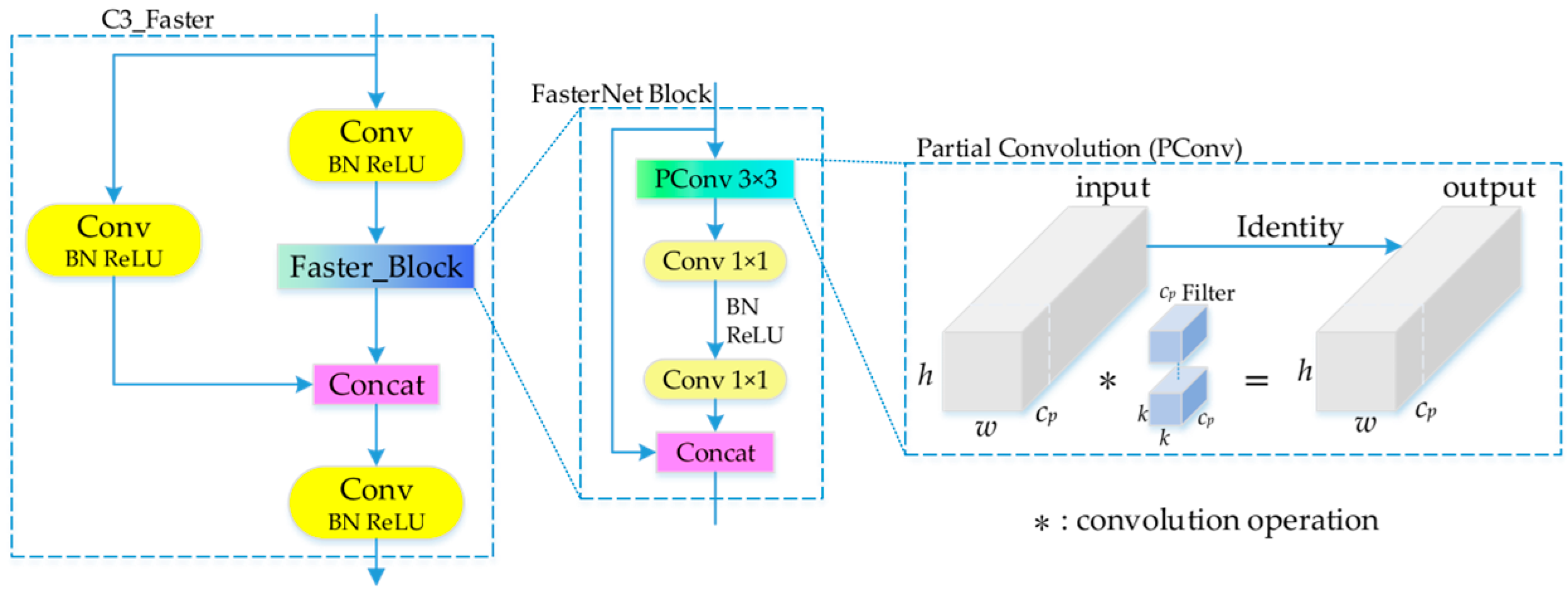
While deep learning techniques have been used in a number of fields, fine-grained methods for recognising lane line type are not yet available. Some deep learning-based lane line detection methods can only singularly go about identifying the shape or colour of a lane line [24]. This is difficult for meeting the requirements of ADAS. In summary, this paper proposes a lane line classification method based on improved YOLOv5. 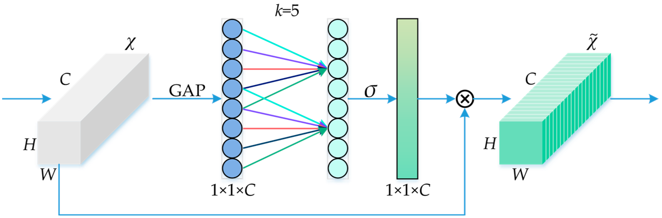The main contributions include incorporating the FasterNet [25] lightweight network into the C3 module of the overall network to achieve parameter reduction and speed improvement. The ECA [26] mechanism is introduced to enhance the model’s feature extraction capability. The SIoU [27] loss function is used instead of the original GIoU [28] loss function to further improve the model’s inference speed and accuracy. Through experiments, it is found that the method in this paper has high accuracy and very fast detection speed. The type of lane lines can be identified even under adverse conditions. This can fully meet the needs of ADAS. It also plays a role in promoting the development of ADAS.

The structure of the rest of this article is as follows. Section 2 outlines the underlying network used in this paper and the strategy for improving the network. Section 3 outlines the experimental setting, the dataset, and the evaluation metrics of the model for this paper. Section 4 analyses the experimental results of the network improved in this paper. Finally, Section 5 summarises the article.

2. Method

2.1. Basic Principles of the YOLOv5 Algorithm

The YOLOv5 algorithm is a representative neural network in the field of deep learning. It belongs to one-stage detection algorithms, which accomplish both object recognition and classification. In one-stage algorithms, the input dataset images are passed through only one network for feature extraction. Anchor frames are used in the last layer for prediction, and the result generated contains both location and category information. In contrast, two-stage detection algorithms requires first generating candidate frames. Based on the candidate frames, the corresponding features are extracted, and a classifier is used to classify the target for each candidate frame. Finally, based on this, bounding box regression is performed on the candidate boxes to determine the target location. Compared to two-stage algorithms, one-stage algorithms have lower accuracy but require less computation, resulting in faster processing speed. Lane line classification is part of the perception module in ADAS, which demands real-time capability. Taking these factors into consideration, the YOLOv5 algorithm is selected for lane line classification.

The YOLOv5 algorithm has four versions: YOLOv5s, YOLOv5m, YOLOv5l, and YOLOv5x, based on different model depths and feature map widths. Among them, YOLOv5s has the smallest model depth and feature map width among all versions, followed by YOLOv5m, YOLOv5l, and YOLOv5x. Specific data are shown in

Table 1. Parameters of different YOLOv5 versions.

Model	Depth Multiple	Width Multiple
YOLOv5s	0.33	0.50
YOLOv5m	0.67	0.75
YOLOv5l	1.00	1.00
YOLOv5x	1.33	1.25

. As the model size increases, the recognition accuracy gradually improves, but the inference speed decreases. According to different tasks and requirements, you can choose the appropriate version to use. For tasks requiring high detection speed, choose YOLOv5s or YOLOv5m. For tasks requiring high accuracy, choose YOLOv5l or YOLOv5x. Considering the real-time requirements of ADAS, this paper selects the YOLOv5s algorithm as the network model for lane line classification.

YOLOv5s consists of the input, backbone network, neck network, and head output, as shown in Figure 1. The input is augmented with mosaic data, adaptive anchor frame computation, and adaptive image scaling. Its main role is to pre-process the dataset images to improve the accuracy and generalisation of the model. The backbone network contains a network of classifiers with good performance, including the C3 module, the CBL module, and the spatial pyramid pooling (SPP) module. It is mainly used to extract feature information from the input image for subsequent object detection tasks. The neck network adopts the FPN [29] + PAN [30] structure. It can enhance the multi-scale semantic representation and localisation ability of the model, and further improve the diversity and robustness of image features. The header output layer is responsible for generating the final object recognition result. This part applies multi-level feature fusion and loss function to improve the detection performance of the model.

2.2. Improved YOLOv5 Algorithm

This paper proposes an improvement scheme for the original YOLOv5s algorithm, which has problems such as low detection accuracy and poor real-time performance. The improved network structure is shown in Figure 2. The improvements are mainly reflected in the following three aspects.

• In the C3 module of the backbone network and neck network, the FasterNet lightweight network is introduced to form the C3_Faster module. This effectively reduces redundant computations and memory access, reducing the model size and accelerating the inference speed.
• The ECA mechanism is introduced at the end of the backbone, which incorporates attention on both channel and spatial dimensions. This significantly enhances the model’s feature extraction capability.
• In the localisation loss function, the SIoU is used instead of the original GIoU function. SIoU takes into account the vector angle between the ground truth box and the predicted box, redefining the penalty metric. This further improves training convergence speed and inference accuracy structure.

2.2.1. FasterNet Lightweight Network

The main idea behind using the FasterNet lightweight network is to achieve model lightweight transformation and faster inference speed while ensuring recognition accuracy. This paper introduces the FasterNet lightweight network into the C3 module of the original YOLOv5 network, forming the C3_Faster module, as shown in Figure 3. The FasterNet block stack is added to each C3 module. The FasterNet block consists of a PConv layer followed by two 1 × 1 convolution layers. To maintain feature diversity and achieve lower latency, normalisation and activation functions are placed between these two convolution layers.

The partial convolution (PConv) layer performs conventional convolution on only some of the input channels to extract spatial features while keeping the rest of the channels unchanged, thus effectively reducing computational redundancy and memory access. For consecutive or regular memory access, the first or last continuous “c_p” channels are treated as representatives of the entire feature map for computation. In general, it is assumed that the input and output feature maps have the same number of channels. The floating-point operations per second (FLOPS) of each PConv can be calculated as

$$h\times w\times k^2\times c_p^2$$

(1)

where h and w represent the length and width of the feature, respectively, c_p represents the number of channels, and k represents the convolution kernel. The FLOPS of the PConv is only 1/16 of the flops of a conventional convolution layer. Additionally, the PConv has a smaller memory access and its data are approximately

$$h\times w\times 2c_p+k^2\times c_p^2\approx h\times w\times 2c_p$$

(2)

which is only 1/4 of a regular convolution layer.

The normalisation layer uses the batch normalisation (BN) [31] layer, which can be fused into its adjacent convolution layer to accelerate the model’s inference speed. The activation layer adopts the rectified linear unit (ReLU) [32] function to reduce runtime and enhance the effectiveness of recognition.

2.2.2. ECA Mechanism

The attention mechanism can be seen as a dynamic weight adjustment process based on input features. In terms of vision, humans can naturally and effectively extract the desired regions in complex scenes through their brains. Inspired by this observation, attention mechanisms have been introduced in computer vision to mimic this aspect of the human visual system.

In this paper, the ECA mechanism is used to implement a non-dimensional reduction local cross-channel interaction strategy using one-dimensional convolution, as shown in Figure 4. This module takes the global average pooling of the feature map for each channel and generates a weight coefficient using a linear layer and sigmoid activation function. The original feature map is then multiplied by this weight coefficient, resulting in a weighted feature map. It requires only a small number of parameters to achieve performance improvement. Avoiding dimensionality reduction is crucial for learning channel attention, so the ECA mechanism enables cross-channel interactions while significantly reducing model complexity and maintaining performance.

Given the aggregated features [C, 1, 1] obtained through the average pooling layer, the ECA mechanism generates channel weights by performing one-dimensional convolution with a kernel size of k, as shown in this equation:

$$\omega =\sigma \left({\mathrm{C}1\mathrm{D}}_k\left(\mathrm{y}\right)\right)$$

(3)

where C1D indicates 1D convolution. The adaptive determination of the kernel size k is based on the mapping of the number of channels C, as shown in this equation:

$$k={\left|\frac{{\log }_{2}C+b}{\gamma }\right|}_{\mathrm{odd}}$$

(4)

where C represents the number of channels. Through ablation experiments, γ is set to 2 and b is set to 1. These parameters are used to adjust the proportion between the number of channels C and the kernel size k. When the number of channels is large, the kernel size k will increase with C. Conversely, when the number of channels is small, the kernel size k will decrease with C. This approach enables effective interaction among different channels, thereby facilitating fusion.

2.2.3. SIoU Loss Function

The detection head of the YOLOv5 algorithm consists of three loss functions: classification loss, confidence loss, and localisation loss. In this paper, the GIoU loss function in the localisation loss is replaced with the SIoU loss function. SIoU takes into account the vector angle between the required regression loss and the matching direction of the ground truth box and the model-predicted box. It redefines the penalty metric, which can accelerate the convergence speed during training and improve the accuracy of inference. The SIoU loss function consists of four cost functions, including angle cost, distance cost, shape cost, and IoU cost.

The schematic diagram of the SIoU loss function calculation scheme is shown in Figure 5. The definitions of each cost function are as follows:

$$①\mathrm{Angle} \cos \mathrm{t}:\Lambda =1-2\ast {\sin }^2\left(\arcsin \left(\frac{c_h}{\sigma }\right)-\frac{\mathsf{\pi }}{4}\right) =\cos \left(2\ast \left(\arcsin \left(\frac{c_h}{\sigma }\right)-\frac{\mathsf{\pi }}{4}\right)\right)$$

(5)

where $\sigma =\sqrt{{\left({\mathrm{B}}_{c_x}^{\mathrm{gt}}-{\mathrm{B}}_{c_x}\right)}^2+{\left({\mathrm{B}}_{c_y}^{\mathrm{gt}}-{\mathrm{B}}_{c_y}\right)}^2}$, and $c_h=\max \left({\mathrm{B}}_{c_y}^{\mathrm{gt}},{\mathrm{B}}_{c_y}\right)-\min \left({\mathrm{B}}_{c_y}^{\mathrm{gt}},{\mathrm{B}}_{c_y}\right)$. $\left({\mathrm{B}}_{c_x}^{\mathrm{gt}},{\mathrm{B}}_{c_y}^{\mathrm{gt}}\right)$ and $\left({\mathrm{B}}_{c_x}{,\mathrm{B}}_{c_y}\right)$ represent the centre coordinates of the true and predicted boxes, respectively.

$$②\mathrm{Distance} \cos \mathrm{t}:\Delta ={\displaystyle \sum _{t=x,y}\left(1-e^{-\gamma {\rho }_t}\right)} =2-e^{-\gamma {\rho }_x}-e^{-\gamma {\rho }_y}$$

(6)

where ${\rho }_x=\left(\frac{{\mathrm{B}}_{c_x}^{\mathrm{gt}}-{\mathrm{B}}_{c_x}}{C_w}\right)$, ${\rho }_y=\left(\frac{{\mathrm{B}}_{c_y}^{\mathrm{gt}}-{\mathrm{B}}_{c_y}}{C_h}\right)$, and $\gamma =2-\Lambda$. C_w and C_h represent the width and height of the minimum enclosing rectangle for the ground truth box and predicted box, respectively.

$$③\mathrm{Shape} \cos \mathrm{t}:\Omega ={{\displaystyle \sum _{t=w,h}\left(1-e^{-w_t}\right)}}^{\theta }={\left(1-e^{-w_w}\right)}^{\theta }+{\left(1-e^{-w_h}\right)}^{\theta }$$

(7)

where $w_w=\frac{\left|w-w^{\mathrm{gt}}\right|}{\max \left(w,w^{\mathrm{gt}}\right)}$ and $w_h=\frac{\left|h-h^{\mathrm{gt}}\right|}{\max \left(h,h^{\mathrm{gt}}\right)}$; w and h represent the width and height of the predicted box, respectively; w_gt and h_gt represent the width and height of the ground truth box, respectively. The parameter “θ” controls the attention given to shape loss. To prevent excessive emphasis on shape loss, which could hinder the movement of the predicted box, the parameter range is constrained to [2,6].

$$④\mathrm{IoU} \cos \mathrm{t}:\mathrm{IoU}=\frac{\left|\mathrm{B}\cap {\mathrm{B}}^{\mathrm{gt}}\right|}{\left|\mathrm{B}\cup {\mathrm{B}}^{\mathrm{gt}}\right|}$$

(8)

where B and B^gt represent the region framed by the model prediction and the region framed by the actual label, respectively.

Based on the calculations mentioned above, the SIoU loss function can be obtained:

$$\mathrm{SIoU}:L_{box}=1-\mathrm{IoU}+\frac{\Delta +\Omega }{2}$$

(9)

3. Experimental Section

3.1. Experimental Environment and Hyperparameters

The software and hardware environment configurations used for algorithm training in this paper are shown in

Table 2. Experimental environment.

Type	Parameter
CPU	Intel(R) Xeon(R) Platinum 8255C CPU @ 2.50 GHz
RAM	45 GB
GPU	NVIDIA RTX3090 GPU with 24 GB of VRAM
VRAM	24 GB
Programming language	Python 3.7
Deep learning framework and dependency library	Pytorch 1.10.2, CUDA 11.6, Cudnn 8.3.2, Numpy 1.19.5, tqdm 4.64.1, tensorboard 2.10.1, OpenCV-Python 4.6.0.66

.

The hyperparameter settings for the algorithm are presented in

Table 3. Hyperparameter settings.

Hyperparameter	Value
Epochs	300
Batch size	16
Image size	640
Optimiser	SGD
Learning rate	0.01
Momentum	0.937

.

3.2. Experimental Dataset

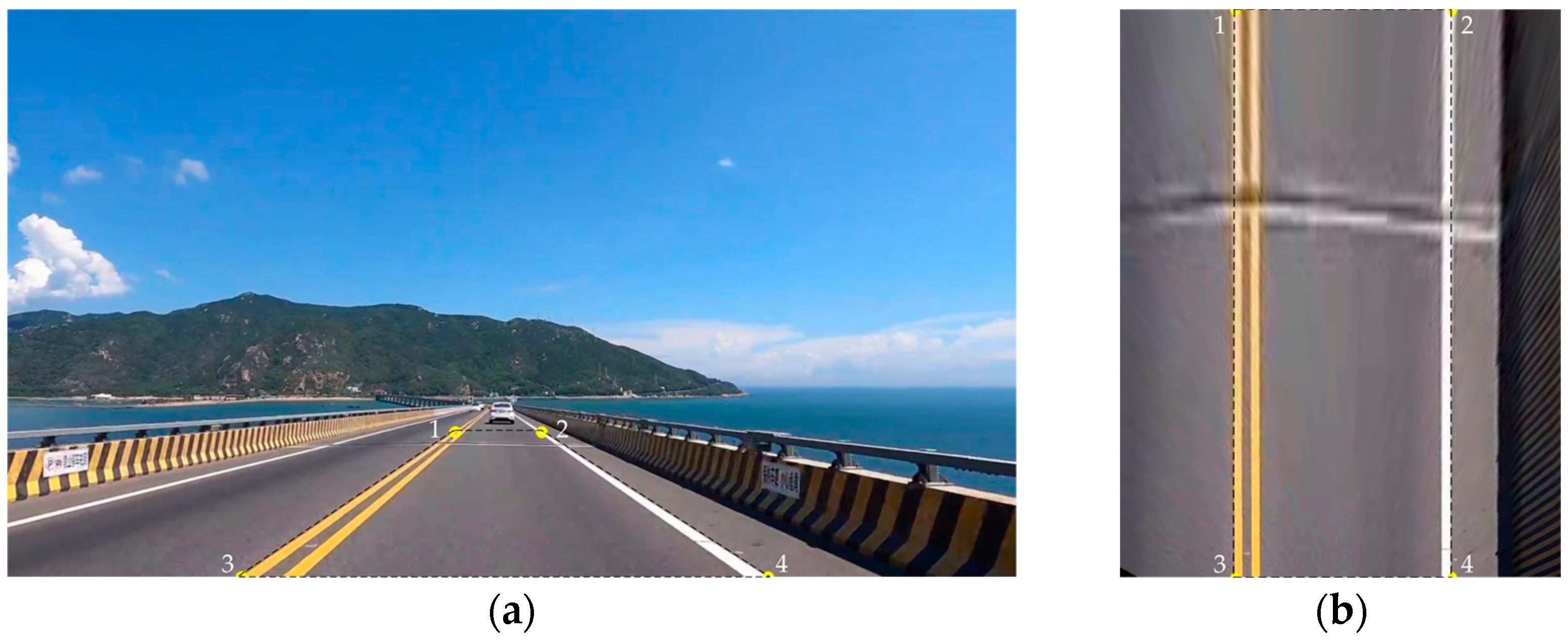
The dataset used for the experiments includes the CULane [33] dataset and custom dataset with inverse perspective transformation. As shown in Figure 6, the road image is transformed using inverse perspective transform to create a bird’s-eye-view road image that reflects the real world. This image shows lane line features more clearly and facilitates feature extraction for the network.

In the inverse perspective transformation, the relationship between the original image and the transformed image can be represented by a 3 × 3 transformation matrix. This matrix is computed based on four corresponding points in the data image, as shown in this equation:

$$\left[\begin{array}{c}{t}_i{x}_i^{\prime }\\ t_i{y}_i^{\prime }\\ t_i\end{array}\right]=map\_matrix\cdot \left[\begin{array}{c}{x}_i\\ y_i\\ 1\end{array}\right]$$

(10)

where map_matrix represents the computed 3 × 3 inverse perspective transformation matrix, and (x_i, y_i) and ($x_i^{\prime }$, $y_i^{\prime }$) represent the coordinates of the input point and the output point, respectively. The value of i ranges from 0 to 3, indicating the corresponding four points. This method allows us to obtain a bird’s-eye view of the road without requiring extensive computational resources. It is a simple operation that only requires processing the region of interest (ROI) containing the lane lines, thereby removing significant amounts of irrelevant information.

According to GB 5768.3-2009 National Standard of China [34], the classification of road traffic markings includes categories such as white dashed lines, white solid lines, yellow dashed lines, yellow solid lines, double white dashed lines, double white solid lines, white dash-solid lines, double yellow solid lines, double yellow dashed lines, yellow dash-solid lines, orange dashed lines, orange solid lines, blue dashed lines, and blue solid lines. Among these, the type of lane markings used to separate traffic flows or restrict vehicle crossings include white dashed lines, white solid lines, yellow dashed lines, yellow solid lines, white dash-solid lines, double yellow solid lines, double yellow dashed lines, and yellow dash-solid lines. The white dash-solid lines and yellow dash-solid lines can be further classified as left-dashed right-solid and left-solid right-dashed based on their position in the driving lane. These lane line types are the targets we need to identify in this paper. The dataset categories are annotated, and the label names are shown in

Table 4. Lane line type data and labels.

Label Name	Lane Line Name	Legend
s_w_i	white dashed line
s_w_f	white solid line
s_y_i	yellow dashed line
s_y_f	yellow solid line
w_lf_ri	white dash-solid line
w_li_rf
d_y_f	double yellow solid line
d_y_i	double yellow dashed line
y_lf_ri	yellow dash-solid line
y_li_rf

.

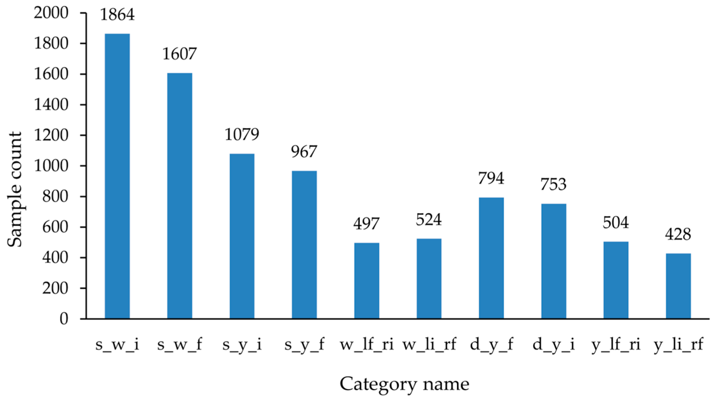
The data images were filtered to exclude road images that do not contain lane lines. Data images with different weather conditions and brightness levels were collected to enhance the model’s generalisation capability. After the filtering process, a total of 5480 images containing lane lines were selected. The dataset was then divided into training, validation, and testing sets in an 8:1:1 ratio.

The sample distribution of training dataset for each type of lane line is shown in Figure 7.

3.3. Evaluation Metrics

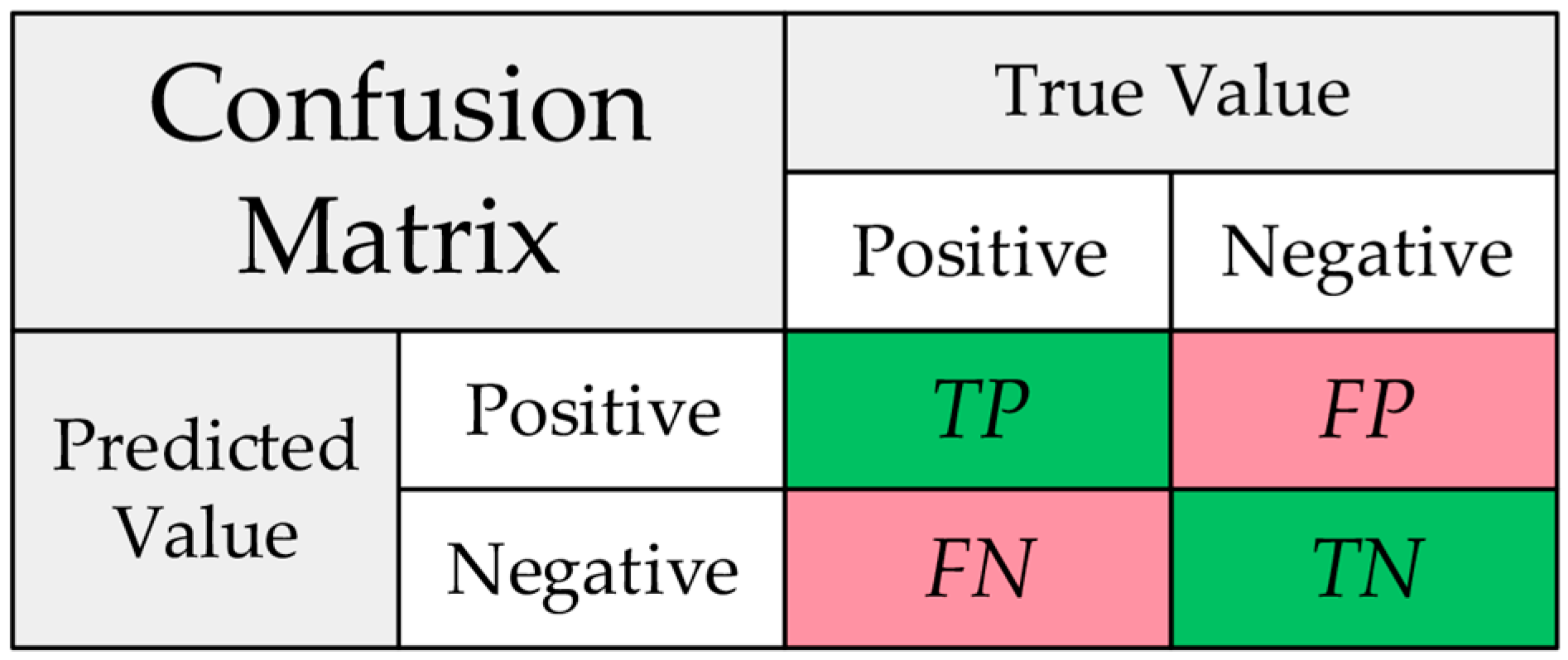
To evaluate the results of lane line category recognition and measure the performance of the trained model, evaluation metrics are used. There are many types of evaluation metrics, but they all rely on a confusion matrix, as shown in Figure 8.

The four values in the confusion matrix are primary indicators: TP (true positive) represents actual positive samples correctly predicted as positive; FN (false negative) represents actual positive samples incorrectly predicted as negative; FP (false positive) represents actual negative samples incorrectly predicted as positive; TN (true negative) represents actual negative samples correctly predicted as negative.

To limit the values of the metrics between 0 and 1, secondary indicators are used to calculate precision and recall. Precision is calculated using the following formula:

$$Precision=\frac{TP}{TP+FP}$$

(11)

Recall is calculated using the following formula:

$$Recall=\frac{TP}{TP+FN}$$

(12)

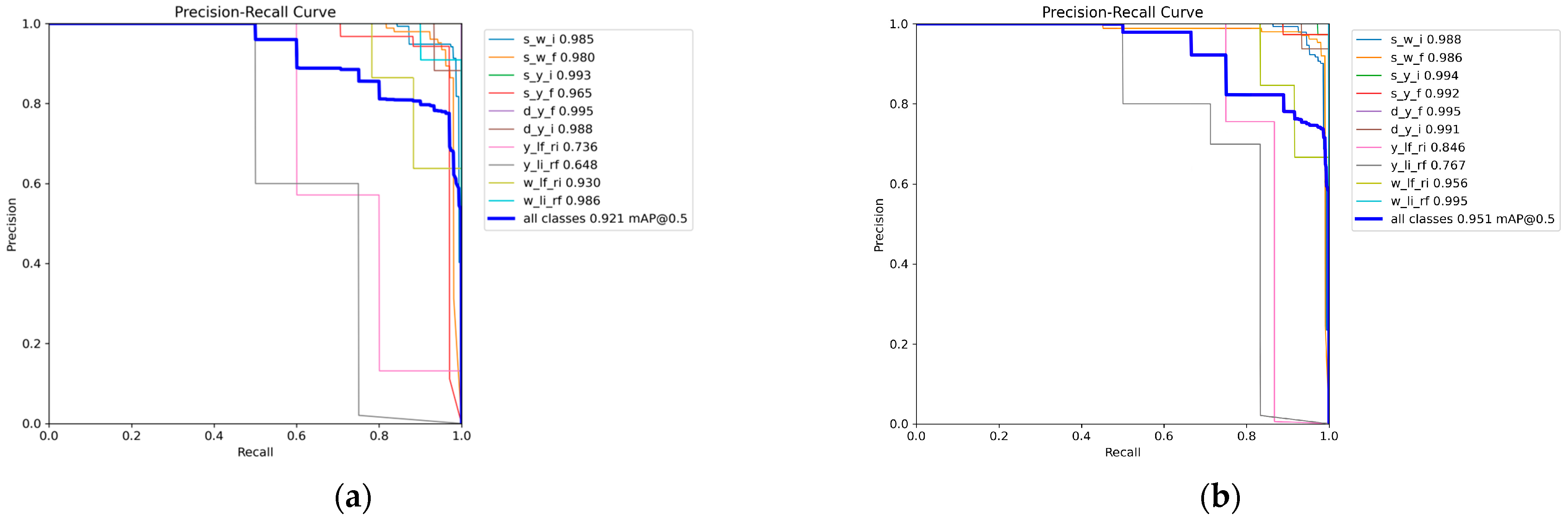
Precision and recall are conflicting measures. When a higher precision is desired, the recall decreases and vice versa. Therefore, this paper uses mAP@0.5 as the evaluation metric for the model. AP represents the accuracy based on the IoU threshold of positive and negative samples, determining the correctness of sample classification based on confidence levels. The AP value is calculated by measuring the area under the precision–recall curve (P-R curve), effectively balancing the conflicting nature of the two indicators. The calculation formula for AP is

$$AP={\displaystyle {\int }_0^{1}P\left(R\right)}\mathrm{d}R$$

(13)

mAP represents the average AP value across all classes and is calculated using the following formula:

$$mAP=\frac{{\displaystyle {\sum }_{i=1}^{k}A{P}_i}}{k}$$

(14)

In this paper, mAP@0.5 is used as the evaluation metric to represent the average AP values when the IoU threshold is set to 0.5.

The complexity of a model can be evaluated by the number of parameters it has, which is mainly related to the overall structure of the model. Parameters represent the total number of trainable parameters in the network model. The larger the number of parameters, the more complex the model structure.

Real-time performance is an important metric for lane line category recognition in ADAS. Frames per second (FPS) is used to evaluate the real-time capability of the model. A higher FPS indicates faster detection speed and better real-time performance, while a lower FPS indicates poorer real-time performance.

4. Result

In order to verify the effectiveness of the improved algorithm, this paper carries out three sets of experiments based on the YOLOv5 network: the comparison experiment of attention mechanisms, the comparison experiment of loss function, and the ablation experiment of the improved algorithm. After that, comparison experiments with other mainstream target recognition algorithms and YOLO series are also set up. Finally, different environments are simulated using grayscale values and peak signal-to-noise ratios to analyse the applicability of the algorithm in real road conditions.

4.1. Comparative Experiment of Attentional Mechanisms

To verify the effectiveness of the ECA mechanism, a comparison was made with other attention mechanisms, including the convolutional block attention module (CBAM) [35] and the squeeze-and-excitation module (SE) [36]. The experimental results are shown in

Table 5. Comparison of results with different attention mechanisms.

Model	mAP@0.5 (%)	Parameters (M)	FPS (frame·s−1)
YOLOv5s	92.1	7.1	91.3
YOLOv5s + CBAM	94.1	7.6	82.6
YOLOv5s + SE	93.7	8.3	79.4
YOLOv5s + ECA	94.3	7.2	84.7

.

From the table, it can be observed that all three attention mechanisms can improve the mAP@0.5 of the model. However, by comparison, it is found that introducing the ECA mechanism has a higher improvement in mAP@0.5 compared to the SE and CBAM mechanisms. It improved 2.2% over the original model.

4.2. Comparison Experiment of Loss Function

Based on the good performance of the ECA module in previous experiments. In this section, the effectiveness of the SIoU loss function is evaluated on this basis. And the training results are compared with the training results of the three loss functions, GIoU, complete intersection over union (CIoU) [37], and efficient intersection over union (EIoU) [38]. The experimental results are shown in

Table 6. Comparison of results using different loss functions.

Model	mAP@0.5 (%)	Parameters (M)	FPS (frame·s−1)
YOLOv5s + ECA + GIoU	94.3	7.2	84.7
YOLOv5s + ECA + CIoU	95.0	7.2	87.7
YOLOv5s + ECA + EIoU	94.8	7.2	89.3
YOLOv5s + ECA + SIoU	95.4	7.2	85.5

.

From the table, it can be observed that using the SIoU loss function outperforms the other three loss functions, effectively improving the model’s mAP@0.5. Compared with the GIoU loss function in the original model, it was increased by 1.1%, and FPS also improved slightly.

4.3. Ablation Experiment

To validate the overall effectiveness of the improved algorithm, a set of ablation experiments were conducted. The experiment included six models with different configurations: ① Original YOLOv5s; ② YOLOv5s + C3_Faster; ③ YOLOv5s + ECA; ④ YOLOv5s + SIoU; ⑤ YOLOv5s + ECA + SIoU; ⑥ YOLOv5s + C3_Faster + ECA + SIoU. The experimental results are shown in

Table 7. Comparison of results from ablation experiments.

YOLOv5s	C3_Faster	ECA	SIoU	mAP@0.5 (%)	Parameters (M)	FPS (frame·s−1)	Volume (MB)
√				92.1	7.1	91.3	13.8
√	√			91.9	5.8	99.0	11.4
√		√		94.3	7.2	84.7	13.9
√			√	93.8	7.1	92.6	13.8
√		√	√	95.4	7.2	85.5	13.9
√	√	√	√	95.1	6.0	95.2	11.7

√: Introduction of the module.

.

From the table, it can be observed that compared to the original model, introducing the FasterNet lightweight network in the C3 module alone speeds up the model’s processing speed and reduces the number of parameters. The introduction of the ECA mechanism and SIoU loss function both improve the model’s mAP@0.5. When the three improvements are introduced simultaneously, the accuracy of the model increases by 3.0%, the FPS increases by 3.9 frame·s⁻¹, the number of parameters decrease by 1.1 M, and the volume decreases by 2.1 MB. In conclusion, the method proposed in this paper has higher robustness and real-time performance in lane line type recognition compared to other methods. Meanwhile, the parameters and volume of the model are effectively reduced.

4.4. Comparative Experiment of Different Algorithms

To demonstrate the good performance of the YOLO algorithm on the task of lane line species recognition, this section cites one two-stage algorithm, Faster R-CNN, and two one-stage algorithms, SSD [39] and RetinaNet [40], as comparison networks. These are the current mainstream target recognition algorithms. These algorithms have been applied by many researchers in various task scenarios. The above algorithms are applied to the lane line pattern recognition dataset for training and testing. And the results of YOLOv5 algorithm are compared with the results of the above algorithms. The results are shown in

Table 8. Comparison of results from different algorithms.

Model	mAP@0.5 (%)	FPS (frame·s−1)	Volume (MB)
Faster R-CNN(Vgg16)	88.1	13.5	522.1
Faster R-CNN(ResNet50)	86.0	6.3	108.5
SSD(Vgg16)	86.7	45.5	95.1
SSD(ResNet50)	82.8	68.9	49.8
SSD(MobileNetv2)	73.1	71.2	18.8
RetinaNet	85.6	53.3	139.9
YOLOv5s	92.1	91.3	13.8
Oure-YOLOv5s	95.1	95.2	11.7

.

As can be seen from the table, the detection speed of Faster R-CNN is too slow and bulky. This is not suitable for application and deployment in ADAS. Compared with Faster R-CNN, the SSD and RetinaNet algorithms improve the detection speed, but the average accuracy is lower, which is still difficult for meeting the needs of ADAS. The YOLOv5 algorithm is superior to the above three algorithms in terms of average accuracy and detection speed. On this basis, the improved YOLOv5 algorithm proposed in this paper has further improved in each performance. This algorithm is fully applicable to the working requirements of ADAS.

4.5. Comparative Experiment of YOLO Series Algorithms

In order to further verify the effectiveness of the improved algorithm, this paper sets up a comparison experiment between different YOLO algorithms. It mainly includes YOLOv3, YOLOv4, and YOLOv5. The experimental results are shown in

Table 9. Comparison of results of different YOLO versions.

Model	mAP@0.5 (%)	Parameters (M)	FPS (frame·s−1)	Volume (MB)
YOLOv3	88.5	61.6	26.5	117.9
YOLOv3-tiny	76.8	8.7	140.8	16.7
YOLOv4	89.5	64.4	24.0	224.6
YOLOv4-tiny	81.5	5.9	128.4	22.6
YOLOv5s	92.1	7.1	91.3	13.8
YOLOv5m	94.4	20.9	41.2	40.3
YOLOv5l	95.5	46.2	25.1	88.6
YOLOv5x	96.7	86.3	13.4	165.2
Ours-YOLOv5s	95.1	6.0	95.2	11.7
Ours-YOLOv5m	95.8	15.8	43.7	30.6
Ours-YOLOv5l	96.1	32.3	26.9	62.1
Ours-YOLOv5x	96.9	57.0	15.3	109.4

.

From the table, it can be seen that although YOLOv3 and YOLOv4 have improved their recognition accuracy compared to the other algorithms listed in the previous section, their detection speeds are still far from adequate. YOLOv3-tiny and YOLOv4-tiny used CSPdarknet53_tiny as the backbone network and improved on the basis of the original network. Although the detection speed has been greatly improved, the detection accuracy has dropped off a cliff. After the improved algorithm in this paper, compared with the original YOLOv5s, YOLOv5m, YOLOv5l, and YOLOv5x, the four different models have different degrees of improvement in detection accuracy and speed. The improved algorithm reduces the parameters and volume of the model. In practical applications, the appropriate detection model can be selected according to the embedded deployment of ADAS.

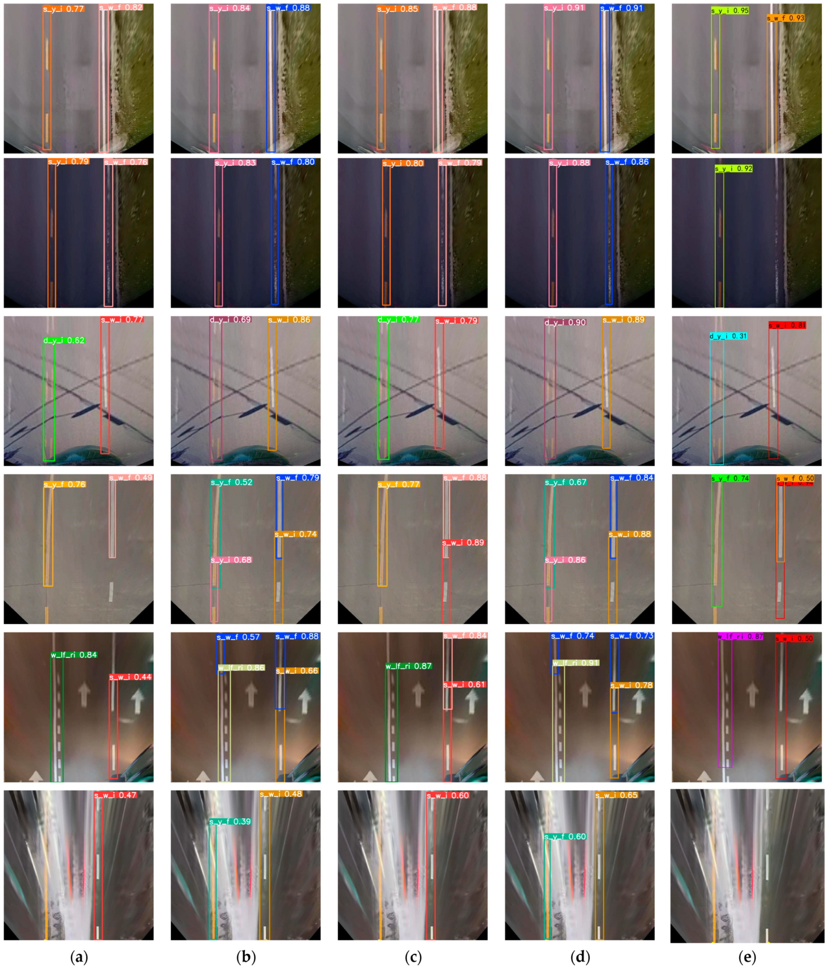
From Figure 9, the improved algorithm has a higher confidence in the recognition of various types of lane lines. Especially in various complex situations, it can effectively avoid leakage or misdetection. This suggests that the improved YOLOv5 algorithm has a wider range of applications and is more suitable for ADAS applications and deployments.

As can be seen in Figure 10, the improved algorithm improves the detection accuracy for all categories of targets to different degrees, especially for the lane line category with more complex features. When using YOLOv5s, the detection of the yellow dash-solid line is poor. However, under our improved algorithm, the detection results of the two types of short yellow dash-solid lines are improved by 11% and 11.9%, respectively, which indicates that our improved strategy has some effect.

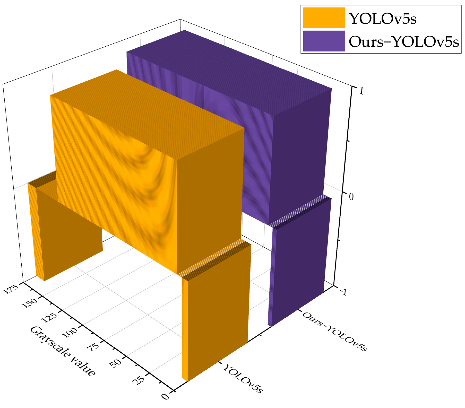
4.6. Analysis of Influence of Light Intensity

In this paper, in order to analyse the applicability of the improved algorithm in different light intensities, different light intensities outdoors are simulated using different levels of contrast and brightness. In order to simulate a real scene, the range of grayscale values is set between 0–175, and the pixels of the pictures in the test set are modified.

Through experiments, the original YOLOv5s algorithm is able to correctly identify lane line type with grayscale values ranging from 10–137, with detection failures in ranges smaller than 6 and larger than 164. The rest of the ranges are false-positive cases, mainly in that yellow lane lines are incorrectly identified as white lane lines. While the improved YOLOv5s algorithm can correctly identify the type of lane line grayscale values ranging between 8–155, less than 4 and greater than 171 are the range of detection failure. The rest of the range are cases of false positives. As shown in Figure 11, where the Z-axis indicates the detection results, 1 indicates accurate recognition, 0 indicates false positive, and −1 indicates recognition failure.

In summary, the method proposed in this paper has a wider detection range for different light intensities compared to the original algorithm.

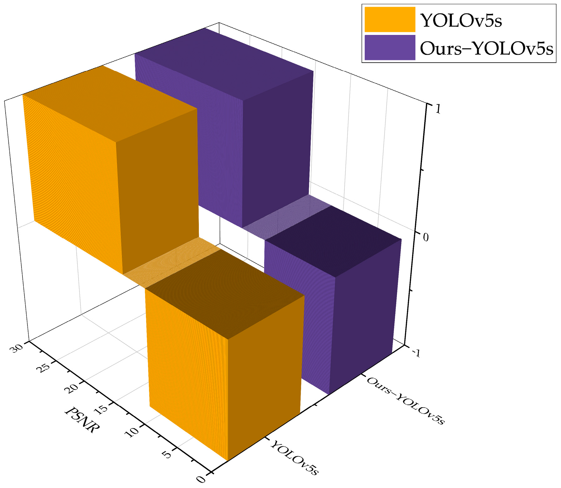
4.7. Analysis of the Influence of Noise

In this paper, in order to analyse the applicability of the improved algorithm in the case of noise interference in different weather, different levels of Gaussian noise are added to the images to simulate rain, snow, or foggy weather. The peak signal-to-noise ratio (PSNR) is utilised to evaluate the quality of the image after adding noise. PSNR is defined based on mean square error (MSE). The definition of MSE is

$$\mathrm{MSE}=\frac{1}{mn}{\displaystyle \sum _{i=0}^{m-1}{\displaystyle \sum _{j=0}^{n-1}{\left[I\left(i,j\right)-K(i,j)\right]}^2}}$$

(15)

where m × n represents the size of the image, and I(i,j) and K(i,j) represent the pixels of the original image and the pixels of the noisy image, respectively.

Then, PSNR can be defined as

$$\mathrm{PSNR}=20{\log }_{10}\left(\frac{MA{X}_I}{\sqrt{MSE}}\right)$$

(16)

where MAX_I is the maximum pixel value of the image.

Through experiments, under the influence of noise, the original YOLOv5s algorithm correctly recognises lane line type in the range greater than 15.2 dB, while the range of recognition failure is less than 11.8 dB. The rest of the ranges are false positives or false negatives. While the improved algorithm correctly recognises the lane line type in the range greater than 13.3 dB, the range of recognition failure is less than 9.8 dB. The rest of the ranges are false positives or false negatives. As shown in Figure 12, where the Z-axis indicates the detection results, 1 indicates accurate recognition, 0 indicates false positive or false negative, and −1 indicates recognition failure.

In summary, compared to the original algorithm, the method proposed in this paper is able to accurately recognise lane line type in more severe weather.

5. Conclusions

To ensure the accuracy and real-time performance of lane line category recognition, this paper proposes an improved YOLOv5 algorithm. Through experiments, the following conclusions have been drawn:

• Introducing FasterNet into the C3 module of the backbone and necking networks can speed up the inference speed of the model and reduce the calculation parameters.
• Introducing the ECA mechanism into the backbone network can significantly improve the recognition accuracy of the model.
• The use of SIoU loss function can further improve the accuracy of the model and speed up the inference speed to some extent.

According to the experimental results on the dataset, the improved YOLOv5 model achieves the mAP@0.5 of 95.1% and the FPS of 95.2 frames·s⁻¹ in the test. This meets the requirements for accuracy and real-time performance in lane line type recognition. Moreover, the parameters and the volume of the model are only 6.0 M and 11.7 MB, respectively. It also has a wider detection range than the original YOLOv5 algorithm in different environments. Therefore, the proposed method can be effectively applied to lane line category recognition and has practical significance for application in ADAS.

References

1. Wippelhauser, A.; Edelmayer, A.; Bokor, L. A Declarative Application Framework for Evaluating Advanced V2X-Based ADAS Solutions. Appl. Sci. 2023, 13, 1392. [Google Scholar] [CrossRef]
2. Zou, Y.; Ding, L.; Zhang, H.; Zhu, T.; Wu, L. Vehicle Acceleration Prediction Based on Machine Learning Models and Driving Behavior Analysis. Appl. Sci. 2022, 12, 5259. [Google Scholar] [CrossRef]
3. Ulrich, L.; Nonis, F.; Vezzetti, E.; Moos, S.; Caruso, G.; Shi, Y.; Marcolin, F. Can ADAS Distract Driver’s Attention? An RGB-D Camera and Deep Learning-Based Analysis. Appl. Sci. 2021, 11, 11587. [Google Scholar] [CrossRef]
4. Park, C.; Chung, S.; Lee, H. Vehicle-in-the-Loop in Global Coordinates for Advanced Driver Assistance System. Appl. Sci. 2020, 10, 2645. [Google Scholar] [CrossRef]
5. Ma, C.; Xie, M. A Method for Lane Detection Based on Color Clustering. In Proceedings of the 2010 Third International Conference on Knowledge Discovery and Data Mining, Phuket, Thailand, 9–10 January 2010; pp. 200–203. [Google Scholar] [CrossRef]
6. Rui, R. Lane line detection technology based on machine vision. In Proceedings of the 2022 4th International Conference on Artificial Intelligence and Advanced Manufacturing (AIAM), Hamburg, Germany, 7–9 October 2022; pp. 562–566. [Google Scholar] [CrossRef]
7. Girshick, R.; Donahue, J.; Darrell, T.; Malik, J. Rich Feature Hierarchies for Accurate Object Detection and Semantic Segmentation. In Proceedings of the IEEE Conference on Computer Vision and Pattern Recognition, Columbus, OH, USA, 23–28 June 2014; pp. 580–587. [Google Scholar] [CrossRef]
8. Girshick, R. Fast R-CNN. arXiv 2015, arXiv:1504.08083. [Google Scholar]
9. Ren, S.; He, K.; Girshick, R.; Sun, J. Faster R-CNN: Towards Real-Time Object Detection with Region Proposal Networks. IEEE Trans. Pattern Anal. Mach. Intell. 2017, 39, 1137–1149. [Google Scholar] [CrossRef]
10. Xiang, J.; Shi, H.; Huang, X.; Chen, D. Improving Graphite Ore Grade Identification with a Novel FRCNN-PGR Method Based on Deep Learning. Appl. Sci. 2023, 13, 5179. [Google Scholar] [CrossRef]
11. Wang, H.; Xiao, N. Underwater Object Detection Method Based on Improved Faster RCNN. Appl. Sci. 2023, 13, 2746. [Google Scholar] [CrossRef]
12. Liang, B.; Wang, Z.; Si, L.; Wei, D.; Gu, J.; Dai, J. A Novel Pressure Relief Hole Recognition Method of Drilling Robot Based on SinGAN and Improved Faster R-CNN. Appl. Sci. 2023, 13, 513. [Google Scholar] [CrossRef]
13. Redmon, J.; Divvala, S.; Girshick, R.; Farhadi, A. You Only Look Once: Unified, Real-Time Object Detection. In Proceedings of the 2016 IEEE Conference on Computer Vision and Pattern Recognition (CVPR), Las Vegas, NV, USA, 27–30 June 2016; pp. 779–788. [Google Scholar] [CrossRef]
14. Redmon, J.; Farhadi, A. YOLO9000: Better, Faster, Stronger. In Proceedings of the 2017 IEEE Conference on Computer Vision and Pattern Recognition (CVPR), Honolulu, HI, USA, 21–26 July 2017; pp. 6517–6525. [Google Scholar] [CrossRef]
15. Redmon, J.; Farhadi, A. YOLOv3: An Incremental Improvement. arXiv 2018, arXiv:1804.02767. [Google Scholar]
16. Bochkovskiy, A.; Wang, C.-Y.; Liao, H.-Y.M. YOLOv4: Optimal Speed and Accuracy of Object Detection. arXiv 2020, arXiv:2004.10934. [Google Scholar]
17. Wang, C.-Y.; Bochkovskiy, A.; Liao, H.-Y.M. Scaled-YOLOv4: Scaling Cross Stage Partial Network. arXiv 2020, arXiv:2011.08036. [Google Scholar]
18. YOLOv5. 2021. Available online: https://github.com/ultralytics/yolov5 (accessed on 10 December 2022).
19. Leng, S.; Musha, Y.; Yang, Y.; Feng, G. CEMLB-YOLO: Efficient Detection Model of Maize Leaf Blight in Complex Field Environments. Appl. Sci. 2023, 13, 9285. [Google Scholar] [CrossRef]
20. Singh, S.K.; Abolghasemi, V.; Anisi, M.H. Fuzzy Logic with Deep Learning for Detection of Skin Cancer. Appl. Sci. 2023, 13, 8927. [Google Scholar] [CrossRef]
21. Mpouziotas, D.; Karvelis, P.; Tsoulos, I.; Stylios, C. Automated Wildlife Bird Detection from Drone Footage Using Computer Vision Techniques. Appl. Sci. 2023, 13, 7787. [Google Scholar] [CrossRef]
22. González-Baldizón, Y.; Pérez-Patricio, M.; Camas-Anzueto, J.L.; Rodríguez-Elías, O.M.; Escobar-Gómez, E.N.; Vazquez-Delgado, H.D.; Guzman-Rabasa, J.A.; Fragoso-Mandujano, J.A. Lamb Behaviors Analysis Using a Predictive CNN Model and a Single Camera. Appl. Sci. 2022, 12, 4712. [Google Scholar] [CrossRef]
23. He, W.; Huang, Z.; Wei, Z.; Li, C.; Guo, B. TF-YOLO: An Improved Incremental Network for Real-Time Object Detection. Appl. Sci. 2019, 9, 3225. [Google Scholar] [CrossRef]
24. Farag, W.; Saleh, Z. Road Lane-Lines Detection in Real-Time for Advanced Driving Assistance Systems. In Proceedings of the 2018 International Conference on Innovation and Intelligence for Informatics, Computing, and Technologies (3ICT), Sakhier, Bahrain, 18–20 November 2018; pp. 1–8. [Google Scholar] [CrossRef]
25. Chen, J.; Kao, S.H.; He, H.; Zhuo, W.; Wen, S.; Lee, C.H.; Chan, S.H.G. Run, Don’t Walk: Chasing Higher FLOPS for Faster Neural Networks. In Proceedings of the 2023 IEEE/CVF Conference on Computer Vision and Pattern Recognition (CVPR), Vancouver, BC, Canada, 17–24 June 2023; pp. 12021–12031. [Google Scholar] [CrossRef]
26. Wang, Q.; Wu, B.; Zhu, P.; Li, P.; Zuo, W.; Hu, Q. ECA-Net: Efficient Channel Attention for Deep Convolutional Neural Networks. In Proceedings of the 2020 IEEE/CVF Conference on Computer Vision and Pattern Recognition (CVPR), Seattle, WA, USA, 13–19 June 2020; pp. 11531–11539. [Google Scholar] [CrossRef]
27. Gevorgyan, Z. SIoU Loss: More Powerful Learning for Bounding Box Regression. arXiv 2022, arXiv:2205.12740. [Google Scholar]
28. Rezatofighi, H.; Tsoi, N.; Gwak, J.; Sadeghian, A.; Reid, I.; Savarese, S. Generalized Intersection Over Union: A Metric and a Loss for Bounding Box Regression. In Proceedings of the 2019 IEEE/CVF Conference on Computer Vision and Pattern Recognition (CVPR), Long Beach, CA, USA, 15–20 June 2019; pp. 658–666. [Google Scholar] [CrossRef]
29. Lin, T.-Y.; Dollár, P.; Girshick, R.; He, K.; Hariharan, B.; Belongie, S. Feature pyramid networks for object detection. In Proceedings of the IEEE Conference on Computer Vision and Pattern Recognition, Honolulu, HI, USA, 21–26 July 2017; pp. 2117–2125. [Google Scholar] [CrossRef]
30. Liu, S.; Qi, L.; Qin, H.; Shi, J.; Jia, J. Path Aggregation Network for Instance Segmentation. In Proceedings of the 2018 IEEE/CVF Conference on Computer Vision and Pattern Recognition (CVPR), Salt Lake City, UT, USA, 18–23 June 2018; pp. 8759–8768. [Google Scholar] [CrossRef]
31. Ioffe, S.; Szegedy, C. Batch Normalization: Accelerating Deep Network Training by Reducing Internal Covariate Shift. In Proceedings of the 32nd International Conference on Machine Learning, Lile, France, 6–11 July 2015; pp. 448–456. [Google Scholar]
32. Krizhevsky, A.; Sutskever, I.; Hinton, G.E. ImageNet classification with deep convolutional neural networks. Commun. ACM 2017, 60, 84–90. [Google Scholar] [CrossRef]
33. Pan, X.; Shi, J.; Luo, P.; Wang, X.; Tang, X. Spatial as deep: Spatial cnn for traffic scene understanding. In Proceedings of the AAAI Conference on Artificial Intelligence, New Orleans, LA, USA, 2–7 February 2018; pp. 7276–7283. [Google Scholar] [CrossRef]
34. State General Administration of the People’s Republic of China for Quality Supervision and Inspection. Quarantine and National Standard of the People’s Republic of China. In Road Traffic Signs and Markings: Part 3, Road Traffic Markings; Standards Press of China: Beijing, China, 2009. [Google Scholar]
35. Woo, S.; Park, J.; Lee, J.-Y.; Kweon, I.S. CBAM: Convolutional Block Attention Module. In Proceedings of the Computer Vision—ECCV 2018: 15th European Conference, Munich, Germany, 8–14 September 2018; pp. 3–19. [Google Scholar] [CrossRef]
36. Hu, J.; Shen, L.; Sun, G. Squeeze-and-Excitation Networks. In Proceedings of the 2018 IEEE/CVF Conference on Computer Vision and Pattern Recognition, Salt Lake City, UT, USA, 18–23 June 2018; pp. 7132–7141. [Google Scholar] [CrossRef]
37. Zheng, Z.; Wang, P.; Liu, W.; Li, J.; Ye, R.; Ren, D. Distance-IoU Loss: Faster and Better Learning for Bounding Box Regression. arXiv 2019, arXiv:1911.08287. [Google Scholar] [CrossRef]
38. Zhang, Y.-F.; Ren, W.; Zhang, Z.; Jia, Z.; Wang, L.; Tan, T. Focal and Efficient IOU Loss for Accurate Bounding Box Regression. arXiv 2021, arXiv:2101.08158. [Google Scholar] [CrossRef]
39. Liu, W.; Anguelov, D.; Erhan, D.; Szegedy, C.; Reed, S.; Fu, C.-Y.; Berg, A.C. SSD: Single Shot MultiBox Detector. In European Conference on Computer Vision; Springer: Cham, Switzerland, 2016; pp. 21–37. [Google Scholar] [CrossRef]
40. Lin, T.-Y.; Goyal, P.; Girshick, R.; He, K.; Dollár, P. Focal Loss for Dense Object Detection. In Proceedings of the 2017 IEEE International Conference on Computer Vision (ICCV), Venice, Italy, 22–29 October 2017; pp. 2999–3007. [Google Scholar] [CrossRef]
Figure 1. YOLOv5s network structure.
Applsci 13 10537 g001
Figure 2. Improved YOLOv5s network structure.
Applsci 13 10537 g002
Figure 3. C3_Faster module.
Applsci 13 10537 g003
Figure 4. ECA mechanism.
Applsci 13 10537 g004
Figure 5. SIoU loss function calculation scheme diagram.
Applsci 13 10537 g005
Figure 6. Inverse perspective transformation: (a) original image; (b) after perspective transformation.
Applsci 13 10537 g006
Figure 7. Sample size of all types of lane lines.
Applsci 13 10537 g007
Figure 8. Confusion matrix.
Applsci 13 10537 g008
Figure 9. Results of different YOLO algorithms: (a) YOLOv5s; (b) Ours-YOLOv5s; (c) YOLOv5x; (d) Ours-YOLOv5x; (e)YOLOv4-tiny.
Applsci 13 10537 g009
Figure 10. Comparison of models mAP@0.5: (a) YOLOv5s; (b) Ours-YOLOv5s.
Applsci 13 10537 g010
Figure 11. Comparison of the algorithm before and after improvement under different light intensities.
Applsci 13 10537 g011
Figure 12. Comparison of the algorithm before and after improvement under different levels of noise.
Applsci 13 10537 g012