Article

A Multi-Fidelity Successive Response Surface Method for Crashworthiness Optimization Problems

Institute of Vehicle Concepts, German Aerospace Center (DLR), Pfaffenwaldring 38-40, 70569 Stuttgart, Germany
*
Author to whom correspondence should be addressed.
Appl. Sci. 2023, 13(20), 11452; https://doi.org/10.3390/app132011452
Submission received: 6 September 2023 / Revised: 3 October 2023 / Accepted: 11 October 2023 / Published: 19 October 2023
(This article belongs to the Special Issue Structural Optimization Methods and Applications)

Abstract

:
Due to the high computational burden and the high non-linearity of the responses, crashworthiness optimizations are notoriously hard-to-solve challenges. Among various approaches, methods like the Successive Response Surface Method (SRSM) have stood out for their efficiency in enhancing baseline designs within a few iterations. However, these methods have limitations that restrict their application. Their minimum iterative resampling required is often computationally prohibitive. Furthermore, surrogate models are conventionally constructed using Polynomial Response Surface (PRS), a method that is poorly versatile, prone to overfitting, and incapable of quantifying uncertainty. Furthermore, the lack of continuity between successive response surfaces results in suboptimal predictions. This paper introduces the Multi-Fidelity Successive Response Surface (MF-SRS), a Gaussian process-based method, which leverages a non-linear multi-fidelity approach for more accurate and efficient predictions compared to SRSM. After initial testing on synthetic problems, this method is applied to a real-world crashworthiness task: optimizing a bumper cross member and crash box system. The results, benchmarked against SRSM and the Gaussian Process Successive Response Surface (GP-SRS)—a single-fidelity Gaussian process-driven extension of SRSM—show that MF-SRS offers distinct advantages. Specifically, it improves upon the specific energy absorbed optimum value achieved by SRSM by 14%, revealing its potential for future applications.

1. Introduction

At present, the automotive industry is mainly facing two pivotal challenges. The first is the growing importance of road and vehicle safety, which has raised legislative requirements and forced the inclusion of more effective protection systems in vehicles. The second challenge is the rising interest in environmental sustainability and energy transition, which is driving the automotive industry toward higher lightweighting standards, aiming to reduce fuel and battery consumption. In response to these dual challenges, substantial efforts are being made to develop vehicles that are both crashworthy and lightweight, thereby addressing these seemingly contradictory issues at the same time [1].
Over the past decades, the widespread usage of surrogate models, often called metamodels, has fundamentally transformed the approach to complex real-world optimization challenges. These methods, introduced as metamodeling techniques by Sacks et al. nearly 35 years ago [2], have evolved into Metamodel-Based Optimization (MBO), a highly effective strategy for tackling complex black-box “expensive-to-evaluate” functions [3].
This category of functions is particularly prevalent in engineering applications, which are typically underpinned by time-intensive numerical simulations, such as Finite Element Analysis (FEA) and Computational Fluid Dynamics (CFD). These simulations require large computational resources, often monopolizing high-performance computing architectures for hours or even full days [4].
To cope with this issue, surrogate models have emerged as an innovative solution to reduce the vast number of function evaluations required, hence optimizing resource utilization. These models operate as an abstraction of an underlying phenomenon, generating a “model of the model” as referred to by Kleijnen [5]. Surrogate modeling operates by utilizing a set of sampling evaluations. Typically, this process begins with the design space being sampled through Design of Experiment (DoE) techniques. Subsequent numerical simulations at these sampled points are executed and results are used to fit surrogate models over the variable domain [6].
A broad spectrum of metamodeling techniques have been advanced over recent years to aid complex engineering designs that are reliant on simulation-based methods. These include Gaussian Process (GP) [7], Polynomial Response Surface (PRS) [8,9], Support Vector Regression (SVR) [10], Radial Basis Function (RBF) [11], and Neural Network (NN) [12,13]. In the specific context of optimizing crashworthiness problems, PRS, RBF, and GP stand out as the most commonly used and most successful metamodels [14,15].
Alongside regression methods, various global search strategies can be useful in attempting to identify an optimal global solution in crashworthiness optimization. Given the highly non-linearity of these problems, which commonly results in the presence of multiple local minima, methodologies such as Genetic Algorithms (GAs) [16], Evolutionary Algorithms (EAs) [17,18], and Simulated Annealing (SA) [19] are particularly suitable, but they often come with a high computational cost that might be unaffordable. In contrast, gradient-based methods are generally not recommended, particularly for the optimization of frontal collisions, as they exhibit increased sensitivity to bifurcations compared to lateral impacts. However, these methods may prove useful as local search strategies for refining the solution identified by a global optimization algorithm.
Regardless of the regression model considered, the use of global response surfaces is generally discouraged due to the high non-linearity of crash load cases. In contrast, an iterative approach based on the successive construction of response surfaces is recommended, especially when the optimum approaches regions of the variable domain with very high gradients or even discontinuities. This approach, commonly known as the Successive Response Surface Method (SRSM), has been shown to be effective in crashworthiness applications, as demonstrated by the research of Stander et al. and Kurtaran et al. [20,21,22].
Although SRSM has proven capable of identifying the optimal region for various crashworthiness problems, its application has some limitations. First, SRSM relies on iterative resampling, which could be a practical challenge since crashworthiness simulations are very time-consuming. Another potential drawback is the lack of continuity between successive approximations, making it difficult to incorporate information from previous iterations [14,23]. Finally, to our current understanding, the method does not seem well suited for integrating valuable data derived from response evaluations of lower fidelity models. These models, which are comparatively cheaper to evaluate, are often available or can be generated through automated process chains. The effectiveness of such models has been shown in the work of Acar et al. [24].
This paper proposes an approach that further enhances the SRSM and aims to overcome most of its existing limitations. The main contributions of this research are the following:
  • We extended the SRSM to achieve qualitatively superior optima and potentially improve its computational efficiency. This is accomplished by leveraging GP, adaptive sampling techniques, and multi-fidelity metamodeling.
  • Unlike conventional multi-fidelity methods (e.g., basic co-kriging), our approach is based on a method able to effectively handle complex non-linear correlations between different fidelities. We also quickly show how this method benefits from parallel job scheduling on a High-Performance Computer (HPC), enhancing its overall efficiency.
The organization of this paper unfolds as follows. In Section 2, we briefly outline a common iterative process used to optimize crashworthiness problems and provide the necessary mathematical notation. Then, in Section 3, we review the key steps of the sequential response surface methodology. Section 4 then provides a brief overview of multi-fidelity metamodeling based on GPs and touches on its potential applications, in which we distinguish between linear and non-linear multi-fidelity approaches and emphasize the superiority of the latter through a selection of pedagogical examples. This paper continues in Section 5, where we present the workflow of our extension of SRSM based on multi-fidelity metamodeling. In Section 6, we test the proposed approach on a set of multi-fidelity benchmark functions, in addition to a crashworthiness use case. Finally, in Section 7, we outline the conclusions and consider potential future research directions.

2. Crashworthiness Optimization: Problem Formulation

Describing a generic crashworthiness design optimization problem using appropriate mathematical notation is relatively straightforward. Assuming that continuous design variables are to be handled in a single objective-constrained problem, we can mathematically formulate the problem as follows:
min x   f ( x )
    subject to g j ( x ) 0 , j = 1 , , n c
    x i l x i x u l , i = 1 , , d ,
where x R d is the vector of the d design variables, x i l and x i u denote the physical lower and upper bounds on these variables, f is the objective function, and g i with j = 1 , , n c is the jth of the n c constraint functions necessary to set the inequality constraints. Note that both the objective and constraint functions map from the d-dimensional real space to the real numbers, so that f : R d R and g i : R d R , respectively. The goal is to find the optimal x o p t R d , the vector that minimizes the response of the objective function f.

3. Successive Response Surface

Due to the high computational burden and the challenge of globally capturing the non-linearities within the variable domain, the problem, as formulated above, is not yet ready for resolution. The SRSM can navigate us toward a more feasible formulation for such a problem by employing two main adjustments. Initially, the “expensive-to-evaluate” response functions associated with FEA simulations are substituted with the response surface models. Specifically, f and g j are replaced with f ^ and g j ^ respectively, such that f ^ : R d R and g i ^ : R d R . These surrogate models are nothing but regression models constructed on an initial dataset of n p observations, commonly referred to as the Design of Experiment (DoE): D = { ( x p , y p ) | p = 1 , , n p } .
Many authors have used Polynomial Response Surface models as a simple but effective way of generating a surrogate model [22,25,26]. The function is given for a general quadratic polynomial surface approximation:
y p = β 0 + i = 1 d β i x p i + i = 1 d k = 1 d β i k x p i x p k + ε p p = 1 , , n p ,
where x p are the design points used to train the model, y p are the associated evaluated response values, β i are the constants to be determined, and ε p includes both the bias errors and random errors. The minimum number of numerical simulations, denoted as n p , m i n , required to construct a given approximation depends on the number of design variables. For instance, in the case of a quadratic approximation, n p , m i n = ( d + 1 ) ( d + 2 ) / 2 . The D-optimal sampling is frequently employed to explore the variable domain. For a deeper understanding of the PSR and D-optimal criterion, we recommend readers refer to the work of Myers and Montgomery [8].
Moreover, we substitute the original optimization problem with a succession of less complex and smaller problems. Ideally, these subproblems should be located in a subregion of the variable domain and should still provide the same optimal solution to the original problem. We can formulate the kth subproblem by readjusting Equations (1)–(3) as follows:
min x     f ^ ( k ) ( x )
  subject to g j ^ ( k ) ( x ) 0 , j = 1 , , n c
            x i l ( k ) x i x u l ( k ) , i = 1 , , d
where x i l ( k ) x i l , x i u ( k ) x i u ,
where x i l ( k ) and x i l ( k ) define the kth subregion, called the Region of Interest (RoI) by some authors [27,28].
The domain of the variables can be translated and narrowed by adjusting the bounds of each variable. In this way, the focus of optimization can be shifted to only the new simplified domain of interest. Several heuristic schemes using different measures to evaluate the accuracy of the metamodel have been proposed and used to automate the so-called “panning and zooming“ strategy. In this article, we briefly introduce the bounds adjustment scheme, which has been successfully used to solve a variety of crashworthiness optimization problems [20,21,29]. As shown in Figure 1, the Ω k + 1 subproblem is centered on the optimal design of the Ω k subproblem, i.e., x o p t ( k ) . Moreover, the size of the Ω k + 1 subregion is a fraction of the Ω k subregion. This reduction in the feature domain along a generic ith variable is determined by the fraction parameter λ i , which is computed as follows:
λ i ( k + 1 ) = η + ( γ η ) | x i , o p t ( k ) x i u ( k ) + x i l ( k ) 2 | x i u ( k ) x i l ( k ) 2 .
From Equation (9), it is quite clear that λ i ( k + 1 ) is equal to γ when the optimum is located at the lower and upper bounds. This extreme case results in pure panning, i.e., the pure translation of the RoI, when γ = 1 . Conversely, when the optimum lies at the midpoint between x i l ( k ) and x i u ( k ) , λ i ( k + 1 ) is equal to η , resulting in pure zooming or domain shrinkage. It is quite clear that η and γ represent the upper and lower boundary values, respectively, of the fraction parameter λ i .
The maximum value of λ i ( k + 1 ) , represented by λ ( k + 1 ) = max λ i ( k + 1 ) for ( i = 1 , , n ) , is selected as the fraction to be applied across all design variables. This choice preserves the aspect ratio of the design region throughout the iterative process. Using the fraction parameter value λ ( k + 1 ) , we can establish the upper and lower bounds of the ith design variable for the ( k + 1 ) th subregion as follows:
x i l ( k + 1 ) = x i , o p t ( k ) 1 2 λ ( k + 1 ) ( x i u ( k ) x i l ( k ) )
x i u ( k + 1 ) = x i , o p t ( k ) + 1 2 λ ( k + 1 ) ( x i u ( k ) x i l ( k ) ) .

4. Multi-Fidelity Metamodeling

Multi-fidelity modeling techniques are increasingly gaining momentum in the design optimization field, offering a viable solution to reduce the computational cost of high-fidelity response evaluations without compromising accurate metamodel predictions. Even though these techniques may be of a different nature, being based on either linear regression or neural networks, the most common building block of multi-fidelity schemes is GP regression [30,31]. GPs are well-suited to many MF-metamodel methods due to their ability to capture highly non-linear responses in as few functions as possible, which is the reason this study focuses on GP methods.
This section begins with an overview of the Gaussian Process, which is essential for understanding the multi-fidelity approach discussed in this paper. Then, both linear and non-linear multi-fidelity methodologies are described, highlighting their importance, challenges, and solutions for integrating different levels of fidelity.

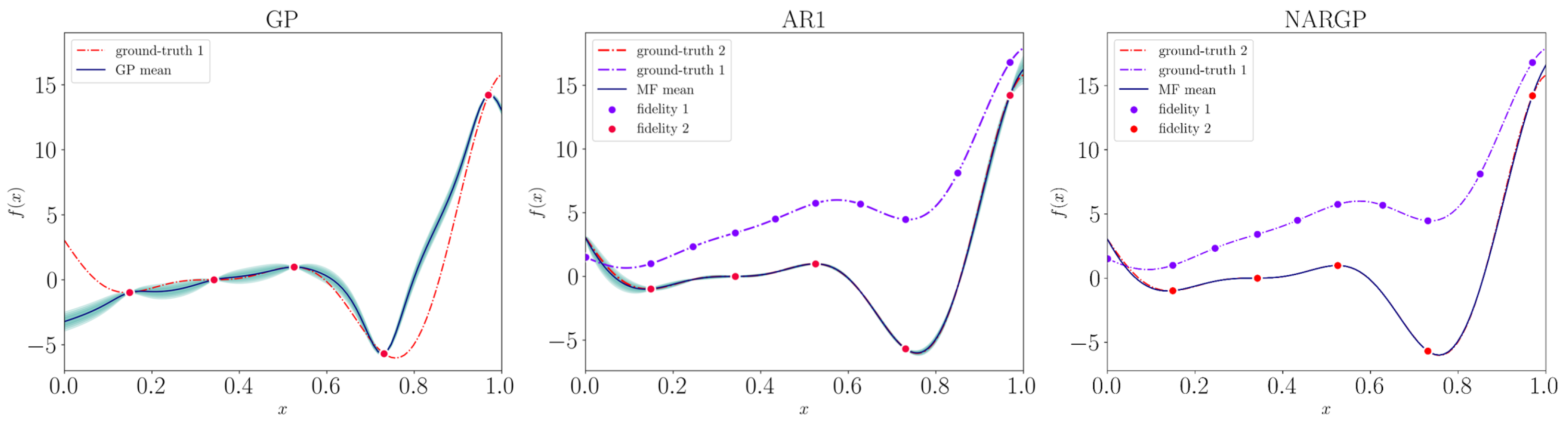
4.1. Background on Gaussian Process

Within the context of black-box expensive-to-evaluate functions, a common goal is to discern the connection between the design variables and a generic black-box function f. This task can be accomplished by initially retrieving a dataset D of input and output observation pairs (for the sake of clarity, we recall that D = { ( x p , y p ) | p = 1 , , n p } = { x , y } ) and then fitting a regression model to the collected observations. Before conditioning on such observations, a GP is defined by its mean function and kernel function (or covariance function):
f ( x ) G P ( μ ( x ) , k ( x i , x j ) ) .
It is common practice to assume that, before conditioning GP on the observations, the mean function is zero across the variable domain, especially since uncertainty about the mean can be accommodated by including an additional term in the kernel [32]. As a result, the structure that a GP can capture is entirely dictated by its covariance function k. This function, which depends on a vector of hyperparameters θ , yields the positive-definite symmetric covariance matrix K R n p × n p . By maximizing the log-marginal likelihood (Equation (13)), it is possible to calculate vector θ :
log p ( D | θ ) = 1 2 y T K 1 y 1 2 log | K | n 2 log 2 π .
Once the hyperparameters are identified, it is possible to infer the posterior distribution by conditioning the joint Gaussian distribution to make predictions on unseen data:
p ( f | x , D , θ ) N ( f | μ ( x ) , σ 2 ( x ) )
μ ( x ) = k n p K 1 y
σ 2 ( x ) = k k n K 1 k n T ,
where x refers to a new given input, f to its prediction, k = k ( x , x ) , and k n = [ k ( x , x 1 ) , , k ( x , x n p ) ] . The posterior mean μ and its related uncertainty, namely the posterior variance σ 2 , can be, therefore, employed to make predictions. For more details on the conditioning of the Gaussian distribution and some examples of covariance functions, we suggest that the reader refer to the work of Rasmussen and Williams [7].

4.2. Linear Multi-Fidelity Metamodeling

In this section, we briefly present a common linear multi-fidelity technique used in engineering disciplines to integrate computational models of varying fidelity (accuracy) to make predictions. This autoregressive scheme was proposed by Kennedy and O’Hagan in 2000 [30], commonly referred to as AR1, and is still widely viewed as a reference point. Although most practical problems involve only two fidelities, we generalize the problem by assuming that we have s levels of information sources available. Therefore, for a generic level t, we define y t ( x t ) to be the output of a given input x t R d . We can then, for each level, group inputs and outputs into a generic database D t = { x t , y t } by ordering the data by increasing fidelity, i.e., t = 1 , , s . In other words, y 1 is the output of the least accurate model, while y s is the output of the most accurate model. That being said, we present the autoregressive scheme of Kenny and O’Hagan in Equation (17):
f t ( x ) = ρ · f t 1 ( x ) + δ t ( x ) .
In Equation (17), ρ serves as a scaling factor to denote the magnitude of correlation among different fidelity outputs, δ t ( x ) is a GP with mean μ δ t and covariance function k t , f t ( x ) , and f t 1 ( x ) are the GPs predicting data at fidelity level t and t 1 , respectively. This linear autoregressive scheme relies on the Markov property, asserting that when the closest point f t 1 ( x ) is known, no further information about f t ( x ) can be gained from any other model output f t 1 ( x ) [33]:
cov { f t ( x ) , f t 1 ( x ) | f t 1 ( x ) } = 0 x x .

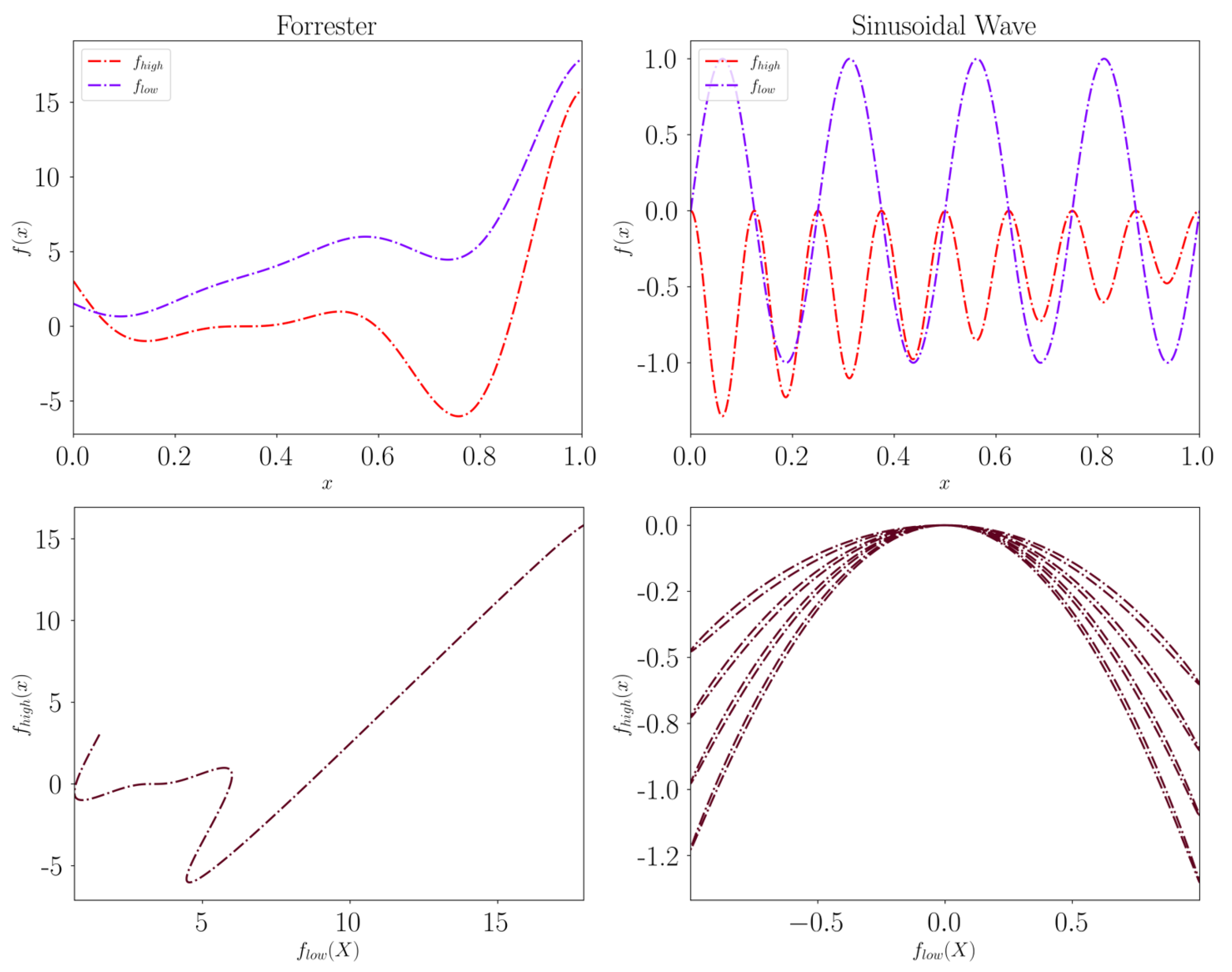
4.3. Non-Linear Multi-Fidelity Metamodeling

Although Kennedy and O’Hagan’s scheme has already been proven successful in the literature [34,35], there are cases that are very common in realistic modeling scenarios, where cross-correlations between models of different fidelity, while very informative, show a more complex pattern than a simple linear correlation. In such a case, a linear autoregressive scheme might work well only in narrow ranges of the input parameters, but would not be able to learn a more comprehensive non-linear correlation in the global domain. With this in mind, we briefly introduce the non-linear autoregressive multi-fidelity GP regression (NARGP) algorithm introduced by Perdikaris et al. [36], which aims to extend the Kennedy and O’Hagan scheme to more complex non-linear and space-dependent correlations. We assume the design datasets to have a nested structure, such as D 1 D 2 , , D s , and we generalize the scheme of Equation (17):
f t ( x ) = z t 1 · f t 1 ( x ) + δ t ( x )
where the mapping between a low model and its higher fidelity counterpart is denoted by the unknown function z t 1 . To enable flexible and non-linear multi-fidelity algorithms, a GP prior is assigned to z. Since f t 1 is also assigned a GP prior, the posterior distribution of f t , because of the functional composition of two priors, is no longer Gaussian.
The generalization outlined in Equation (19) does not come without implications in terms of computational cost and implementation complexity. This is mainly because of the need to use variational Bayesian methods to approximate intractable integrals. Therefore, to favor an algorithmic complexity closer to that of GP regression, Perdikaris et al. proposed a reformulation of the generalized scheme in which the GP prior f t 1 is replaced by the GP posterior of the first inference level f t 1 :
f t ( x ) = g t ( x , f t 1 ( x ) )
where g t is assigned the prior of Equations (21) and (22):
f ( x ) G P ( f t | 0 , k t ; θ t )
k t g = k t ρ ( x , x ; θ t ρ ) · k t f ( f t 1 ( x ) , f t 1 ( x ) ; θ t f ) + k t δ ( x , x ; θ t δ ) ,
where k t ρ , k t f , and k t δ are squared exponential anisotropic kernel functions based on Automatic Relevance Determination (ARD) weights (for additional details, please refer to [7]) and θ t ρ , θ t f , θ t δ represent their hyperparameters. With this scheme, it is possible to infer the high fidelity response through g t by projecting the lower fidelity posterior onto a latent manifold of dimension d + 1 .
The lowest fidelity level of the proposed recursive scheme is still a common GP regressor with kernel function k 1 ( x , x , θ 1 ) . Therefore, its posterior distribution is still Gaussian. However, as for all the other levels, the predictions have to be made given a test point ( x , f t 1 ( x ) ) . Therefore, for t 2 , the posterior distribution is no longer Gaussian and is defined by the following integral:
p ( f t ( x ) ) = X p ( f t ( x , f t 1 ( x ) ) | y t , x t , x ) p ( f t 1 ( x ) ) d x .
Bear in mind that solving the integral of Equation (23) is commonly performed by a recursive Monte Carlo approach [36].

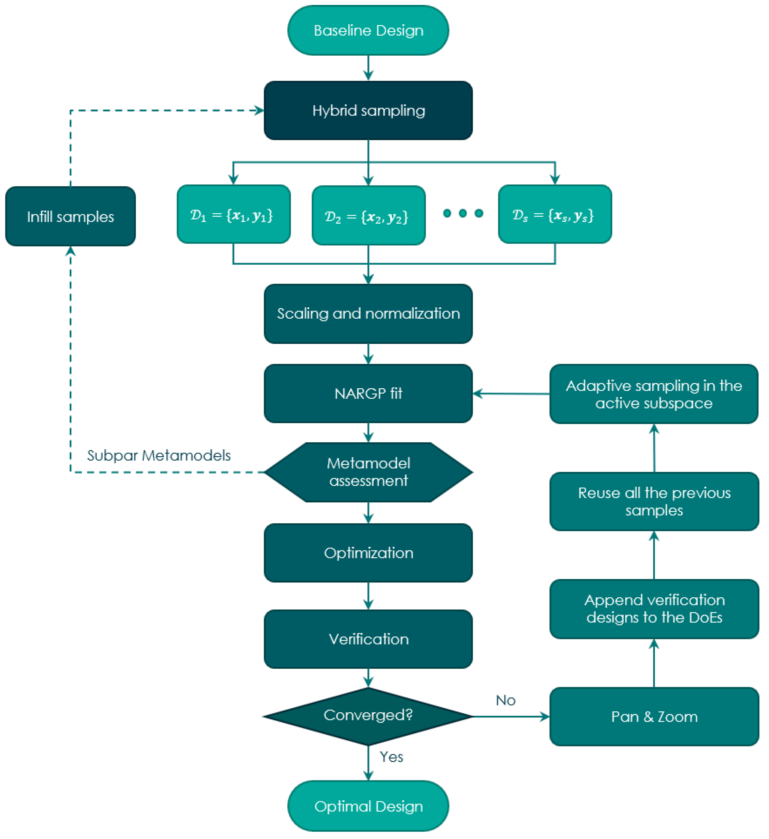
5. Multi-Fidelity Successive Response Surface

As mentioned in the introduction, it is quite clear that the SRSM method has some limitations that limit its application to specific real-world scenarios. In this section, we introduce our improved version of SRSM, tailored for multi-fidelity crashworthiness problems, which we will refer to as the Multi-Fidelity Successive Response Surface (MF-SRS). We will provide an overview of the main workflow and then discuss its key components, highlighting the improvements over the traditional approach.
The general workflow of the MF-SRS approach is shown in Figure 2. The first step is to formulate the optimization problem as described in Section 2. Therefore, it is necessary to define the d design variables with their respective bounds, the objective function, and any n c constraint functions with associated thresholds. Next, we can start the variable domain exploration phase using a hybrid sampling strategy. In this phase, we start with an Optimal Latin Hypercube Design (OLHD) to set the highest fidelity DoE, D s . Samples of lower fidelity are distributed by sequential sampling to gather information about areas left unexplored by the OLHD.
After generating the datasets for each fidelity level and computing their respective responses, the datasets D 1 , , D s undergo preprocessing, which includes scaling of input variables and normalizing the response values. These pre-processed datasets are then fed into the NARGP model, creating a metamodel for each response function. The accuracy of these metamodels is assessed using a cross-validation-based error procedure. If the metamodels do not meet user-defined accuracy targets, infill algorithms can be optionally employed to add more samples. Within the original variable domain, an initial solution is extracted using Metamodel-Based Optimization with an evolutionary algorithm. The identified optimum is verified using Finite Element Analysis (FEA) simulations with the obtained optimal design variables to measure any deviations from the initial prediction. This result is incorporated into the respective DoEs and serves as the center of the RoI for the subsequent iteration. After adjusting the range of variables using the pan-and-zoom method, new exploratory samples are added to the RoI based on the reused samples. The metamodels are then updated with this augmented data. The process iterates until a convergence criterion is met or until a predefined maximum iteration limit is reached.
The following subsections describe the main steps of the MF-SRS framework, starting with sampling strategies. It then explores multi-fidelity response surfaces and sample reuse, RoI adjustments, and appropriate optimization approaches, and concludes with a discussion of the convergence criteria.

5.1. Adaptive Sampling: OLHD and MIPT

Since it is assumed that no a priori information is available about the nature of the response functions, the first stage of the workflow is necessarily a step of pure exploration of the variable domain. In this sampling step, we distribute samples according to a “hybrid” sampling strategy. The highest fidelity points are distributed according to a scheme of pre-optimized Latin Hypercube Designs [37]. As demonstrated by the work of Crombecq et al. [38], these datasets have been optimized for several hours in order to maximize their projective- and space-filling properties. Please note that space-filling properties refer to the ability of a design to uniformly cover the domain of interest, ensuring that the entire input space is adequately represented without leaving large gaps. A dataset with good projective properties, instead, ensures that if we consider only a subset of its dimensions (i.e., we project the design onto a lower dimensional space), the resulting dataset still has desirable space-filling properties in that lower dimensional space. Therefore, unlike the statistical factorial experimental designs commonly used in the SRSM [20], pre-optimized Latin hypercubes allow extracting as much information as possible from each individual sample while avoiding space-near points and repetitive values. We use the database developed by Dam et al. [37], available at [39]. Although this database is extensive, it has its limitations; it only provides datasets for specific combinations of a number of samples and design variables. If the required DoE is not available in this database, we rely on the translational propagation algorithm of Viana et al. to quickly generate Optimal or Near-Optimal Latin Hypercube Designs [40].
Once the highest fidelity DoE is generated, we employ a sequential sampling strategy to build all the remaining lower-fidelity designs.
For this purpose, we use a Monte Carlo method originally developed by Crombeq et al. [38] and extended by Lualdi et al. [6]: mc-inter-proj-th (MIPT). Starting from a pre-existing design, this method is able to add samples with unit granularity, ensuring an optimal trade-off between space-filling and projective properties. As shown in Figure 3, by using the OLHD points, the MIPT algorithm is able to construct an optimal second layer of samples of lower fidelity. This process is repeated iteratively if more than two levels of fidelity are required. Please see Appendix A for more details on the formulation of the MIPT algorithm. The versatility of this algorithm allows us to apply the same adaptive sampling logic across iterative steps. Unlike one-shot sampling methods, such as LHDs, the MIPT method enables the inheritance and reutilization of samples used in previous iterations. This feature is critical in crashworthiness optimization, both to extract the full potential of each individual FEM simulation and to avoid running unnecessarily expensive crashworthiness simulations.
To conclude on the topic of sampling, it is important to emphasize that the MIPT samples are introduced in a purely exploratory fashion, independent of the response function values. While this approach may seem less than optimal at first, it remains one of the most robust and effective strategies, especially when dealing with multiple response functions. Balancing different functions within the same domain can pose challenging problems.

5.2. Multi-Fidelity Response Surface and Sample Reuse

To achieve maximum performance from the regression model, it is essential to pre-process the data obtained from the DoEs. By leveling out the differences in absolute values that may exist, both in the different ranges of the input variables and in the response evaluations associated with different black-box functions, it is possible to avoid unwanted biases and distortions in the metamodel. Therefore, we scale the input variables to a unit hypercube Ω 0 = [ 0 , 1 ] d and standardize the response values to obtain new distributions with the unit mean and zero variance.
The scaled and normalized values of the designs are fed into the NARGP algorithm to infer a posterior distribution of each response function, as explained in Section 4.3. In addition to the regression model and data fusion approach, another significant difference from the original SRSM method is the selection of points for metamodel training. Given the significant computational effort involved in a passive safety FEM analysis, it is imperative to utilize all the information gained from previous iterations. Therefore, in the MF-SRS method, we retain points from previous iterations, both inside and outside the RoI. This strategy ensures a metamodel with a more reliable global trend, allowing us to use fewer points in each iteration for further exploration of the RoI. Refer to Figure 4 for a visualization of how the RoI and the addition of new samples evolve from the initial domain. Please note that both the number of samples and the zoom have been magnified for clarity.
Note that it is always good practice to evaluate the accuracy of the metamodels at the end of the training phase and to add any samples if the reliability of the prediction is poor. Some authors recommend using an additional 10–30% of the initial samples as test points to evaluate the accuracy of the metamodel alone [41]. Given the enormous computational cost this would imply, in the context of crashworthiness optimization, our approach is based on the guidelines of Loeppky et al. [42] for choosing a sufficiently representative initial number of samples (rule n p = 10 · d ) and the leave-one-out cross-validation approach presented by Viana et al. This method evaluates the quality of metamodels without necessitating additional FEM simulations. For an in-depth understanding, readers can refer to [40].

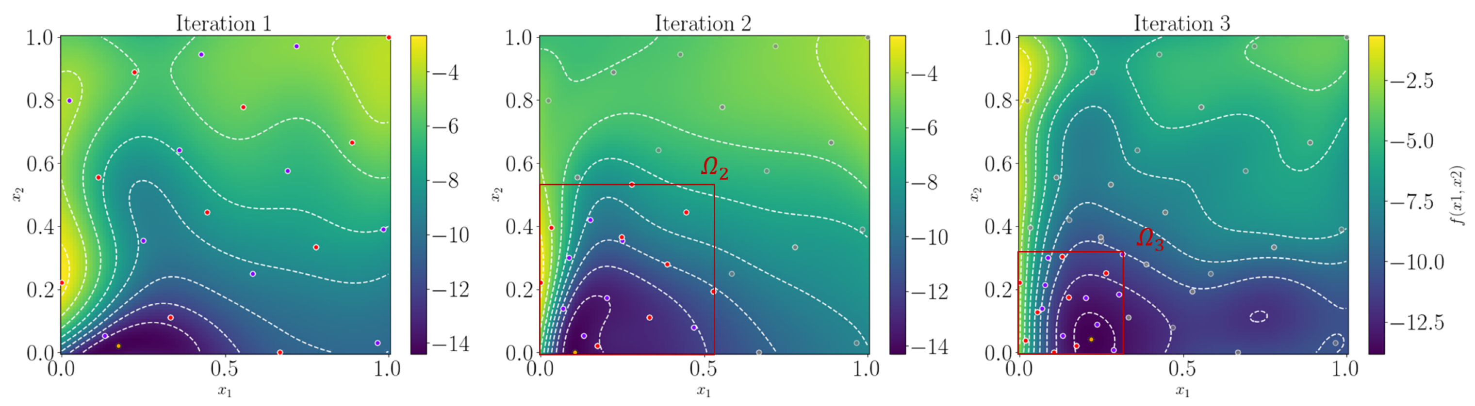
5.3. Adjustment of the RoI

Regarding the definition of the boundaries of the new Region of Interest, we stick to the original algorithm already presented in Equations (9)–(11). As previously discussed, while the boundaries of the new RoI at a given iteration do not define the limits of the metamodel limits, they do set the boundaries for both the optimization algorithm and iterative resampling. Unless otherwise stated, in this article, we will use η = 0.6 and γ = 0.9 as defaults.

5.4. Optimization Approach: Differential Evolution, Trust Region, and Verification Step

Design optimization for expensive-to-evaluate engineering applications involves finding the best set of design variables that meet specific objectives while navigating through a demanding computational environment. Hence, the challenge is to identify the maximum of such costly objective functions with the minimum number of sequential queries, thus reducing time and cost [43].
Numerous single-objective optimization methods have been developed to date, encompassing both local and global optimization techniques. Typically, selecting the right optimization algorithm is crucial for locating the optimum, especially when surface response models are not in use. Yet, as Duddeck pointed out [15], when Metamodel-Based Optimization approaches are employed, the selection of the optimization algorithm becomes less critical if the surrogate models accurately capture the physical properties. This statement highlights the importance of accurate metamodeling for effective optimization of complex engineering design problems.
Our proposed optimization strategy employs a hybrid approach. Initially, we leverage a probability-based global optimization algorithm to rapidly identify an optimal point. Subsequently, using this point as a starting reference, a local method refines the solution. This secondary step ensures that potential local enhancements are duly captured and not overlooked. The Differential Evolution (DE) algorithm is selected as the global optimization method in our approach due to its remarkable convergence properties, capability to address non-linear constraints, adaptability for parallelization, and straightforward implementation. This stochastic global search algorithm excels in managing non-differentiable, non-linear, and multi-modal objective functions. Furthermore, its efficacy is validated in prior studies on structural optimization applications [44,45,46]. In our implementation, we chose a population size of 25, a crossover probability of 0.7, and allowed the differential weight to range from 0.5 to 1 (dithering is employed). These parameter values are based on average values as reported in the tests by Storn et al. [47]. It is important to note that while these parameter choices play a role in the optimization process, they are not of primary importance in determining the optimization result in our context. The accuracy of the metamodel is of greater importance in influencing the final results. Based on our experience, the Covariance Matrix Adaptation Evolution Strategy (CMA-ES) could be a compelling global method, delivering a performance comparable to the DE algorithm. For detailed information on DE and CMA-ES, please refer to [47,48,49], respectively. As a local optimization method, our choice falls on the Trust Region, a popular gradient-based optimization algorithm well suited for non-linear problems. Its use is primarily motivated by the need to manage the quality of the model approximation in non-linear optimization. The basic idea is to iteratively refine an estimate of the optimum based on local information. Like other local optimization methods, Trust Region methods are sensitive to the starting point. If the function has multiple local optima, the method is expected to converge to a different optimum depending on where you start [50]. Therefore, its use must be combined with a global optimization method, such as DE.
In our approach, a local optimization is performed starting from each member of the last population of the DE algorithm. Since optimization on metamodels is very fast compared to the computational burden of a function evaluation, we adopt a DE population size of 20 and we repeat the entire optimization process (global and local optimization) 10 times.
Verification serves as the final step of the optimization phase. The optimal solution derived from the metamodel is validated through an FEA to confirm the accuracy of the metamodel’s prediction compared to the actual ground truth value.

5.5. Convergence Criteria

We use two stopping criteria to determine if the problem has achieved convergence: the maximum number of iterations and the Average Relative Function Tolerance (ARFT). The process is halted when either of these criteria are satisfied. The maximum number of iterations is determined by the user, based on the specific problem at hand. The ARFT formula, inspired by the criterion presented by Querin et al. [51], is provided below:
A R F T k = 1 n A R F T i = 0 n A R F T | f ( x o p t ( k + 1 i ) ) f ( x o p t ( k i ) ) | | f ( x o p t ( k i ) ) | + ϵ .
Here, n A R F T denotes the number of pairs of successive iterations under consideration, and ϵ is a very small number introduced to prevent division by zero when f ( x o p t ( k i ) ) equals zero. Convergence is achieved when A R F T drops below a specified threshold ϵ f :
A R F T k < ϵ f .
By default, we set ϵ = 10 8 and ϵ f = 0.01 . This ensures that the optimization will stop if the average relative change in the objective function over the last three iterations is less than 1%. Unless otherwise stated, in this paper, we will use n A R F T = 4.

6. Results and Discussion

In this chapter, we evaluate the effectiveness of MF-SRS through a series of experiments on both synthetic problems and a real-world engineering challenge. We begin with a visual illustration of two well-known problems from the literature to demonstrate the robustness of a multi-fidelity regression model capable of capturing both linear and non-linear correlations. We continue with optimization tests on multi-fidelity benchmark functions to compare the convergence of the SRSM with the MF-SRS. We conclude with a comprehensive section dedicated to the design optimization of a vehicle front structure subsystem, focusing specifically on a crash box and a bumper cross member. Finally, we briefly analyze a possible integration of a parallel job submission on an HPC.

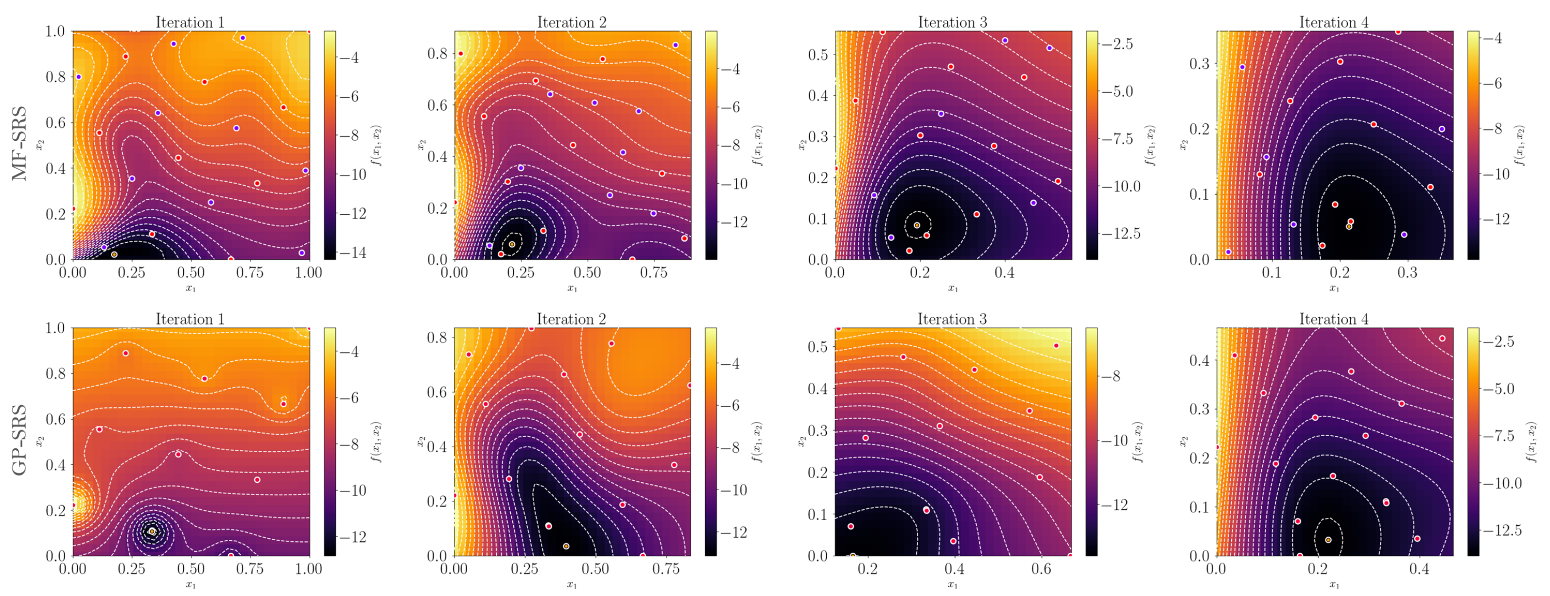
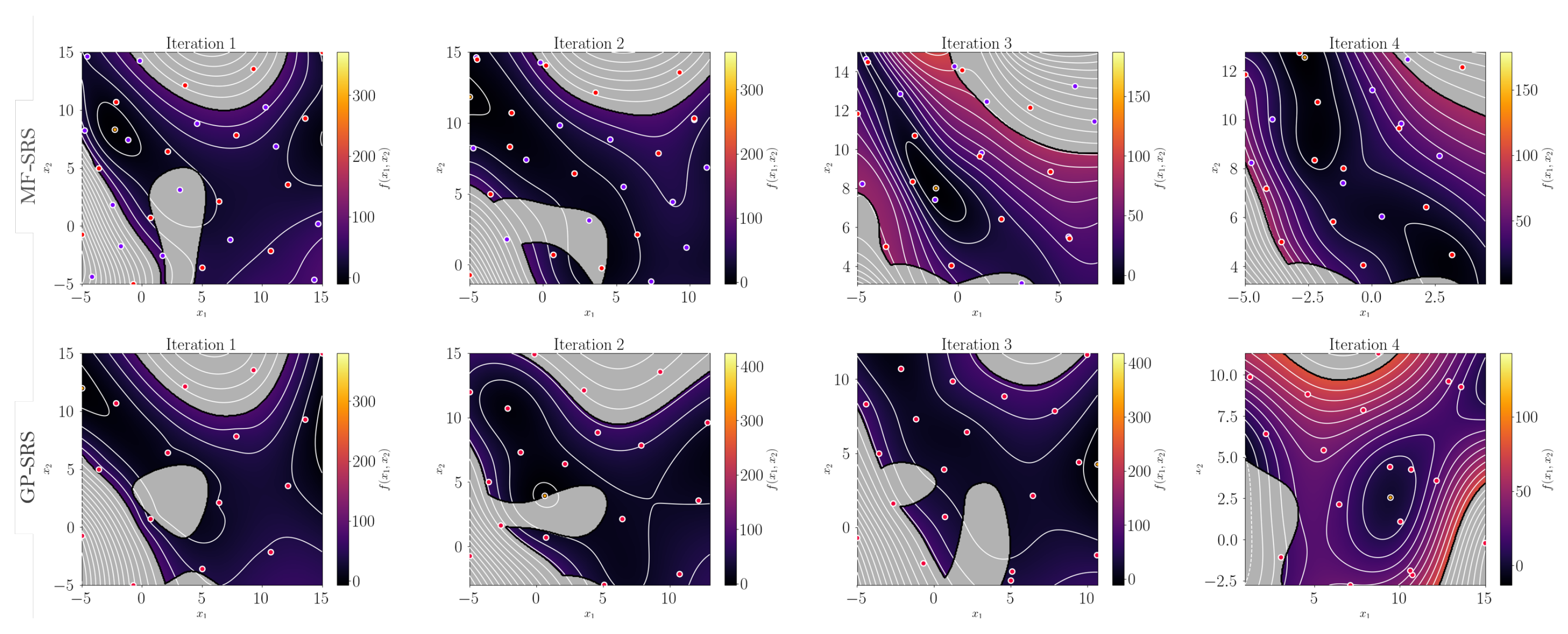
6.1. Synthetic Illustrative Problems

We begin with a visual illustration of two well-known problems in the literature of multi-fidelity functions: The Forrester function and the Sinusoidal Wave function have been presented in the works of [36,52], respectively. We break down the mathematical formula of the Forrester into its fidelities in Equations (26) and (27), while the high- and low-fidelity functions of the Sinusoidal Wave are described in Equations (28) and (29).
The multi-fidelity Forrester function is
f h i g h ( x ) = ( 6 x 2 ) 2 sin ( 12 x 4 )
f l o w ( x ) = 0.5 f h i g h ( x ) + 10 ( x 0.5 ) 5 .
The multi-fidelity Sinusoidal Wave function is
f h i g h ( x ) = ( x 2 ) · f l o w 2 ( x )
f l o w ( x ) = sin ( 8 π x ) .
The inclusion of these formulas is important to show the different types of mappings between the fidelities of these two functions. The dominance of the “linear mapping” in the Forrester function is clearly seen in the 0.5 f h i g h term, while the quadratic mapping between the fidelities of the sine wave is also recognizable. The upper part of Figure 5 shows the overall trend of these functions. The high-fidelity functions are shown in red, while the low-fidelity ones are shown in violet. The lower part of the same figure plots the correlation between the fidelity levels. It can be seen that, unlike the sine wave, the Forrester function has a predominantly linear type of correlation.
To caution readers against drawing simplistic conclusions, we would like to point out that the idea of a linear mapping between the high-fidelity and the low-fidelity representations in the Forrester function is just a simplification, commonly used for illustrative purposes in multi-fidelity contexts. This does not mean that a plot of f h i g h ( x ) over f l o w ( x ) will yield a perfectly straight line over the entire range of the function. Indeed, this would have been the case if there were no deviations induced by the bias term 10 ( x 0.5 ) , which is linear in x but not in f h i g h ( x ) .
To observe the practical implications of the theory outlined in Section 4, we approach comparing GP, AR1, and NARGP methods on these two functions. As a rule of thumb for these experiments, we always used twice as many high-fidelity observations for the low-fidelity level. Note that this number depends strongly on the problem at hand, and especially on the “cost” ratio of the fidelities. While comparing GP and multi-fidelity models may seem unfair, it serves as an insightful exercise. This comparison highlights the capability of multi-fidelity models to assimilate valuable information from alternative sources, potentially leveraging it for faster convergence.
The results for the Forrester function, based on five observations, are shown in Figure 6. Without delving into error metrics, it is evident that the multi-fidelity methods perform similarly, representing the function with greater precision compared to GP. Indeed, NARGP and AR1 show comparable performance in terms of mean and uncertainty. The most noticeable differences with GP appear at domain boundaries and within the valley of the optimum. In these regions, low-fidelity observations contribute valuable information that a conventional GP model cannot exploit.
A different scenario can be seen in Figure 7. Based on seven high-fidelity observations, the GP and AR1 methods appear to have a remarkably similar posterior distribution that deviates significantly from the true sinusoidal trend. While the subpar metamodeling of GP can be justified by the low sampling rate with respect to the period of the function, the performance of the AR1 is rather surprising. It seems to struggle to exploit the information from the low-fidelity observations. In contrast, NARGP, while not a perfect representation of the original function, seems to capture its periodic pattern and average amplitude, providing a much more accurate approximation. These results echo the key observations of Perdikaris et al. and suggest that NARGP may be a superior and more reliable option for navigating intricate relationships between fidelities.

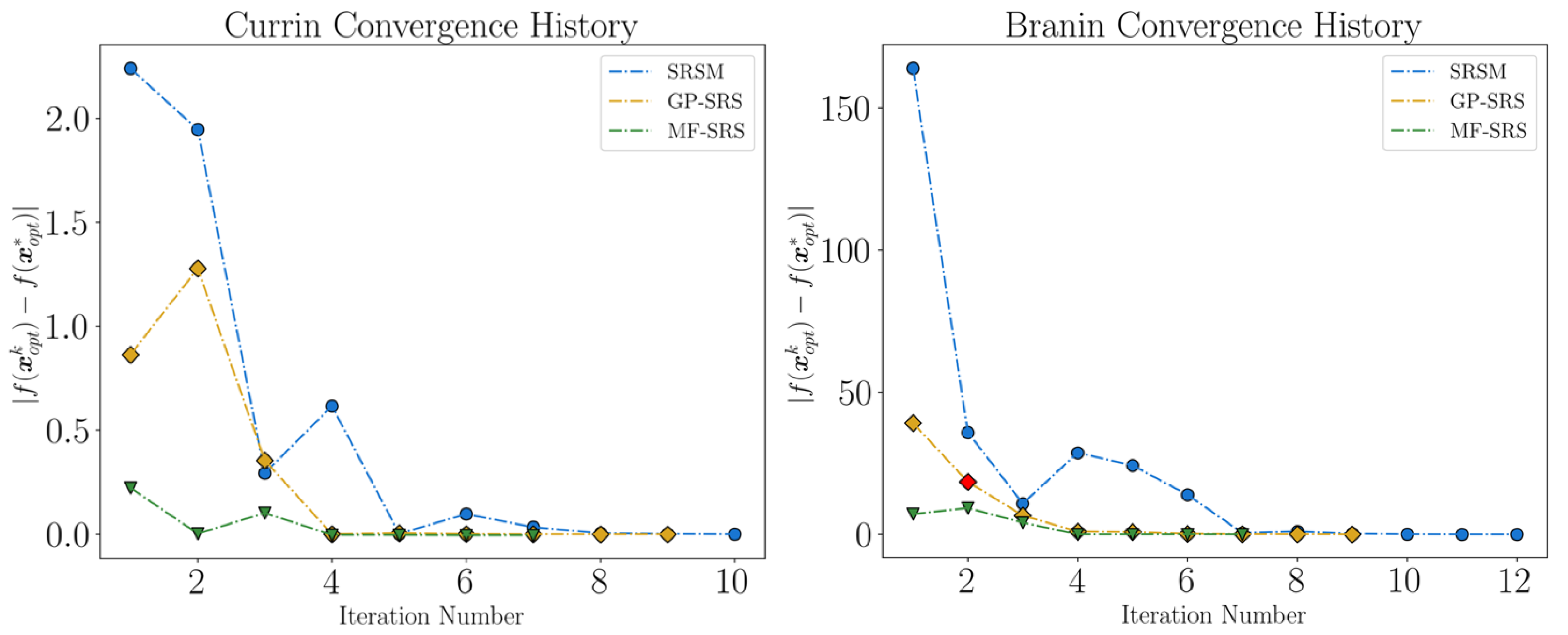
6.2. Results on Benchmark Functions

We continue our experiments with tests on benchmark functions, aiming to evaluate the convergence performance of the MF-SRS method in terms of speed and effectiveness. We aim to compare our method with its simplified variant, GP-SRS, which relies solely on GP and high-fidelity, and with the SRSM method based on PRS. Given our primary focus on crashworthiness problems, the objective remains to identify the best achievable local optimum with the least number of function evaluations. Our general expectation is to see a clear predominance of Gaussian process-based methods over polynomial regression-based approaches. We also hope to see possibly more efficient convergence of MF-SRS than GP-SRS, especially in the first few iterations, although we do not necessarily expect superior performance in the long run.
For this evaluation, we leverage the work of van Rijn and Schmitt [53], who have gathered a set of well-known benchmark functions from the literature, each with at least two levels of fidelity. The mathematical formula of those functions and further details regarding the input variables can be found in Appendix B. Specifically, we investigate:
  • The Currin function [54]: a 2D single-objective problem.
  • The Branin and Himmelblau functions [55]: a 2D double-constrained single-objective problem.
  • The Borehole function [54]: an 8D single-objective problem.
For the first problem, the goal is to either maximize or minimize the negative counterpart of the Currin function. We specify that each method starts with an equal set of high-fidelity points, 10 in this case. After each iteration, both GP-SRS and SRSM add six more high-fidelity samples, while MF-SRS introduces only four. The ratio of low-fidelity to high-fidelity samples remains constant at 2:1. For these analytical functions, which do not come with any evaluation cost, we will consistently use twice the number of low-fidelity samples compared to high-fidelity samples, similar to what is shown in [36].
The comparison between MF-SRS and GP-SRS of the first four iterations is shown in Figure 8. The first iteration highlights the value of low-fidelity samples; while GP-SRS suffers from severe overfitting complications, making it difficult to extract valuable information, MF-SRS shows a more stable progression, guiding the optimization toward the optimum despite having fewer high-fidelity samples. Both methods appear to converge quickly to the global minimum. In a second two-dimensional test, we focus on minimizing a double-constrained Branin function. We impose a constraint on the objective function itself, thereby preserving the nearly flat region where the three global minima of the function lie. In addition, we further narrow down this region through a constraint applied to the Himmelblau function, as shown by Equations (30)–(33):
min x     f b r a n i n ( x )
subject to g h i m m e l b l a u ( x ) 60 ,
g b r a n i n ( x ) 80 ,
5 x i 15 , i = 1 , 2 .
From the first four iterations shown in Figure 9, it is quite clear that the combination of the given constraints poses a significant challenge for accurate representation, especially with only 15 high-fidelity observations available. However, while the GP-SRS method bounces between opposite sides of the variable domain during the initial iteration steps, the MF-SRS method exhibits more stable behavior. It guides the RoI toward a global minimum from the first iteration, consistently avoiding the infeasible region.
We then analyze the convergence behavior of both problems and include the SRSM approach in the comparison for a more comprehensive evaluation. It is important to note that, for the SRSM method, a quadratic PRS was used. As explained in Section 3, this requires a minimum of six observations when dealing with two variables. Our expectations were indeed met. For both problems, the SRSM method is significantly the slowest to converge and consistently produces qualitatively worse results than the other methods at almost every iteration (see Figure 10). The initial investment in MF-SRS seems to pay off, as it consistently outperforms the other methods in making more accurate predictions, especially in the early steps. The lack of high-fidelity points does not seem to affect its performance, and the efficient use of all available points seems to be a key feature contributing to its effectiveness. The choice of MF-SRS over GP-SRS under these conditions would depend on the computational cost associated with different fidelity levels, as well as the potential for job submissions that utilize multiple computing resources.
As our final synthetic problem, we examine the Borehole function, an eight-dimensional problem. This function models the flow of water through a borehole drilled from the ground surface through two different aquifer layers. The flow rate of water, expressed in cubic meters per year (m 3 /year), is described by the properties of both the borehole and the aquifers. The borehole function is often used to compare different types of metamodels and to perform feature importance analysis. Since the optimum of this function is known, we aim to minimize the problem and to compare the predictions of the surface response models at the initial stage.
Considering the complexity of this problem, we initiate the process with a dataset of 80 high-fidelity samples for each method. In each subsequent iteration, we add four, six, and nine new samples for the MF-SRS, GP-SRS, and SRSM methods, respectively. It is important to note that, for the SRSM method, a linear polynomial form was employed due to the prohibitively high cost associated with such a large number of function evaluations. Indeed, this form requires d + 1 samples, which, although still quite expensive, is more manageable than the ( d + 1 ) ( d + 2 ) / 2 samples that would be required otherwise.
The initial prediction performance is depicted on the left side of Figure 11, where it is compared with the ground-truth values. The MF-SRS method demonstrates remarkable accuracy across the entire domain represented. The GP-SRS prediction is also strong, although it exhibits a larger average deviation from the ideal diagonal prediction. Notably, toward the minimum values, GP-SRS predictions are affected by a consistent bias that progressively shifts values toward the upper region of the graph. On the other hand, the SRSM method, based on PRS, exhibits the least accuracy, with a consistently higher level of uncertainty across the considered range when compared to the other two methods.
These initial prediction results are echoed in the convergence performance, illustrated on the right side of Figure 11. While none of the methods manage to reach the global optimum, MF-SRS notably outperforms the other two methods, especially in terms of efficiency, requiring 15 iterations compared to 25 and 34 (according to the convergence criterion defined in Equation (24)) for GP-SRS and SRSM, respectively. The fact that GP-SRS, despite several additional high-fidelity observations, fails to reach the same local minimum identified by the multi-fidelity method suggests that GP-SRS may have been guided toward a local minimum by a less accurate initial prediction.

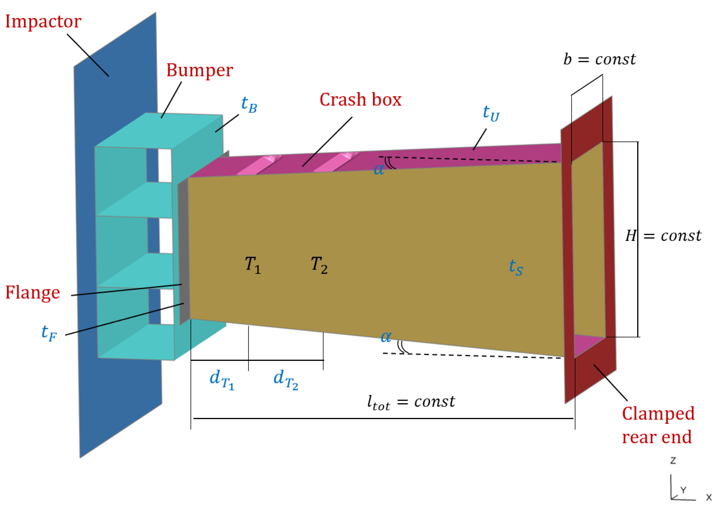
6.3. Engineering Use Case: Crash Box Design

In this section, we address the design of an aluminum crash box for an urban electric vehicle: a critical real-world engineering problem. Positioned between the bumper and longitudinal rails, this energy-absorbing device is crucial for the vehicle’s crashworthiness. It not only protects passengers and minimizes vehicle damage but can also reduce repair costs. Therefore, maximizing the energy-absorbing capability of the crash box is essential.
In this use case, we examine a structural system consisting of a bumper beam cross member, the crash box, and the crash box flange. This structure is attached to the rear end of the crash box and is subjected to compression by a rigid body, the impactor, moving at a constant velocity of 1.5 m/s. All structural components are made of AA 5083: an aluminum alloy known for its good ductility and high strength-to-weight ratio.

6.3.1. Key Performance Indicators (KPIs)

When evaluating the crashworthiness of crush boxes, a number of Key Performance Indicators (KPIs) are often examined [56,57]. These KPIs provide quantifiable metrics to assess the effectiveness of a crash box under crushing loads. An essential indicator is the total Energy Absorbed (EA). This quantifies the work performed on the structure to induce deformation due to the impact and is defined by Equation (34):
E A = 0 L c F ( x ) d x ,
where L c is the crushing length and F ( x ) denotes the resultant impact force over the displacement x. Maximizing EA is a common objective function, as long as it does not overweight the structure. To avoid this problem, it is often replaced by the Specific Energy Absorbed (SEA), which is the absorbed energy per unit mass of material:
S E A = E A m ,
where m is the sum of the mass of the crash box and the bumper beam in this case. Another important indicator is the mean crushing force, which is given by Equation (36):
F m = E A L c .
The mean crushing force is a required element for the calculation of the Undulation of Load Carrying Capacity (ULC). This indicator evaluates the stability of the structure under crushing and is given by Equation (37):
U L C = 0 L c | F ( x ) F m | d x E A .
Finally, we introduce Crushing Force Efficiency (CFE), which relates the maximum peak resistance force F m a x to the average force F m :
C F E = F m a x F m
These two critical parameters shown in Equation (38) directly affect the deceleration experienced by vehicle passengers during a collision. Ideally, an absorber will have a CFE equal to one, meaning that the crush box absorbs energy uniformly throughout the deformation process and behaves in a controlled manner under crash conditions.

6.3.2. Problem Formulation

An overview of the structural system to be analyzed is given in Figure 12. Note that there are two V-notch crush initiators (sometimes called triggers) T 1 and T 2 at the top and bottom of the crash box. These are strategically placed engineering features introduced into the crash box components of the vehicle structure to control the deformation path during a collision.
As design variables, we consider the thicknesses of the crash box ( t U and t S ), the flanges ( t F ), and the bumper cross member ( t B ). Additionally, we consider the distance from the flanges to the first trigger ( d T 1 ), the distance between the two triggers ( d T 2 ), and the angle ( α ), which symmetrically adjusts the tilt of both the top and bottom faces of the crash box with respect to the horizontal plane. The last three variables imply a change in the geometry of the crash box, classifying the problem as a mixture of size and shape optimization. A detailed description of the design variables and their respective bounds is given in Table 1.
The main objective is to maximize the SEA within certain passive safety constraints. First, we set a value for the maximum peak deformation force F m a x and a maximum value for the average deformation force F m . This is to ensure that the crash box deforms before the longitudinal members, thus ensuring a step-wise increasing deformation curve [58]. With reference to Figure 13 we set a threshold of 61.75 kN for F m a x (5% safety margin) and a threshold of 50 kN for F m .
To ensure effective energy absorption, we set a minimum threshold for the energy absorption of the bumper cross member after 35 ms, aligning with the expected timing of the first peak force due to crash box deformation. This constraint prevents excessively stiff bumper configurations that could cause premature deformation of the crash box. Additionally, we require that C F C 0.5 and U L C 0.5 . Although these constraints are typically applied to crash boxes alone, in this context, they are employed to ensure an adequate trade-off between force fluctuations and the initial peak relative to the mean force value. The complete formulation of this optimization problem is provided in Appendix C.1.

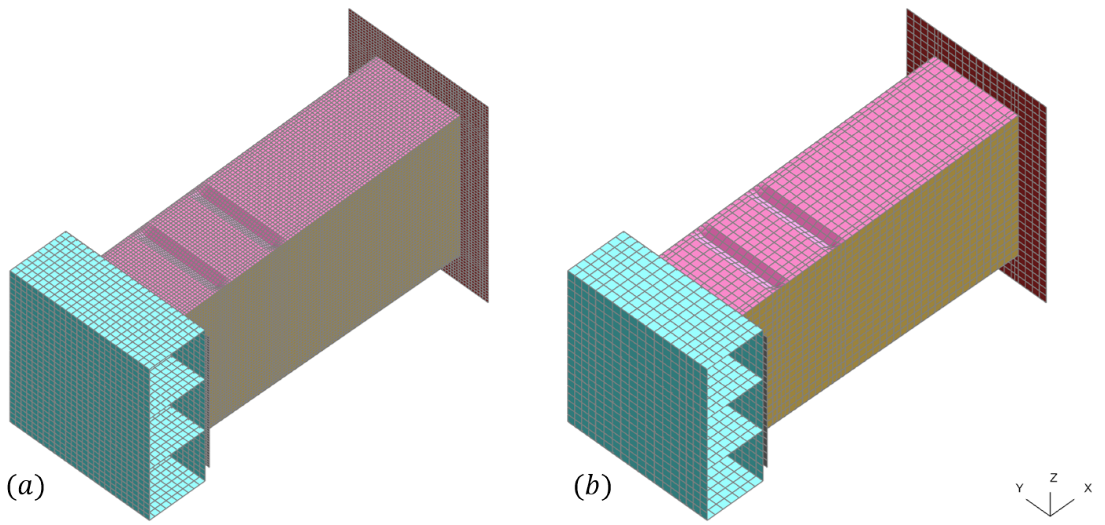
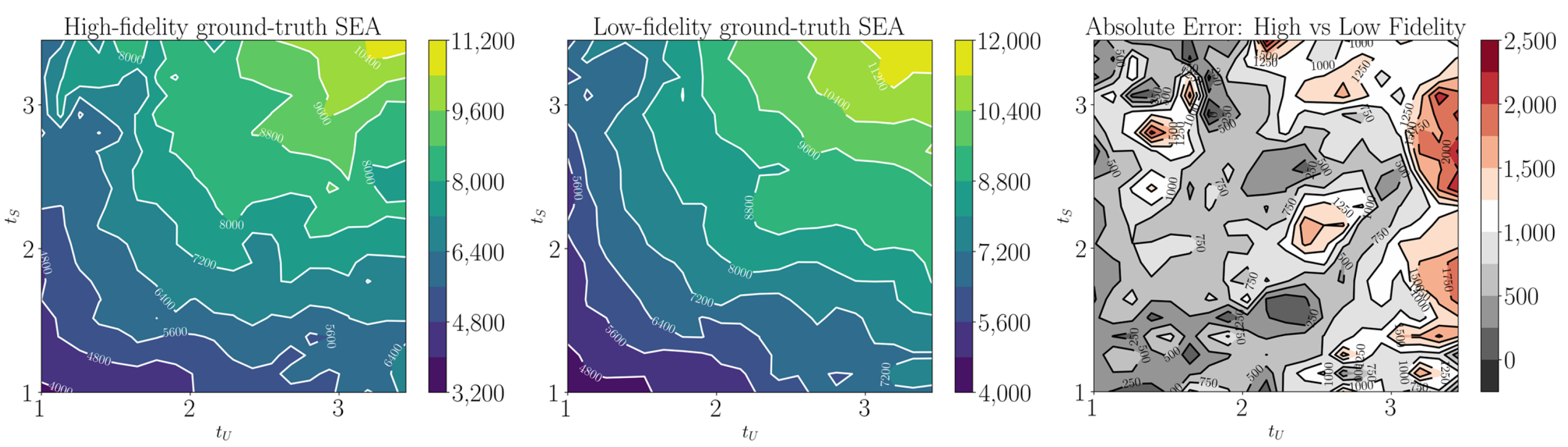
6.3.3. High- and Low-Fidelity Models

Before diving into the optimization, we need to distinguish the two fidelities for the MF-SRS method. To determine an optimal mesh size for the high-fidelity model, we performed a mesh sensitivity analysis by varying the average element size. As shown in Figure 14, reducing the mesh size below 2 mm has minimal impact on the response functions considered. However, this size reduction significantly increases the simulation time. For example, on a 2× AMD EPYC 7601 (32 cores, 2.2 GHz) per node of our HPC cluster, the time changes from 20 min to 1 h and 26 min. Based on this analysis, we chose an average mesh size of 2 mm for the high-fidelity model.
Beyond mesh size, the presence of the damage model, which defines the failure criterion for element deletion, is another significant factor that affects the duration of a simulation. Disabling this feature in our aluminum material card results in approximately a 25% reduction of simulation time for the 2 mm finite element model. In addition, increasing the mesh size to 5 mm dramatically drops the simulation time to approximately 3 min and 10 s. While this coarser finite element model is obviously less accurate and deviates from the response of the high-fidelity model, we propose its utility as a low-fidelity model. We believe that it can capture significant global information that, when integrated with high-fidelity runs, contributes significantly to the prediction of response functions. The two models are illustrated in Figure 15.
For a more thorough understanding of the use case, we carried out additional simulations to provide a broader view of the correlation between the high-fidelity and low-fidelity models. This additional analysis serves to stress the complex relationship between the two models, allowing for a more sound interpretation of the results. Detailed results and discussions from these additional simulations are provided in Appendix C.3.

6.4. Results of the Engineering Use Case

In this section, we present the results of the crash box optimization, comparing the three approaches introduced so far: SRSM, GP-SRS, and MF-SRS. For the MF-SRS approach, we use a high-fidelity DoE consisting of 60 points, with an addition of four more high-fidelity points at each iteration. Since the “cost” of low-fidelity simulations is less than one-sixth of the high-fidelity ones, we set the 2:1 ratio that has shown great results so far. In contrast, the GP-SRS approach uses a slightly larger DoE of 70 points and adds five high-fidelity points to each iteration. The SRSM method also starts with a 70-point DoE and iteratively adds eight high-fidelity points at each iteration based on the linear polynomial criterion.
To achieve faster and more robust convergence, at each iteration, we record the best feasible value using the criterion given in Formula (24) based on n A R F T = 4 . If this value does not improve, we retain the best feasible value achieved in prior iterations. If all designs at a specific iteration fail to meet the constraints, we mark the point in red. From the results shown in Figure 16, the performance of MF-SRS stands out. It is clearly the most effective approach, achieving a 13.1% and a 14.1% SEA improvement over GP-SRS and SRSM, respectively. Alongside the improved optimum, the fast convergence and the ability to accurately predict the feasibility limits of the domain are remarkable. This is particularly evident in the result of the first iteration where, despite the deficit of 10 high-fidelity points, MF-SRS still manages to identify an optimum that outperforms the other approaches.
The performance of GP-SRS is solid, although with a slower progression than expected. We believe that with more relaxed convergence criteria, it may eventually surpass the maximum obtained by MF-SRS, albeit at a significantly higher computational cost.
Conversely, SRSM appears to be the least robust approach. Despite the rapid improvement in the fourth iteration, the best-reported point often does not match with the verification point, which is a discrepancy that is curious considering the predictive potential offered by the eight new high-fidelity samples added at each iteration. From a computational point of view, SRSM seems to be the most “expensive” and, in terms of prediction, the most unreliable of the methods investigated. Further details of the optimal designs of response values and input variables are provided in Table 2 and Appendix C.4, respectively.
The iteration by iteration evolution of the MF-SRS method is shown in the parallel coordinates plot in Figure 17. The light gray lines represent designs that violate the constraints and are, therefore, unfeasible, while the blue lines denote feasible designs. It is clear that the density of the darker lines increases around the optimal design, which is shown in orange. This provides further evidence of the robust convergence of the MF-SRS method.
The deformation force versus impactor displacement pattern is shown in Figure 18. Although very similar in the first peak force (about 45 mm), the higher energy absorption is in the crash box folding behavior with a higher average force value. As for the bumper design, the MF-SRS method has probably room for improvement given the lower energy absorption.

6.5. Parallel Job Submission on an HPC

While we have primarily assessed convergence curves on an iteration-wise basis, careful observers may rightly argue that this comparison does not fully account for efficiency. Specifically, the MF-SRS method incurs an extra cost due to low-fidelity simulations, different methods adding a different number of high-fidelity samples at each iteration, and the MF-SRS starting with a DoE with 10 fewer high-fidelity samples. Taking these factors into account, in this section, we delve into how the curves in Figure 16 adjust when viewed in terms of cumulative computational time, with a particular focus on the HPC logic implications.
Before presenting the results, we outline some assumptions:
  • We use a cluster of N n o d e s with 2 × 32 cores each (AMD EPYC 7601 processors);
  • Only one job is submitted on each node at a time. Parallel job submissions across different nodes are allowed, but splitting a single node among multiple jobs is not;
  • We use a greedy job scheduler that ideally distributes jobs across nodes once the optimization problem is defined. We assume that the availability of nodes at any given time does not affect the formulation of the optimization problem;
  • We assume that the computational cost of low-fidelity jobs is equivalent to a unit cost. Therefore, given the cost ratio, we know that a high-fidelity job has a cost of 6.25 units for this particular problem.
Bear in mind that the job scheduler prioritizes parallelization of high-fidelity jobs across available nodes. It allocates low-fidelity jobs only after all the more demanding high-fidelity simulations are completed.
Assuming the availability of five, seven, and eight nodes, the results are displayed in Figure 19, from left to right, respectively. The top row illustrates the prioritization of multi-fidelity DoE jobs according to the described scheduling logic. The bottom row presents the full convergence curve, plotted against the cumulative computational cost. The chosen node configurations ideally suit each of the three methods investigated. In fact, with regard to the MF-SRS method, five nodes in parallel guarantee an exact division (without a remainder) both for the number of high-fidelity samples of the DoE and for the number of samples added iteratively. Similarly, seven and eight nodes are scenarios that favor the GP-SRS and SRSM methods, respectively. We observe that, due to the additional cost of the additional simulations with the coarse mesh, the first iteration of the multi-fidelity approach is no longer vertically aligned with the other two. However, due to its cost-ratio advantage and limited use of high-fidelity points, the MF-SRS method consistently emerges as the most efficient approach, regardless of the number of nodes available. Any unused nodes can be eventually assigned to handle batches of low-fidelity jobs, efficiently utilizing computational resources while waiting for more resource-intensive simulations to complete. These results emphasize how parallel job scheduling can be leveraged to make the MF-SRS method even more efficient and competitive.

7. Conclusions

In this paper, we introduced the MF-SRS method, a novel optimization approach that leverages Gaussian processes to better handle the inherent complexity of crashworthiness problems.
While the traditional SRSM is effective in some aspects, it has been found to have significant limitations, particularly in the prohibitive use of costly function evaluations and the shortcomings associated with the PSR method. The proposed MF-SRS method addresses these challenges by employing a multi-fidelity approach that captures in-depth information from both high-fidelity and low-fidelity models, wisely reuses information from previous iterations, and queries new data at unexplored locations via adaptive infill seed criteria. This combination results in a more robust and versatile framework compared to SRSM.
Our experiments, ranging from benchmark functions to a real-world crashworthiness application, yielded promising results. MF-SRS consistently demonstrated improved performance over both SRSM and GP-SRS, despite the initial additional cost of low-fidelity evaluations. Specifically, it achieved a remarkable 14.1% improvement in the optimal value of specific energy absorption over SRSM, underscoring the stability and precision of the optimization process. This efficiency is even more pronounced when considering its ability to achieve optimal values with less computational burden. The extent of such burden depends on several factors, including available computational power and parallel job logic on an HPC. Moreover, in a scenario characterized by a low-fidelity model with a coarse mesh and no element erosion, MF-SRS successfully detected intricate relationships between different fidelities, reinforcing its effectiveness and efficiency in various application contexts.
In our future research, we plan to primarily investigate the optimal ratio of high- and low-fidelity points per iteration and within the initial DoE, with the aim of adaptively adjusting these numbers based on the given problem. While NARGP stands out as a promising multi-fidelity approach, this rapidly evolving field introduces exciting alternatives at a rapid pace. Of particular interest are Multi-Fidelity Bayesian Neural Network approaches, which offer the potential to address uncertainties in sampling and to capture intricate correlations between fidelities thanks to the Neural Network framework. Finally, tailoring specific covariance functions relevant to certain iterations within the GP-SRS method offers another intriguing avenue of exploration.

Author Contributions

Conceptualization, P.L. and R.S.; methodology, P.L.; software, P.L.; validation, P.L.; formal analysis, P.L., R.S. and T.S.; investigation, P.L.; resources, P.L. and R.S.; data curation, P.L.; writing—original draft preparation, P.L. and R.S.; writing—review and editing, R.S. and T.S.; visualization, P.L.; supervision, R.S. and T.S.; project administration, R.S.; funding acquisition, R.S. All authors have read and agreed to the published version of the manuscript.

Funding

This research received no external funding.

Data Availability Statement

The data used to support the findings of this study are available from the corresponding author upon request.

Acknowledgments

We would like to express our sincere gratitude to Andrew Harrison, Thomas Grünheid-Ott, and Daniel Grealy for their valuable contributions.

Conflicts of Interest

The authors declare no conflict of interest.

Abbreviations

The following abbreviations are used in this manuscript:
AR1Auto-Regressive Order 1
GPGaussian Process
GP-SRSGaussian Process Successive Response Surface
MF-SRSMulti-Fidelity Successive Response Surface
NARGPNon-Linear Auto-Regressive Gaussian Process
PRSPolynomial Response Surface
SRSMSuccessive Response Surface Method

Appendix A

The main idea behind the mc-inter-proj-th (MIPT) [38] method is discarding candidates that lie too close to each other based on the projected distance based on a threshold value. The remaining points are then ranked on their intersite distance. Therefore, this Monte Carlo method looks as follows:
M I P ( P , p ) = 0 if min p i P p i p < d min p i P p i p 2 if min p i P p i p d ,
where the threshold d m i n is defined by a tolerance parameter α , which has a domain of [ 0 , 1 ] :
d m i n = 2 α n .
The tolerance parameter α defines the balance between the space-filling and non-collapsing properties. Low values of α lead to a reduction in the projected distance constraint. Therefore, fewer candidates are discarded. On the other hand, high values of α result in a strict constraint to be satisfied. This reduces the chance of finding a valid candidate [6].

Appendix B

The Currin function is given by
f h ( x ) = 1 exp ( 1 2 x 2 ) 2300 x 1 3 + 1900 x 1 2 + 2092 x 1 + 60 100 x 1 3 + 500 x 1 2 + 4 x 1 + 20
f l ( x ) = ( f h ( x 1 + 0.05 , x 2 + 0.05 ) + f h ( x 1 + 0.05 , x 2 0.05 ) + f h ( x 1 0.05 , x 2 + 0.05 ) + f h ( x 1 0.05 , x 2 0.05 ) ) / 4
x o p t = { ( 13 60 , 0 ) } .
The Branin function is given by
f b ( x ) = x 2 ( 5.1 x 1 2 4 π 2 ) + 5 x 1 π 6 2 + 10 cos ( x 1 ) ( 1 1 8 π + 10
f h ( x ) = f b ( x 1 , x 2 ) 22.5 x 2
f l ( x ) = f b ( 0 . 7 1 , 0.7 x 2 ) 15.75 x 2 + 20 ( 0.9 + x 1 ) 2 50
x o p t = { ( π , 12.275 ) , ( π , 2.275 ) , ( 9.42478 , 2.475 ) } .
The Himmelblau function is given by
f h ( x ) = ( x 1 2 + x 2 11 ) 2 + ( x 2 2 + x 1 7 ) 2
f l ( x ) = f h ( 0.5 x 1 , 0.8 x 2 ) + x 2 3 ( x 1 + 1 ) 2
x o p t = { ( 3.0 , 2.0 ) , ( 2.805118 , 3.131312 ) , ( 3.779310 , 3.283186 ) , ( 3.584428 , 1.848126 ) } .
The Borehole function is given by
f ( x , A , B ) = A · T u · ( H u H l ) log r r w B + 2 L · T u log r r w · r w 2 · K w + T u T l
f h i g h ( x ) = f ( x , 2 π , 1 )
f l o w ( x ) = f ( x , 5 , 1.5 )
x o p t = { ( 0.05 , 50000.0 , 63070.0 , 990.0 , 63.1 , 820.0 , 1680.0 , 9855.0 ) } ,
where
T u = radial flow of the upper aquifer ( m 2 / year ) T l = radial flow of the lower aquifer ( m 2 / year ) H u = potentiometric head of the upper aquifer ( m ) H l = potentiometric head of the lower aquifer ( m ) L = length of the borehole ( m ) K w = hydraulic conductivity of the borehole ( m / year ) r = radius of influence ( m ) r w = radius of the borehole ( m )

Appendix C

Appendix C.1

The crash box optimization problem, from a mathematical point of view, is defined as follows:
max x S E A ( x )
  subject to F m a x ( x ) 61.75 k N ,
F m ( x ) 50.0 k N ,
E A B ( x , t = 35 ) 100 J ,
C F E ( x ) 0.5 ,
U L C ( x ) 0.5 ,
1.0 t U 3.5 ,
1.0 t S 3.5 ,
1.0 t B 3.5 ,
1.0 t F 4.0 ,
  20.0 d T 1 70.0 ,
30.0 d T 2 100.0 ,
1.0 α 4.5 .

Appendix C.2

Table A1 provides the specifications for both high-fidelity and low-fidelity FE models that are to be simulated using the LS-DYNA explicit solver (single precision, version 11.1). The material model refers to the crash box only, while the impactor is considered as a rigid body with its own material formulation. The contact type describes the primary interaction between the crash box and the rigid plate.
Table A1. Details of high-fidelity and low-fidelity FE Models.
ParameterHigh-Fidelity ModelLow-Fidelity Model
Number of Nodes23,8266082
Number of Elements23,5485940
Material Model* MAT_024
Element TypeShell Belytschko-Tsay
Contact TypeAUTOMATIC_SURFACE_TO_SURFACE
ErosionActiveInactive
* MAT_PIECEWISE_LINEAR_PLASTICITY.

Appendix C.3

In Figure A1, we illustrate the SEA correlation between the two fidelities with respect to the variables t U and t S , holding all other variables constant. This correlation is visualized by a 20 × 20 grid showing the ground-truth values derived from numerical simulations.
Figure A1. Contour plots representing SEA values across a 20 × 20 grid. From left to right: high-fidelity ground-truth values, low-fidelity ground-truth values, and the absolute error between the two fidelity levels.
Applsci 13 11452 g0a1
Although the low-fidelity model roughly mirrors the pattern of its high-fidelity counterpart, it is noticeable that the relationship between the two is not uniform across the 2D domain. In certain local regions, the absolute error exceeds 2000 J/kg, indicating a complex, non-linear relationship that requires careful management in the learning process. A similar relationship can be observed in F max , as shown in Figure A2.
Figure A2. Contour plots representing F m a x values across a 20 × 20 grid. From left to right: high-fidelity ground-truth values, low-fidelity ground-truth values, and the absolute error between the two fidelity levels.
Applsci 13 11452 g0a2

Appendix C.4

Table A2. Summary of the optimal design variables of each method.
Method t U (mm) t S (mm) t B (mm) t F (mm) d T 1 (mm) d T 2 (mm) α (deg)
SRSM2.12.61.01.030.140.01.0
GP-SRS2.32.51.21.733.231.12.8
MF-SRS2.42.71.01.536.230.02.7

References

  1. O’Neill, B. Preventing passenger vehicle occupant injuries by vehicle design—A historical perspective from IIHS. Traffic Inj. Prev. 2009, 10, 113–126. [Google Scholar] [CrossRef]
  2. Sacks, J.; Welch, W.J.; Mitchell, T.J.; Wynn, H.P. Design and Analysis of Computer Experiments. Stat. Sci. 1989, 4, 409–423. [Google Scholar] [CrossRef]
  3. Bartz-Beielstein, T.; Zaefferer, M. Model-based methods for continuous and discrete global optimization. Appl. Soft Comput. 2017, 55, 154–167. [Google Scholar] [CrossRef]
  4. Khatouri, H.; Benamara, T.; Breitkopf, P.; Demange, J. Metamodeling techniques for CPU-intensive simulation-based design optimization: A survey. Adv. Model. Simul. Eng. Sci. 2022, 9, 1. [Google Scholar] [CrossRef]
  5. Kleijnen, J.P.C. A Comment on Blanning’s “Metamodel for Sensitivity Analysis: The Regression Metamodel in Simulation”. Interfaces 1975, 5, 21–23. [Google Scholar] [CrossRef]
  6. Lualdi, P.; Sturm, R.; Siefkes, T. Exploration-oriented sampling strategies for global surrogate modeling: A comparison between one-stage and adaptive methods. J. Comput. Sci. 2022, 60, 101603. [Google Scholar] [CrossRef]
  7. Rasmussen, C.E.; Williams, C.K.I. Gaussian Processes for Machine Learning; Adaptive Computation and Machine Learning; MIT: Cambridge, MA, USA; London, UK, 2006. [Google Scholar]
  8. Myers, R.H.; Montgomery, D.C.; Anderson-Cook, C.M. Response Surface Methodology: Process and Product Optimization Using Designed Experiments, 4th ed.; Wiley Series in Probability and Statistics; Wiley: Hoboken, NJ, USA, 2016. [Google Scholar]
  9. Montgomery, D.C. Design and Analysis of Experiments, 10th ed.; John Wiley & Sons, Inc.: Hoboken, NJ, USA, 2021. [Google Scholar]
  10. Gunn, S.R. Support Vector Machines for Classification and Regression; University of Southampton Institutional Repository: Southampton, UK, 1998. [Google Scholar]
  11. Wang, T.; Li, M.; Qin, D.; Chen, J.; Wu, H. Crashworthiness Analysis and Multi-Objective Optimization for Concave I-Shaped Honeycomb Structure. Appl. Sci. 2022, 12, 420. [Google Scholar] [CrossRef]
  12. Pawlus, W.; Robbersmyr, K.G.; Karimi, H.R. Performance Evaluation of Feed Forward Neural Networks for Modeling a Vehicle to Pole Central Collision; World Scientific and Engineering Academy and Society (WSEAS): Stevens Point, WI, USA, 2011. [Google Scholar]
  13. Omar, T.; Eskandarian, A.; Bedewi, N. Vehicle crash modelling using recurrent neural networks. Math. Comput. Model. 1998, 28, 31–42. [Google Scholar] [CrossRef]
  14. Fang, J.; Sun, G.; Qiu, N.; Kim, N.H.; Li, Q. On design optimization for structural crashworthiness and its state of the art. Struct. Multidiscip. Optim. 2017, 55, 1091–1119. [Google Scholar] [CrossRef]
  15. Duddeck, F. Multidisciplinary optimization of car bodies. Struct. Multidiscip. Optim. 2008, 35, 375–389. [Google Scholar] [CrossRef]
  16. Holland, J.H. Adaptation in Natural and Artificial Systems: An Introductory Analysis with Applications to Biology, Control, and Artificial Intelligence, 1st ed.; The MIT Press: Cambridge, UK, 1992. [Google Scholar]
  17. Bäck, T. Evolutionary Algorithms in Theory and Practice: Evolution Strategies, Evolutionary Programming, Genetic Algorithms; Thomas Bäck; Oxford University Press: Oxford, UK; New York, NY, USA, 1996. [Google Scholar]
  18. Slowik, A.; Kwasnicka, H. Evolutionary algorithms and their applications to engineering problems. Neural Comput. Appl. 2020, 32, 12363–12379. [Google Scholar] [CrossRef]
  19. Kirkpatrick, S.; Gelatt, C.D.; Vecchi, M.P. Optimization by simulated annealing. Science 1983, 220, 671–680. [Google Scholar] [CrossRef]
  20. Kurtaran, H.; Eskandarian, A.; Marzougui, D.; Bedewi, N.E. Crashworthiness design optimization using successive response surface approximations. Comput. Mech. 2002, 29, 409–421. [Google Scholar] [CrossRef]
  21. Stander, N.; Craig, K.J. On the robustness of a simple domain reduction scheme for simulation–based optimization. Eng. Comput. 2002, 19, 431–450. [Google Scholar] [CrossRef]
  22. Liu, S.T.; Tong, Z.Q.; Tang, Z.L.; Zhang, Z.H. Design optimization of the S-frame to improve crashworthiness. Acta Mech. Sin. 2014, 30, 589–599. [Google Scholar] [CrossRef]
  23. Naceur, H.; Guo, Y.Q.; Ben-Elechi, S. Response surface methodology for design of sheet forming parameters to control springback effects. Comput. Struct. 2006, 84, 1651–1663. [Google Scholar] [CrossRef]
  24. Acar, E.; Yilmaz, B.; Güler, M.A.; Altin, M. Multi-fidelity crashworthiness optimization of a bus bumper system under frontal impact. J. Braz. Soc. Mech. Sci. Eng. 2020, 42, 493. [Google Scholar] [CrossRef]
  25. Lönn, D.; Bergman, G.; Nilsson, L.; Simonsson, K. Experimental and finite element robustness studies of a bumper system subjected to an offset impact loading. Int. J. Crashworthiness 2011, 16, 155–168. [Google Scholar] [CrossRef]
  26. Aspenberg, D.; Jergeus, J.; Nilsson, L. Robust optimization of front members in a full frontal car impact. Eng. Optim. 2013, 45, 245–264. [Google Scholar] [CrossRef]
  27. Nilsson, L.; Redhe, M. (Eds.) An Investigation of Structural Optimization in Crashworthiness Design Using a Stochastic Approach; Livermore Software Corporation: Dearborn, MI, USA, 2004. [Google Scholar]
  28. Redhe, M.; Giger, M.; Nilsson, L. An investigation of structural optimization in crashworthiness design using a stochastic approach. Struct. Multidiscip. Optim. 2004, 27, 446–459. [Google Scholar] [CrossRef]
  29. Stander, N.; Reichert, R.; Frank, T. Optimization of nonlinear dynamical problems using successive linear approximations. In Proceedings of the 8th Symposium on Multidisciplinary Analysis and Optimization, Long Beach, CA, USA, 6 September 2000. [Google Scholar] [CrossRef]
  30. Kennedy, M.C.; O’Hagan, A. Predicting the Output from a Complex Computer Code When Fast Approximations Are Available. Biometrika 2000, 87, 1–13. [Google Scholar] [CrossRef]
  31. Le Gratiet, L.; Garnier, J. Recursive co-kriging model for design of computer experiments with multiple levels of fidelity. Int. J. Uncertain. Quantif. 2014, 4, 365–386. [Google Scholar] [CrossRef]
  32. Duvenaud, D. Automatic Model Construction with Gaussian Processes. Ph.D. Thesis, Apollo—University of Cambridge Repository, Cambridge, UK, 2014. [Google Scholar] [CrossRef]
  33. Hagan, A.O. A Markov Property for Covariance Structures; University of Nottingham: Nottingham, UK, 1998. [Google Scholar]
  34. Forrester, A.I.J.; Sóbester, A.; Keane, A.J. Engineering Design via Surrogate Modelling: A Practical Guide; J. Wiley: Chichester West Sussex, UK; Hoboken, NJ, USA, 2008. [Google Scholar]
  35. Perdikaris, P.; Karniadakis, G.E. Model inversion via multi-fidelity Bayesian optimization: A new paradigm for parameter estimation in haemodynamics, and beyond. J. R. Soc. Interface 2016, 13. [Google Scholar] [CrossRef]
  36. Perdikaris, P.; Raissi, M.; Damianou, A.; Lawrence, N.D.; Karniadakis, G.E. Nonlinear information fusion algorithms for data-efficient multi-fidelity modelling. Proc. R. Soc. Math. Phys. Eng. Sci. 2017, 473, 20160751. [Google Scholar] [CrossRef]
  37. Van Dam, E.R.; Husslage, B.; den Hertog, D.; Melissen, H. Maximin Latin Hypercube Designs in Two Dimensions. Oper. Res. 2007, 55, 158–169. [Google Scholar] [CrossRef]
  38. Crombecq, K.; Laermans, E.; Dhaene, T. Efficient space-filling and non-collapsing sequential design strategies for simulation-based modeling. Eur. J. Oper. Res. 2011, 214, 683–696. [Google Scholar] [CrossRef]
  39. Van Dam, E.; den Hertog, D.; Husslage, B.; Rennen, G. Space-Filling Designs. 2015. Available online: https://www.spacefillingdesigns.nl/ (accessed on 15 July 2023).
  40. Viana, F.A.C.; Venter, G.; Balabanov, V. An algorithm for fast optimal Latin hypercube design of experiments. Int. J. Numer. Methods Eng. 2010, 82, 135–156. [Google Scholar] [CrossRef]
  41. Hao, P.; Feng, S.; Li, Y.; Wang, B.; Chen, H. Adaptive infill sampling criterion for multi-fidelity gradient-enhanced kriging model. Struct. Multidiscip. Optim. 2020, 62, 353–373. [Google Scholar] [CrossRef]
  42. Loeppky, J.L.; Sacks, J.; Welch, W.J. Choosing the Sample Size of a Computer Experiment: A Practical Guide. Technometrics 2009, 51, 366–376. [Google Scholar] [CrossRef]
  43. Nguyen, V.; Rana, S.; Gupta, S.K.; Li, C.; Venkatesh, S. Budgeted Batch Bayesian Optimization. In Proceedings of the 2016 IEEE 16th International Conference on Data Mining (ICDM), Barcelona, Spain, 12–15 December 2016; pp. 1107–1112. [Google Scholar] [CrossRef]
  44. Gao, B.; Ren, Y.; Jiang, H.; Xiang, J. Sensitivity analysis-based variable screening and reliability optimisation for composite fuselage frame crashworthiness design. Int. J. Crashworthiness 2019, 24, 380–388. [Google Scholar] [CrossRef]
  45. Fiore, A.; Marano, G.C.; Greco, R.; Mastromarino, E. Structural optimization of hollow-section steel trusses by differential evolution algorithm. Int. J. Steel Struct. 2016, 16, 411–423. [Google Scholar] [CrossRef]
  46. Loja, M.; Mota Soares, C.M.; Barbosa, J.I. Optimization of magneto-electro-elastic composite structures using differential evolution. Compos. Struct. 2014, 107, 276–287. [Google Scholar] [CrossRef]
  47. Storn, R. On the usage of differential evolution for function optimization. In Proceedings of the 1996 Biennial conference of the North American Fuzzy Information Processing Society, Berkeley, CA, USA, 19–22 June 1996; Smith, M.H.E., Ed.; IEEE: New York, NY, USA, 1996; pp. 519–523. [Google Scholar] [CrossRef]
  48. Storn, R.; Price, K. Differential Evolution—A Simple and Efficient Heuristic for global Optimization over Continuous Spaces. J. Glob. Optim. 1997, 11, 341–359. [Google Scholar] [CrossRef]
  49. Hansen, N.; Auger, A.; Ros, R.; Mersmann, O.; Tušar, T.; Brockhoff, D. COCO: A platform for comparing continuous optimizers in a black-box setting. Optim. Methods Softw. 2021, 36, 114–144. [Google Scholar] [CrossRef]
  50. Conn, A.R.; Gould, N.I.M.; Toint, P.L. Trust-Region Methods; MPS-SIAM Series on Optimization; SIAM: Philadelphia, PA, USA, 2000. [Google Scholar] [CrossRef]
  51. Querin, O.M.; Victoria, M.; Alonso, C.; Ansola, R.; Martí, P. Chapter 3—Discrete Method of Structural Optimization. In Topology Design Methods for Structural Optimization [Electronic Resource]; Querin, O.M., Ed.; Academic Press: London, UK, 2017; pp. 27–46. [Google Scholar] [CrossRef]
  52. Forrester, A.I.; Sóbester, A.; Keane, A.J. Multi-fidelity optimization via surrogate modelling. Proc. R. Soc. Math. Phys. Eng. Sci. 2007, 463, 3251–3269. [Google Scholar] [CrossRef]
  53. Van Rijn, S.; Schmitt, S. MF2: A Collection of Multi-Fidelity Benchmark Functions in Python. J. Open Source Softw. 2020, 5, 2049. [Google Scholar] [CrossRef]
  54. Xiong, S.; Qian, P.Z.G.; Wu, C.F.J. Sequential Design and Analysis of High-Accuracy and Low-Accuracy Computer Codes. Technometrics 2013, 55, 37–46. [Google Scholar] [CrossRef]
  55. Dong, H.; Song, B.; Wang, P.; Huang, S. Multi-fidelity information fusion based on prediction of kriging. Struct. Multidiscip. Optim. 2015, 51, 1267–1280. [Google Scholar] [CrossRef]
  56. Mortazavi Moghaddam, A.; Kheradpisheh, A.; Asgari, M. A basic design for automotive crash boxes using an efficient corrugated conical tube. Proc. Inst. Mech. Eng. Part J. Automob. Eng. 2021, 235, 1835–1848. [Google Scholar] [CrossRef]
  57. Xiang, Y.; Wang, M.; Yu, T.; Yang, L. Key Performance Indicators of Tubes and Foam-Filled Tubes Used as Energy Absorbers. Int. J. Appl. Mech. 2015, 07, 1550060. [Google Scholar] [CrossRef]
  58. Kröger, M. Methodische Auslegung und Erprobung von Fahrzeug-Crashstrukturen. Ph.D. Thesis, Hannover Universität, Hannover, Germany, 2002. [Google Scholar] [CrossRef]
Figure 1. Sequential update of the Region of Interest: (a) pure panning, (b) pure zooming, and (c) a pan-and-zoom combination.
Applsci 13 11452 g001
Figure 2. Overview of the MF-SRS framework.
Applsci 13 11452 g002
Figure 3. From left to right, sampling in order of decreasing fidelity: (a) OLHD with 10 samples ( D s ), (b) MIPT adds 20 D s 1 samples, and (c) MIPT adds 80 D s 2 samples.
Applsci 13 11452 g003
Figure 4. Progressing from left to right, the figures depict the evolution of the RoI and the subsequent addition of samples over three iterations. High-fidelity samples are represented in red, low-fidelity samples in purple, and samples from prior iterations that fall outside the RoI are shown in gray.
Applsci 13 11452 g004
Figure 5. The first row shows the ground-truth values of the Forrester (first column) and Sinusoidal Wave (second column). The bottom row illustrates the respective mapping between the fidelities.
Applsci 13 11452 g005
Figure 6. From left to right: GP, AR1, and NARGP reconstructions of the Forrester function. All use 5 high-fidelity observations; multi-fidelity methods also use 10 low-fidelity observations.
Applsci 13 11452 g006
Figure 7. From left to right: GP, AR1, and NARGP reconstructions of the Sinusoidal Wave function. All use 7 high-fidelity observations; multi-fidelity methods also use 14 low-fidelity observations.
Applsci 13 11452 g007
Figure 8. First four iterations for the Currin function: MF-SRS (top row) and GP-SRS (bottom row) are shown. Red dots represent high-fidelity observations; purple dots represent low-fidelity ones.
Applsci 13 11452 g008
Figure 9. First four iterations for the constrained Branin function: MF-SRS (top row) and GP-SRS (bottom row) are shown. Red dots represent high-fidelity observations, purple dots represent low-fidelity observations, and gray areas represent unfeasible regions.
Applsci 13 11452 g009
Figure 10. Convergence history of the SRSM, GP-SRS, and MF-SRS methods for the Currin function (left) and the constrained Branin function (right).
Applsci 13 11452 g010
Figure 11. Ground-truth vs. prediction plot (left) and convergence history (right) of the SRSM, GP-SRS, and MF-SRS methods for the Borehole function.
Applsci 13 11452 g011
Figure 12. Overview of the FEA model components: impactor, crash box, and bumper beam. The design variables of the optimization problem are highlighted in blue.
Applsci 13 11452 g012
Figure 13. Example of a step-wise increasing force curve with the smallest possible differences in the force levels of the individual components. Figure inspired by [58].
Applsci 13 11452 g013
Figure 14. Mesh sensitivity analysis to assess the impact of the element size on the response functions.
Applsci 13 11452 g014
Figure 15. High-fidelity model: 23,548 shell elements with element erosion (a) and low-fidelity model: 5940 shell elements without element erosion (b). Further comprehensive details about these models are provided in Appendix C.2.
Applsci 13 11452 g015
Figure 16. Convergence history of the SRSM, GP-SRS, and MF-SRS methods for the crash box design.
Applsci 13 11452 g016
Figure 17. Parallel coordinates plot of the MF-SRS method; unfeasible designs are highlighted in gray, feasible designs in blue, and the optimal design in orange.
Applsci 13 11452 g017
Figure 18. Force vs. displacement plots of the optimal designs for the SRSM, GP-SRS, and MF-SRS approaches.
Applsci 13 11452 g018
Figure 19. The job schedule of the multi-fidelity DoE (top row) and the convergence curves over the cumulative cost (bottom row) in the case of 5, 7, and 8 nodes available on the HPC.
Applsci 13 11452 g019
Table 1. Summary of design variables.
Variable DesignLabelUnitLower BoundUpper Bound
Upper crash box thickness t U (mm)1.03.5
Side crash box thickness t S (mm)1.03.5
Bumper cross member thickness t B (mm)1.03.0
Flange thickness t F (mm)1.04.0
Flange to T 1 distance d T 1 (mm)20.070.0
T 1 to T 2 distance d T 2 (mm)30.0100.0
Angle to horizontal plane α ( d e g ) 1.03.5
Table 2. Summary of the response functions of the optimal designs of each method. The best achievable SEA value among the three methods is highlighted in bold.
Method n i t e r S E A (J/kg) F m a x (kN) F m (kN) E A B (J) C F E U L C
SRSM198159.851.926.9271.90.520.48
GP-SRS178233.259.028.5260.80.510.48
MF-SRS159313.561.531.9244.20.510.49
Disclaimer/Publisher’s Note: The statements, opinions and data contained in all publications are solely those of the individual author(s) and contributor(s) and not of MDPI and/or the editor(s). MDPI and/or the editor(s) disclaim responsibility for any injury to people or property resulting from any ideas, methods, instructions or products referred to in the content.

