Pipelined Stochastic Gradient Descent with Taylor Expansion

Abstract

Stochastic gradient descent (SGD) is an optimization method typically used in deep learning to train deep neural network (DNN) models. In recent studies for DNN training, pipeline parallelism, a type of model parallelism, is proposed to accelerate SGD training. However, since SGD is inherently sequential, naively implemented pipeline parallelism introduces the weight inconsistency and the delayed gradient problems, resulting in reduced training efficiency. In this study, we propose a novel method called TaylorPipe to alleviate these problems. The proposed method generates multiple model replicas to solve the weight inconsistency problem, and adopts a Taylor expansion-based gradient prediction algorithm to mitigate the delayed gradient problem. We verified the efficiency of the proposed method using the VGG-16 and the ResNet-34 on the CIFAR-10 and CIFAR-100 datasets. The experimental results show that not only the training time is reduced by up to 2.7 times but also the accuracy of TaylorPipe is comparable with that of SGD.

1. Introduction

The deep neural networks (DNNs) used in deep learning are applied to various domains, such as image classification [1], speech recognition [2], natural language processing [3], and so on [4,5,6]. Stochastic gradient descent (SGD) is a training method commonly used to train DNN models [7]. SGD repeats the process of calculating the gradient and updating the model parameters for each training data sample. This method of updating model parameters for each training sample instead of all training data results in a random walk phenomenon, which is useful for DNN training because it may help prevent the training process from falling into the local minima [8]. The performance of DNNs tends to improve as more training data and large-scale DNN models are used [1,9]. Since a significant amount of time is required to train a large-scale DNN that uses a massive amount of training data, a parallel training method is needed. However, parallelization of SGD is difficult because it is sequential in nature.

Many studies have been conducted to parallelize SGD. Parallelizing SGD can be performed by distributing training data or model parameters. These methods of parallelization are called data parallelism and model parallelism, respectively. For the data parallelism method, a master model is trained by distributing training data across multiple computing nodes with local model parameters and combining them to update the master model. Combining local models can be performed synchronously or asynchronously. In synchronous SGD (SSGD), the parameters of the master model are updated by simultaneously combining all local model parameters at a given point in time [10,11]. Each model update in SSGD requires all computing nodes to complete the assigned training processes; therefore, it is vulnerable to transient failures of computing nodes, since the SSGD algorithm has to wait for such failed nodes.

Unlike SSGD, asynchronous SGD (ASGD) combines local model parameters asynchronously to update the master model parameters [12,13]. As a result, each iteration of ASGD does not have to wait for all computing nodes to finish the computation, nor does it need to wait for slow or broken computing nodes. Therefore, the cost of updating the master model parameters using ASGD is less than that of using SSGD. Hence, ASGD is one of the most frequently used methods in parallel training of DNNs. Each local computing node asynchronously transmits gradients to the parameter server where the master model resides, and gradients are applied to the master model parameters in the order of arrival. Therefore, gradients that arrive late are not applied to the master model parameters used to compute those gradients, but to the master model parameters already changed by other gradients that arrive earlier. These late-arriving gradients are called delayed gradients, and the model parameters updated by the earlier-arriving gradients are called stale weights.

Model parallelism splits the parameters of the DNN model and distributes them over computing nodes. Each computing node holds a portion of the model rather than the entire model, so it requires a smaller amount of memory, making it suitable for accommodating larger models. Pipeline parallelism [14] is a type of model parallelism in which a DNN model is divided into stages and the stages are distributed to computing nodes. Layers in the same stage are typically assigned to the same computing node, which increases the communication efficiency between layers. However, similar to ASGD, a naive pipeline parallelism algorithm suffers from poor accuracy due to delayed gradients and the weight inconsistency problems.

In this study, we propose a pipelined SGD training method that solves the delayed gradient and weight inconsistency problems of the naive pipeline parallelism. The proposed pipelined SGD effectively becomes data parallelism. Therefore, any previous works to enhance the performance of data parallelism can be incorporated into the proposed method for even greater efficiency. To the best of our knowledge, it is the first attempt to apply a data parallelism perspective to address the problems of naive pipeline parallelism, which allows us to incorporate the advantages of existing methods developed for data parallelism into pipeline parallelism.

Specifically, we propose TaylorPipe which utilizes Taylor expansion of gradients [15], which showed good performance for ASGD. To confirm the effectiveness of the proposed method, image classification performances were evaluated on the CIFAR-10 and CIFAR-100 datasets using the VGG-16 [16] and the ResNet-34 [9].

2. Problem Definition and Related Work

Instead of performing SGD for each training instance, we can organize multiple training instances into groups called mini-batches and perform SGD for each mini-batch, which is called mini-batch SGD. This can increase the training speed because the data in a mini-batch can be processed in parallel using GPUs. This mini-batch SGD is a DNN training method that is widely used at present. In this paper, SGD refers to mini-batch SGD.

SGD updates the model parameters gradually by calculating the gradient of the loss function and moving to the opposite direction of the gradient as follows:

$$\begin{array}{c}\hfill W^{t+1}=W^t-\eta \nabla \mathcal{L}(W^t;x^t,y^t),\end{array}$$

(1)

where W is the weight (i.e., model parameters) of a DNN model, $\eta$ is the learning rate, $\mathcal{L}$ is the loss function, x is the input data, y is the target value, and t is the time index (i.e., index of a training instance or mini-batch). It is difficult to parallelize this type of SGD that performs computations sequentially and repeatedly. Therefore, the accuracies of SGD-based pipelined parallel training algorithms are lower than those of the original sequential SGD algorithm.

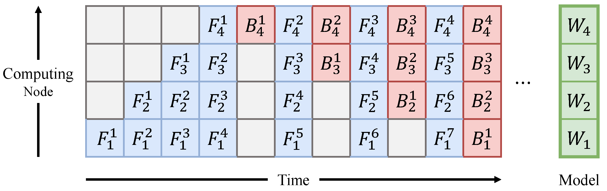
Pipelined SGD typically groups the layers of a DNN model into as many stages as the number of computing nodes and distributes the stages to the computing nodes (Figure 1). After the forward pass of the t-th mini-batch is completed at the layers in the n-th computing node, the $(n+1)$-th computing node proceeds with the next forward pass of the t-th mini-batch. At the same time, the n-th computing node simultaneously executes the forward pass of the $(t+1)$-th mini-batch. Similarly, all computing nodes simultaneously perform computations for different mini-batches in the backward pass as well. Therefore, pipelined SGD is suitable for large-scale DNN training because it uses all computing nodes without idle time and reduces the burden on each computing node, in terms of memory use, by dispersing the DNN model parameters.

However, when a backward pass is executed at a computing node in naive pipelined SGD, the forward pass values and the model parameters required for the backward pass computation have been changed already by a different mini-batch, causing the weight inconsistency problem (i.e., the model parameters used during the forward and backward passes are different). For example, the model parameters used in the forward pass of the second mini-batch in the third computing node (denoted as $F_3^2$ in Figure 1) and the resulting forward pass values are changed in the process of $F_3^3$ (the forward pass of the third mini-batch), $B_3^1$ (the backward pass of the first mini-batch), and $F_3^4$ (the forward pass of the fourth mini-batch). Hence, an incorrect forward pass values and stale weights are used for $B_3^2$, which is the backward pass of the second mini-batch in the third computing node, causing the delayed gradient problem in the naive pipeline parallelism. Previous works on pipelined SGD used the terms delayed gradient and weight inconsistency interchangeably. In this work, delayed gradient refers to the late-arriving gradients as in the ASGD algorithm, and weight inconsistency refers to the phenomenon that occurs in the naive pipeline parallelism, which is the cause of the delayed gradients.

Various approaches have been studied to solve the delayed gradient problem in pipelined SGD and improve the accuracies. In this section, the approximation methods analyzed in [17] are briefly described.

Decoupled parallel backpropagation using delayed gradient [18] executes the forward pass sequentially and uses the pipelining only for the backward pass. Though forward passes are executed correctly, since backward passes proceed simultaneously in a pipeline manner, the weight inconsistency problem persists. Also, there is a limit to improving the parallelization performance because the higher the number of computing nodes, the larger the effect of delayed gradients.

GPipe [19] executes the forward and backward passes by the pipeline method at a level of micro-batch, which a mini-batch is further divided. However, though the problem of weight inconsistency is solved, its convergence and parallelization efficiencies may decrease depending on the size of the mini-batch and the number of computing nodes because the backward passes start after all the forward passes have been finished, i.e., some computing nodes may not participate in the computation during the forward–to–backward and backward–to–forward transition periods.

DAPPLE [20] uses a gradient accumulation method in which the gradients of mini-batches are accumulated and the model parameters are updated once using the accumulated gradients. Though it avoids the weight inconsistency problem, this method has the effect of increasing the effective mini-batch size, thereby reducing the random walk phenomenon and lowering the accuracy of the DNNs.

SpecTrain [21] tries to prevent the weight inconsistency by predicting the future model parameters using the momentum technique and employing them in the forward and backward passes. Linear weight prediction [22] predicts the future model parameters using the momentum to circumvent the weight inconsistency problem as in SpecTrain. However, in these techniques, the higher the number of computing nodes, the more inaccurate the predicted model parameters become, resulting in limited parallelization efficiency.

PipeMare [23] tries to mitigate the weight inconsistency problem by using estimated forward pass model parameters at the time of the backward pass and alleviates the delayed gradient problem by using smaller values of the learning rate. However, it does not completely solve the weight consistency problem, so the more computing nodes there are, the more unstable the model convergence becomes.

Spike compensation [22] increases the contribution of the latest gradient in pipelined SGD with momentum. It has the effect that the overall contribution of each gradient matches the case of original SGD where weight inconsistencies do not occur. However, the training becomes unstable as the number of computing nodes increases.

FTPipe [24] is a pipeline parallelism proposed for fine-tuning pre-trained models. It does not mitigate the weight inconsistency problem with the assumption that the pre-trained models are less sensitive to weight staleness. However, not taking the staleness into account at all leads to an accuracy drop.

A potential solution for the weight inconsistency problem involves the creation of the same number of model replicas as that of time delays in the delayed gradient for each computing node and updating these replicas during the backward pass [25]. For example, PipeDream [26,27] uses this method, with the name of weight stashing. Furthermore, the same number of model replicas as the largest number of delay occurrences at all computing nodes can be created such that all computing nodes can use the same previous time step parameters during the backward passes. It is called vertical sync in PipeDream [26]. This method can be considered as the combination of model parallelism and data parallelism. Therefore, additional synchronization of model parameters is required.

3. Proposed Methods

3.1. Pipelined SGD Work Scheduling and Model Replicas for the Proposed Methods

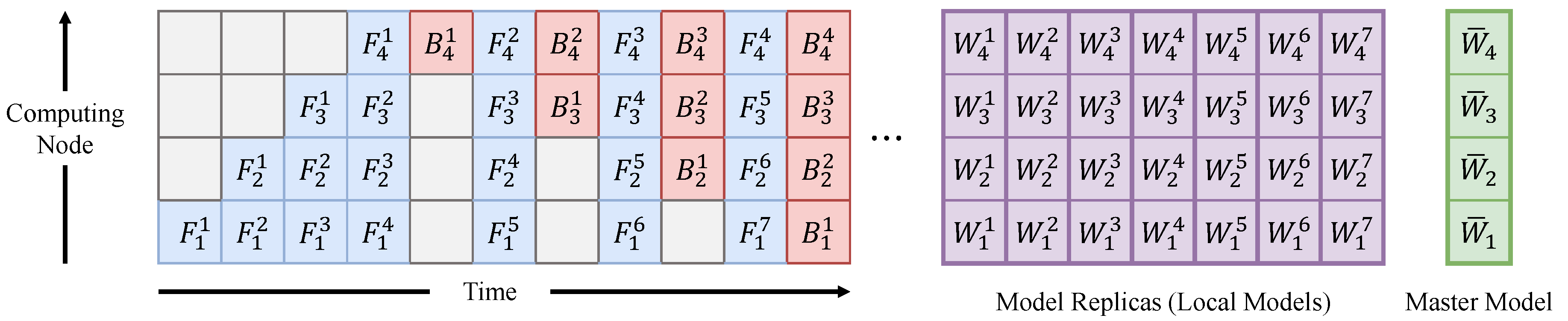
The proposed work scheduling for pipelined SGD is depicted in the left part of Figure 2. It shows the simultaneous execution of forward or backward passes for different mini-batches. For example, when the forward pass of the 5th mini-batch is executed in the 2nd computing node (denoted as $F_2^5$), the forward pass of the 6th mini-batch is executed concurrently in the first computing node (denoted as $F_1^6$). Similarly, $B_2^1$, which denotes the backward pass of the 1st mini-batch in the second computing node, and $B_3^2$, which denotes the backward pass of the 2nd mini-batch in the 3rd computing node, are executed in parallel.

The master model and the model replicas required to prevent the weight inconsistency problem caused by the naive pipelined SGD are shown in the right part of Figure 2. The proposed pipelined SGD creates $2N-1$ model replicas when the number of computing nodes is N. In Figure 2, for example, seven model replicas are created for the pipelined SGD with four computing nodes. To access the model parameters used in $F_3^3$ (the forward pass of the 3rd mini-batch in the 3rd computing node) and the output values of $F_3^3$ when $B_3^3$ (the backward pass of the 3rd mini-batch in the 3rd computing node) is executed, the model parameters used in $F_3^3$ must not be changed during the backward passes from $B_3^1$ to $B_3^2$, and the output values of $F_3^3$ must not be changed after forward passes $F_3^4$ and $F_3^5$. Therefore, three sets of model parameters of different time points ($W_3^3$, $W_3^4$, and $W_3^5$) must be maintained at the 3rd computing node until $B_3^3$ is executed. Also, three sets of output values from $F_3^3$, $F_3^4$, and $F_3^5$ must be maintained. Similarly, seven sets of model parameters ($W_1^1$, $W_1^2$, ..., $W_1^7$) of different time points and seven sets of output values from $F_1^1$, $F_1^2$, ..., $F_1^7$ must be maintained until $B_1^1$ is executed at the first computing node. To support data parallelism, however, $2N-1$ sets of model parameters and output values of different time points must be maintained at every computing node because any local model replica of the same time point as the one in the first computing node should be accessible in each computing node. Since $2N-1$, different DNN models use different mini-batches in parallel training, and data parallelism occurs as well as model parallelism in the proposed pipelined SGD. In this case, the master model corresponds to the model of the parameter server in ASGD; by contrast, in the proposed pipelined SGD, each stage of the master model is separately stored at each computing node by model parallelism (${\overline{W}}_1$, ${\overline{W}}_2$, ${\overline{W}}_3$, and ${\overline{W}}_4$ in Figure 2).

Combining these $2N-1$ model replicas to produce the master model can be performed using data parallelism techniques. ASGD algorithms have many advantages over SSGD, including efficiency and error resilience, so these ASGD algorithms can be applied to combine model replicas. However, direct use of ASGD induces the delayed gradient problem, as in the original data parallelism algorithms. Therefore, we propose a new pipelined SGD algorithm, TaylorPipe, which applies the Taylor expansion to mitigate the delayed gradient problem of the naive pipeline parallelism.

3.2. Pipelined SGD with Taylor Expansion (TaylorPipe)

To alleviate the delayed gradient problem occurring in ASGD, the gradient at a future point in time may be approximated by applying the Taylor expansion [15]. As gradients are the first-order derivatives of the loss function, the second-order derivatives should be used in applying the Taylor expansion. To predict the gradient of the master model ${\overline{W}}_n$ that is from the future in time using the current time local model $W_n^t$, the following Taylor expansion can be used:

$$\begin{array}{c}\hfill \nabla \mathcal{L}({\overline{W}}_n;x^t,y^t)=\nabla \mathcal{L}(W_n^t;x^t,y^t)+{\nabla }^2\mathcal{L}(W_n^t;x^t,y^t)({\overline{W}}_n-W_n^t)+\epsilon ,\end{array}$$

(2)

where $\epsilon$ is the error caused by the first-order Taylor expansion. The Hessian matrix, which is the second-order derivative of the loss function, can be approximated using an appropriate value of $\lambda$ as follows [15]:

$$\begin{array}{c}\hfill {\nabla }^2\mathcal{L}(W_n^t;x^t,y^t)\approx \lambda \nabla \mathcal{L}(W_n^t;x^t,y^t)\odot \nabla \mathcal{L}(W_n^t;x^t,y^t),\end{array}$$

(3)

where ⊙ represents the pair-wise dot product.

The proposed TaylorPipe alternately performs the forward pass and backward pass according to the work scheduling in Figure 2. Each computing node calculates the Taylor expansion only for the stage of the model assigned to the computing node, instead of for the entire model, because the pipelined SGD work scheduling and the model replicas described in Section 3.1 allow model parallelism as well as data parallelism.

A pseudo-code of TaylorPipe is presented in Algorithm 1, which is executed by all computing nodes simultaneously. In the algorithm, $t_{\mathrm{f}}$ and $t_{\mathrm{b}}$ represent the mini-batch indices for the forward and backward passes, respectively, and T denotes the total number of mini-batches. During the initial and final phases, only the forward and backward passes are executed, respectively. After the $(n+1)$-th computing node finishes executing the backward pass $B_{n+1}^{t_{\mathrm{b}}}$, the n-th computing node calculates the gradient in the backward pass $B_n^{t_{\mathrm{b}}}$ using the local model $W_n^{t_{\mathrm{b}}}$ for the mini-batch of index $t_{\mathrm{b}}$. Subsequently, it performs the Taylor expansion of the gradient for the master model ${\overline{W}}_n$, and the updated master model is copied back to the local model. At a given time point, each stage of the master model in the computing nodes contains the updated model parameters trained on different mini-batches. For example, when $B_1^1$ and $B_2^2$ are finished, ${\overline{W}}_1$ and ${\overline{W}}_2$ contain the model parameters trained using up to the 1st and 2nd mini-batches, respectively. However, when the pipeline is flushed completely, all stages of the master model in the computing nodes finally contain the model parameters of the same time version.

Algorithm 1 TaylorPipe: Executed by computing node n in parallel with all other computing nodes.

In the proposed method, the master model and local model are stored in the memory of the same computing node. Hence, TaylorPipe does not need to have additional memory for the backup model nor to copy the gradients to the parameter server, unlike in the conventional ASGD. That is, compared with the conventional ASGD employing Taylor expansion, TaylorPipe has the advantage of less memory requirement and less communication cost when updating the model parameters. Furthermore, the bottleneck phenomenon due to simultaneous access to the master model does not occur because the local models stored in each computing node are sequentially synchronized with the master model.

3.3. Computation and Communication Complexities

In this section, we analyze and compare the computation complexity and communication complexity of SSGD, ASGD, and TaylorPipe [17]. Let H denote the number of neurons in a layer, which is assumed to be the same for all layers in a fully connected DNN model. L represents the number of layers in the model, M indicates the number of instances in a mini-batch, and T is the number of mini-batches in the training data. The computation complexity of the vanilla SGD for one epoch is $\mathsf{𝒪}\left(H^{2}LMT\right)$.

When N computing nodes are used in parallel, the computation complexity for SSGD and ASGD on each computing node is $\mathsf{𝒪}\left(H^{2}LMT/N\right)$ since each computing node processes $T/N$ mini-batches. In ASGD, as the parameter server updates the master model after each mini-batch, it requires $\mathsf{𝒪}\left(H^{2}LT\right)$ operations. On the other hand, it requires $\mathsf{𝒪}\left(H^{2}LT/\kappa \right)$ operations for the master model update in SSGD, as the parameter server updates the master model after every $\kappa$ mini-batches. In TaylorPipe, each computing node processes all T mini-batches, but only for $L/N$ layers, so the computation complexity becomes $\mathsf{𝒪}\left(H^{2}LMT/N\right)$, which is the same as the cases of SSGD and ASGD. However, TaylorPipe does not require additional model synchronization because each computing node updates the master model directly.

The model synchronization in ASGD and SSGD requires the communication between the parameter server and all N computing nodes. Therefore, the communication complexity of ASGD is $\mathsf{𝒪}\left(H^{2}LT\right)$, while that of SSGD is $\mathsf{𝒪}\left(H^{2}LT/\kappa \right)$. On the other hand, since the master model and local models reside in the same computing nodes, no communication is required for the model synchronization in TaylorPipe. However, the results of the forward and backward passes are transmitted to the adjacent computing nodes in parallel, which results in the communication complexity of $\mathsf{𝒪}\left(HMT\right)$.

The computation and communication complexities of SSGD, ASGD, and TaylorPipe are summarized in

Table 1. The computation and communication complexities of SSGD, ASGD, and TaylorPipe for training a fully connected DNN model using N computing nodes. H denotes the number of neurons in each layer, L represents the number of layers in the model, M indicates the number of instances in each mini-batch, and T is the number of mini-batches in the training data.

Method	Computation Complexity (Computing Node)	Computation Complexity (Parameter Server)	Communication Complexity
SSGD	$\mathsf{𝒪}(H^{2}LMT/N)$	$\mathsf{𝒪}(H^{2}LT/\kappa )$	$\mathsf{𝒪}(H^{2}LT/\kappa )$
ASGD	$\mathsf{𝒪}(H^{2}LMT/N)$	$\mathsf{𝒪}\left(H^{2}LT\right)$	$\mathsf{𝒪}\left(H^{2}LT\right)$
TaylorPipe	$\mathsf{𝒪}(H^{2}LMT/N)$	-	$\mathsf{𝒪}\left(HMT\right)$

. Though the computation complexities in a computing node for all three methods are the same, TaylorPipe has the advantage in communication, since $HM$ is usually much smaller than $H^{2}L/\kappa$ in a large-scale DNN training.

4. Experiments

Experiments were conducted to analyze the efficiency of the proposed pipelined SGD method by comparing it with the conventional parallel SGD algorithms in terms of the accuracy and training speed on an image classification task using two datasets: CIFAR-10 and CIFAR-100. VGG-16 [16] and ResNet-34 [9] were used as the DNN models for the image classification experiments. The training algorithms used in the comparative study include the conventional sequential SGD (denoted as SGD), the naive pipelined SGD that condones the weight inconsistency (denoted as NaivePipe), PipeDream [26], SpecTrain [21], and TaylorPipe. In order to analyze the effect of the weight inconsistency and delayed gradient problems only and compare the conventional methods with the proposed methods fairly, PipeDream and SpecTrain used the same work scheduling and model replicas as TaylorPipe, which were explained in Section 3.1. Our implementation of PipeDream computes the master model parameters by calculating the average of the local model parameters at every model synchronization period. Since this effectively becomes one of the SSGD methods, the delayed gradient problem does not occur. We implemented the aforementioned algorithms using the DNN library provided by the Compute Unified Device Architecture and compared their performance under the same hardware conditions. The performance of each algorithm was evaluated with a varying number of GPUs (one, two, four, and eight) on a server with eight NVIDIA RTX 2080 Ti GPUs. We conducted experiments five times with a different random seed and reported the best case. An image augmentation technique was applied to prevent overfitting. 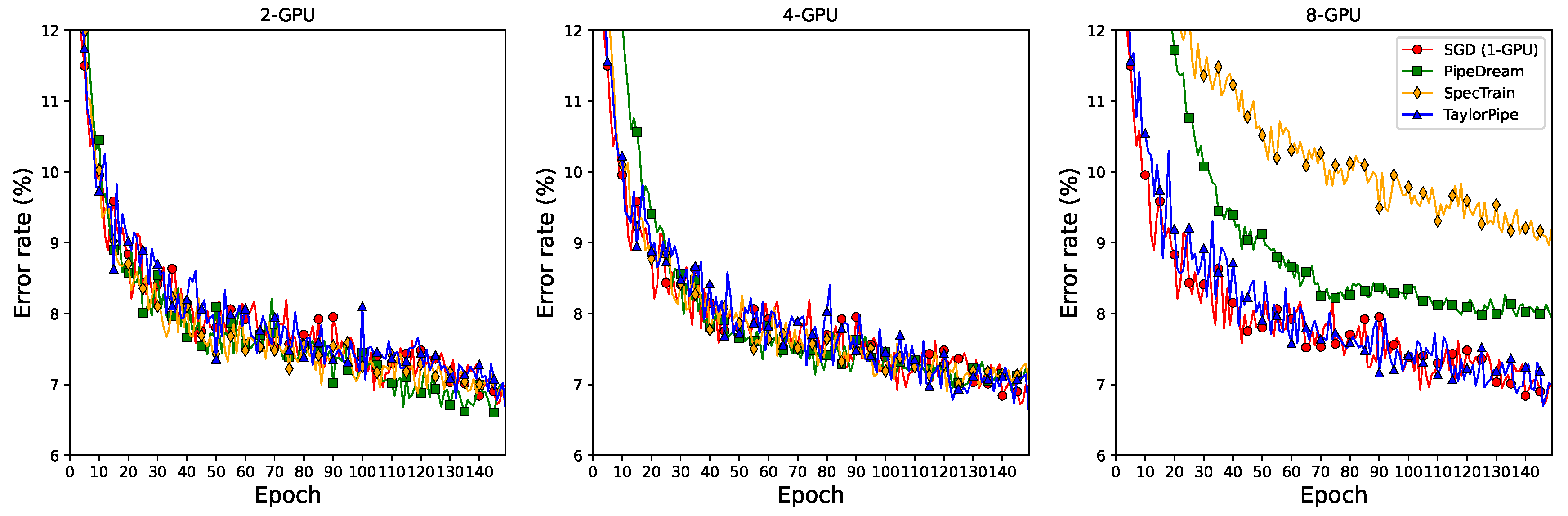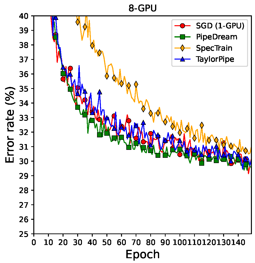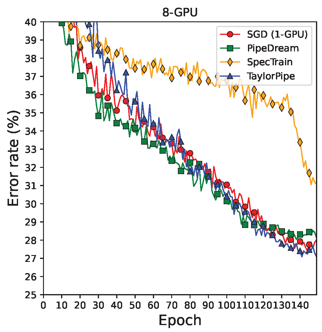The hyperparameter settings for experiments can be found in Appendix A. The test error rate curves can be found in Appendix B.

Table 2. Image classification error rate (%) and training time (in hours) of each method using the CIFAR-10 dataset and the VGG-16 model for various numbers of GPUs.

Algorithm	Error Rate (%)				Training Time (Hours)
	1-GPU	2-GPU	4-GPU	8-GPU	1-GPU	2-GPU	4-GPU	8-GPU
SGD	6.73	-	-	-	11.96	-	-	-
NaivePipe	-	72.07	74.18	81.70	-	0.10	0.06	0.05
PipeDream	-	6.61	6.93	7.95	-	7.89	4.95	4.64
SpecTrain	-	7.03	7.07	7.43	-	7.86	5.30	4.65
TaylorPipe	-	6.64	6.63	6.70	-	8.35	5.26	4.51

shows the image classification error rate and training time of each training method using the CIFAR-10 dataset and the VGG-16 model for various numbers of GPUs. SGD shows the error rate of 6.73%. NaivePipe failed to converge because it does not cope with the weight inconsistency and delayed gradient problems. Both of the conventional pipelined SGD methods (PipeDream and SpecTrain) and the proposed pipelined SGD method (TaylorPipe) show similar error rates to SGD when two GPUs are used. However, the error rates increase as the number of GPUs used increases. Since PipeDream uses one of the SSGD methods, which increases the effective mini-batch size by the number of computing nodes, the enlarged effective mini-batch size will degrade the DNN model training. SpecTrain predicts the future model parameters to prevent the weight inconsistency, but the greater the number of computing nodes, the more inaccurate the predicted model parameters become, resulting in limited DNN model training. However, TaylorPipe shows stable performance regardless of the number of GPUs used. We suspect that the simple averaging method and the momentum-based future model prediction scheme are not as effective as the Taylor expansion-based future gradient prediction, in mitigating the delayed gradient problem.

Another important factor that affects the overall training time is statistical efficiency, i.e., the number of epochs required to reach a desired level of accuracy. Since NaivePipe failed to converge, it finished early. In the eight-GPU experiments, SpecTrain and PipeDream are the slowest and the second slowest among the parallel algorithms and their error rates are much higher than the proposed methods. TaylorPipe not only shows the comparable error rate with SGD but also is 2.6 times faster than SGD.

Table 3. Average training time (in seconds) per epoch for each method using the CIFAR-10 dataset and the VGG-16 model for various numbers of GPUs.

Algorithm	1-GPU	2-GPU	4-GPU	8-GPU
SGD	293	-	-	-
NaivePipe	-	187	118	107
PipeDream	-	194	123	111
SpecTrain	-	213	129	112
TaylorPipe	-	200	126	110

shows the averaging training time per epoch for each method using the CIFAR-10 dataset and the VGG-16 model for various numbers of GPUs. For all parallel algorithms, the average training time per epoch decreases in proportion to the number of GPUs used. NaivePipe is the fastest because it does not perform any extra work to handle the weight inconsistency and delayed gradient problems. PipeDream is faster than SpecTrain because the synchronization period was set to be somewhat large. TaylorPipe is faster than SpecTrain since the number of operations for gradient prediction is smaller than the number of operations for weight prediction, i.e., TaylorPipe predicts the gradients during the backward pass only whereas SpecTrain predicts the weights both for the forward and backward passes. For all parallel algorithms, as the number of GPUs used increases, the effect of extra computation time to handle the weight inconsistency and delayed gradient problems diminishes and the overhead of communication time overwhelms, leading to comparable training time per epoch in the last column of Table 3.

Table 4. Image classification error rate (%) and training time (in hours) of each method using the CIFAR-100 dataset and the VGG-16 and ResNet-34 models on 8 GPUs.

Algorithm	Error Rate (%)		Training Time (Hours)
	VGG-16	ResNet-34	VGG-16	ResNet-34
SGD	29.14	27.42	12.20	22.77
PipeDream	29.38	28.04	4.70	13.11
SpecTrain	30.50	31.05	4.60	9.28
TaylorPipe	29.46	27.09	4.43	8.69

shows the image classification error rate and training time of of each method using the CIFAR-100 dataset and the VGG-16 and ResNet-34 models on eight GPUs.

In the VGG-16 experiment, the training time for PipeDream to reach the minimum error rate is the slowest among the pipelined SGD algorithms. SpecTrain is the one of the slowest algorithms and shows the worst error rate. The proposed method, TaylorPipe, shows comparable error rates to SGD, with about 2.7 times faster convergence speed.

In the ResNet-34 experiment, PipeDream shows the slowest training time to reach the minimum error rate among the parallel algorithms. Since the synchronization period of PipeDream was set to 1, PipeDream should flush the pipeline more frequently to synchronize the master model with local models. It not only increases the training time per epoch but also uses computing nodes inefficiently. These are the major drawbacks of the pipelined SGD using the SSGD method. SpecTrain shows the second slowest training time and achieves the worst error rate of 31.05%. TaylorPipe shows the fastest training time among the parallel algorithms. Compared to SGD, the training time of TaylorPipe is 2.6 times faster. Furthermore, TaylorPipe recorded a similar error rate to that of SGD.

Based on our experiments, the proposed method, TaylorPipe, shows robust performance in terms of both image classification error rate and the training time to reach the minimum error rate. Therefore, it can be inferred that TaylorPipe not only overcomes the weight inconsistency problem but also more efficiently alleviates the delayed gradient that occurs in the pipelined SGD.

5. Conclusions

In this study, a novel pipelined parallel SGD algorithm, TaylorPipe, is proposed to mitigate the weight inconsistency and delayed gradient problems that occur when implementing the inherently sequential SGD algorithm as pipeline parallelism to improve the training speed. It generates multiple model replicas to address the weight inconsistency problem and predicts gradients by using Taylor expansion to alleviate the delayed gradient problem. The experimental results confirmed that the convergence rate does not decrease even if the number of computing nodes increases, unlike in the conventional parallel SGD algorithms. Therefore, the proposed method is expected to train DNN models more efficiently in a large-scale parallel processing environment. Furthermore, the attempted combination of pipeline parallelism and data parallelism in this paper will serve as an example advising diverse approaches to address issues that arise during parallelizing deep learning. However, the proposed method has a disadvantage in terms of memory efficiency because it creates multiple model replicas. For future work, we believe that applying memory optimization techniques in deep learning, such as gradient accumulation, gradient checkpointing, or mixed precision methods, and so on, may be explored to effectively address this problem.