Article

Non-Parametric Calibration of the Inverse Kinematic Matrix of a Three-Wheeled Omnidirectional Mobile Robot Based on Genetic Algorithms

Robotics Laboratory, Universitat de Lleida, Jaume II, 69, 25001 Lleida, Spain
*
Author to whom correspondence should be addressed.
Appl. Sci. 2023, 13(2), 1053; https://doi.org/10.3390/app13021053
Submission received: 16 December 2022 / Revised: 4 January 2023 / Accepted: 10 January 2023 / Published: 12 January 2023
(This article belongs to the Special Issue Advances in Robot Path Planning, Volume II)

Abstract

:

Featured Application

Odometry calibration of a three-wheeled omnidirectional mobile robot.

Abstract

Odometry is a computation method that provides a periodic estimation of the relative displacements performed by a mobile robot based on its inverse kinematic matrix, its previous orientation and position, and the estimation of the angular rotational velocity of its driving wheels. Odometry is cumulatively updated from tens to hundreds of times per second, so any inaccuracy in the definition of the inverse kinematic matrix of a robot leads to systematic trajectory errors. This paper proposes a non-parametric calibration of the inverse kinematic (IK) matrix of a three-wheeled omnidirectional mobile robot based on the use of genetic algorithms (GA) to minimize the positioning error registered in a set of calibration trajectories. The application of this non-parametric procedure has provided an average improvement of 82% in the estimation of the final position and orientation of the mobile robot. This is similar to the improvement achieved with analogous parametric methods. The advantage of this non-parametric approach is that it covers a larger search space because it eliminates the need to define feasible physical limits to the search performed to calibrate the inverse kinematic matrix of the mobile robot.

1. Introduction

Odometry is a direct computation method that provides a periodic estimation of the relative displacement of a mobile robot through the use of its inverse kinematic matrix, its previous orientation and position, and the estimation of the angular rotational velocity of its driving wheels. Odometry is cumulatively updated from tens to hundreds of times per second so any inaccuracy in the definition of the inverse kinematic matrix of the robot causes systematic trajectory estimation errors. Borenstein et al. [1] proposed the University of Michigan Benchmark (UMBmark) test to estimate and correct systematic odometry errors in differential drive mobile robots. The existence of systematic odometry errors in a differential drive mobile robot is usually evidenced when a straight trajectory becomes curved. The UMBmark defines a motion experiment in which a differential drive mobile robot follows a square-shaped path in either a clockwise or counterclockwise direction in order to provide unbiased error compensations in both directions. The UMBmark test assumes that systematic odometry errors are caused by an inaccurate definition of the distance from the wheels to the center of rotation of the mobile robot and by an inaccurate definition of the diameters of the wheels. However, the trajectory of the mobile robot may also be conditioned by such other parameters as the controllers driving its motors [2,3,4]. The effects of all the error sources in the odometry of the mobile robot are usually summarized in the computation of its effective inverse kinematics [5].
Compared with non-holonomic robots, odometry estimation in omnidirectional mobile robots is far more complex due to their enhanced motion capabilities. The additional degrees of freedom offered by omnidirectional robots, along with a larger number of parameters involved in the definition of their kinematic models, can accentuate the effects of systematic errors [6,7]. In the case of a three-wheeled omnidirectional motion system, Maddahi et al. [8] proposed a method to reduce odometry errors based on the application of two corrective indices to the inverse kinematic matrix of the robot. In summary, the application of these two corrective indices has the effect of correcting the angular velocities of the wheels, which can be considered equivalent to a parametric calibration of the radii of the wheels. Maddahi et al. [8] concluded that the application of these corrective indices provides better error reduction in the case of the mobile robot performing straight trajectories rather than curved trajectories. Alternatively, Lin et al. [9] proposed a method to reduce odometry errors based on the direct correction of the kinematic model of an omnidirectional mobile robot using different calibration trajectories. Similarly, the inverse kinematics and trajectory performance of four-wheeled omnidirectional mobile robots have been specifically analyzed by different authors. Maulana et al. [10] analyzed the inverse kinematics in a mecanum mobile robot using stepper motors. Jia et al. [11] analyzed the kinematic model of a mecanum wheeled robot with four wheels. Xu et al. [12] analyzed the tracking performance of a four-wheeled omnidirectional mobile robot using sliding mode control. Li et al. [13] proposed a procedure to reduce odometry errors by considering the problem of wheel slippage due to the motion constraints originated by wheel redundancy in four-wheeled omnidirectional mobile robots. In this case, Li et al. [13] proposed the determination of a non-parametric velocity compensation matrix that is applied to the kinematic model of the mobile robot with the objective of reducing the specific odometry error caused by wheel slippage. In a similar direction, Savaee et al. [14] proposed a non-parametric approach to calibrate the effective kinematic matrix of an omnidirectional mobile robot. This proposal was based on the comparison of trajectory simulations, performed with a virtual mobile robot, with experimental trajectory measurements performed by the real mobile robot. Under such conditions, the assumption was that offline calibration of the kinematic matrix of the mobile robot was less prone to local minima effects [15]. Prados et al. [16] analyzed the motion performance of a four-wheeled omnidirectional mobile robot tailored for surveillance application in limited spaces.
Finally, in a previous work [17], we performed the parametric optimization of the inverse kinematic matrix of a real three-wheeled omnidirectional mobile robot. This approach was based on the definition of a set of benchmark omnidirectional trajectories and an offline parametric optimization based on odometry computation. The parameters analyzed as possible error sources were: the radius of the three omnidirectional wheels, the distance from the wheels to the center of rotation of the mobile robot and the angular orientation of the wheels. These nine parameters (three error sources for each of the three wheels) were iteratively calibrated in order to optimize the inverse kinematic matrix that defines the odometry of the mobile robot. The underlying hypothesis of this parametric optimization was the possibility of directly identifying assembling imprecisions originated during the construction of the robot and thus being able to correct the cause of systematic errors in the trajectory of the robot. However, the analysis of the results obtained in [17] showed that the calibrated values of the parameters have no direct feasible interpretation in the mobile robot. For example, the diameter of the wheels that improves the odometry does not correspond to the wheel diameters obtained with accurate measurements.

New Contribution

This paper proposes a non-parametric calibration of the inverse kinematic (IK) matrix of a three-wheeled omnidirectional mobile robot. This calibration procedure is based on the multidimensional search capabilities of genetic algorithms (GA), which are used to iteratively fit a numerical description of the inverse kinematic matrix that improves the odometry of a three-wheeled omnidirectional mobile robot.
Genetic algorithm optimization has many practical applications in robotics [18,19,20,21,22]. In this paper, genetic optimization is applied in an offline procedure that recomputes the odometry from the mobile robot data registered in 36 representative straight and curved trajectories. These trajectories were inspired by the proposal of Maddahi et al. [8] and Batlle et al. [23] and were already proposed in [17] as a benchmark for offline omnidirectional mobile robot calibration.
The performance of the experimental application of this non-parametric calibration procedure in a real three-wheeled omnidirectional mobile robot has been evaluated in terms of odometry improvement. The main advantage of this non-parametric calibration procedure, relative to a parametric calibration [17], is that it does not require the definition of feasible physical-interpretable limits during the iterative search performed by genetic algorithms. As a result, the search space is larger but the iterative calibration procedure converges faster. The main theoretical disadvantage of this non-parametric calibration procedure is the leak of feasible physical interpretation of the fitted inverse kinematic matrix (such as wheel diameter, distance of the wheel, etc.), although a previous work [17] showed that the result of a parametric calibration cannot be physically interpreted.

2. Materials and Methods

The materials and methods used in this paper are: the APR-02 three-wheeled omnidirectional mobile robot, the method used to compute the odometry of the mobile robot, the representative calibration trajectories, and the dataset of training and validation trajectories used to calibrate the inverse kinematic matrix of this mobile robot.

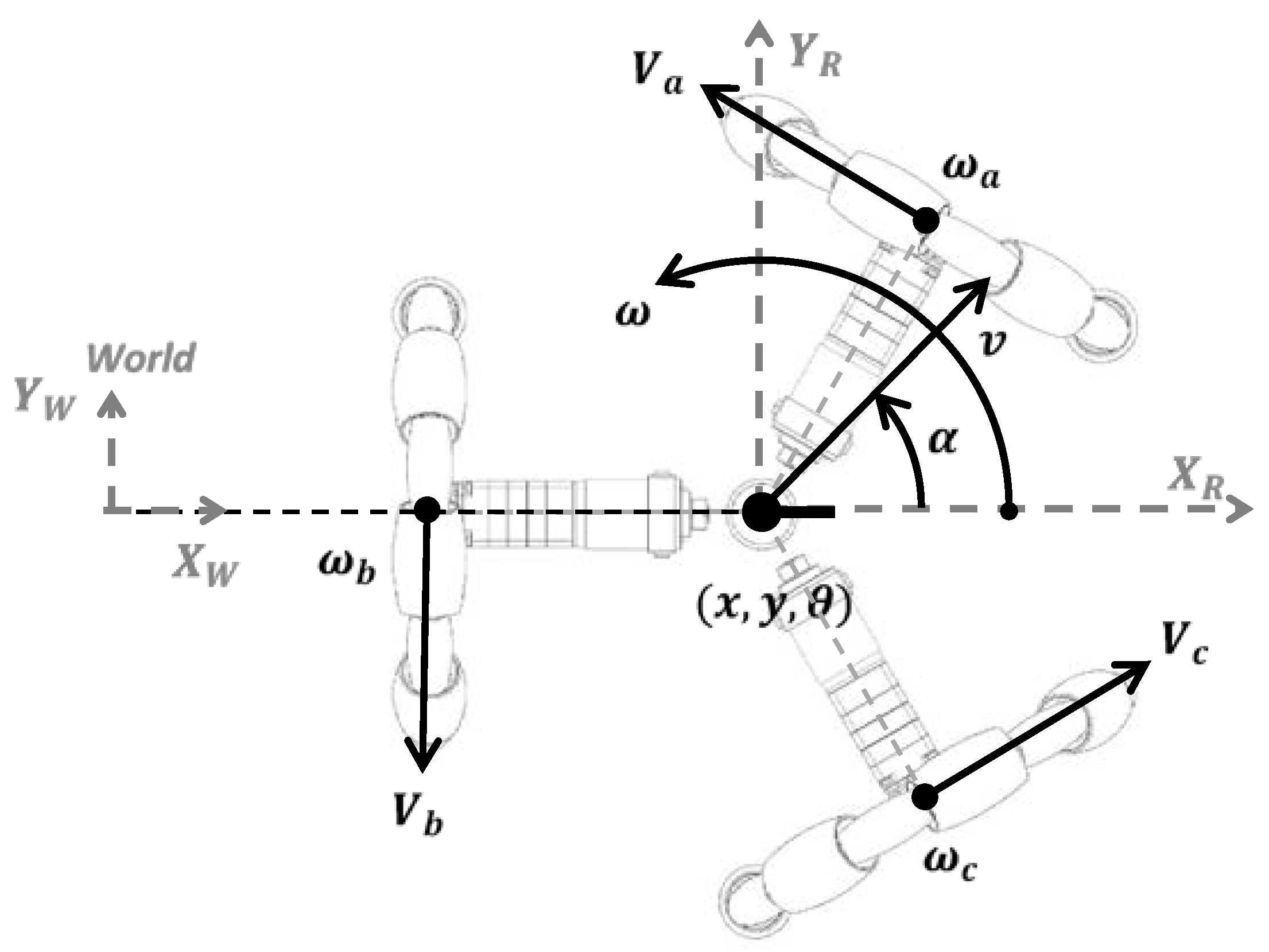
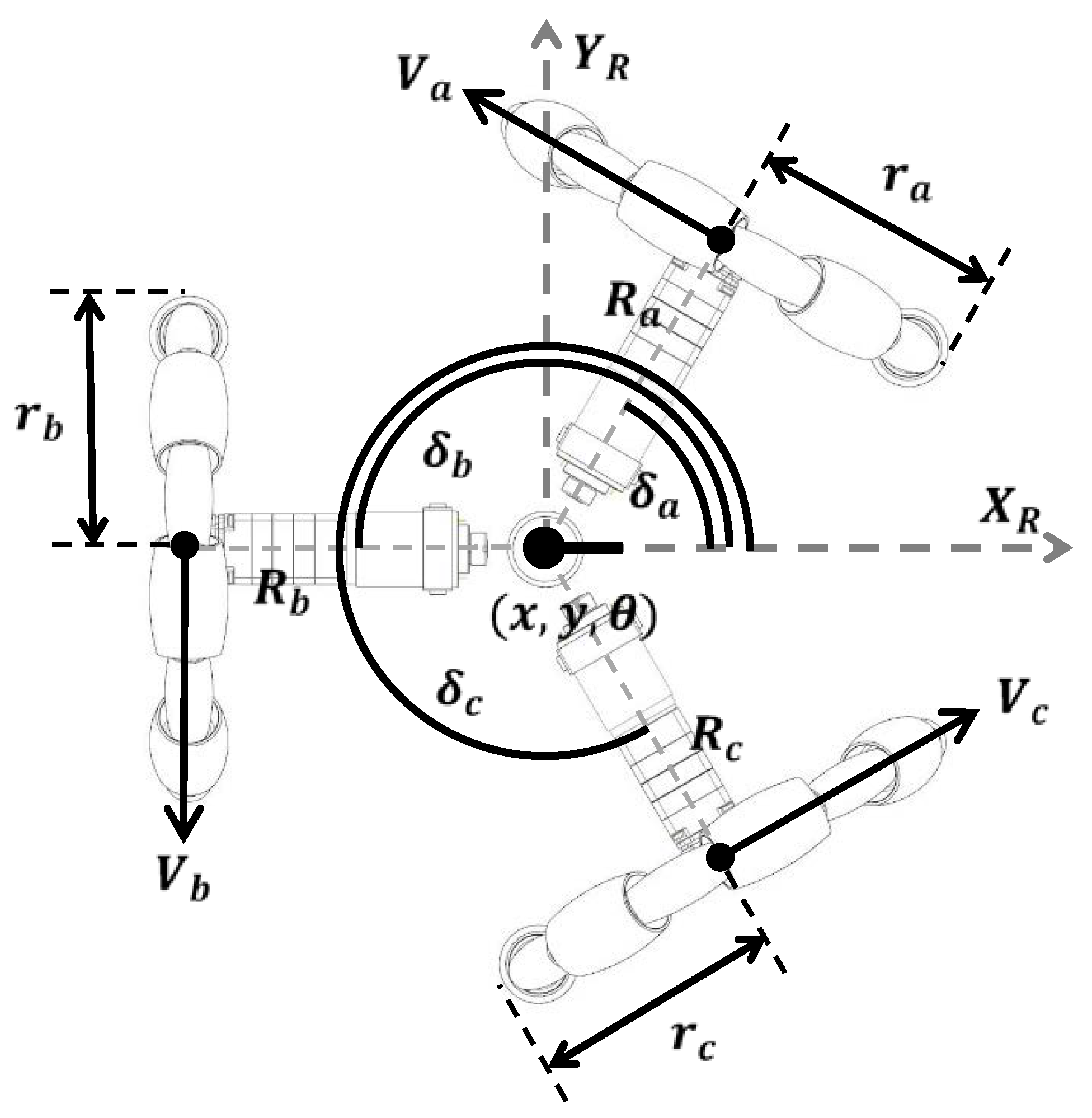
2.1. APR-02 Three-Wheeled Omnidirectional Mobile Robot

The robot assessed in this paper is the autonomous APR-02 three-wheeled omnidirectional robot, which was initially devised as a mobile telepresence platform [24]. The inclusion of an onboard high-end computer in the following prototypes allowed the development of autonomous applications, e.g., supporting and guiding older people with mobility impairments [25], and an early gas leak detection system [26]. The main characteristic of this assistive mobile robot [27] is the use of an omnidirectional motion system based on three optimal omnidirectional wheels [28] driven by three brushed direct current motors (BDCM) [29]. The odometry of the robot is calculated from the information provided by the encoders of the motors. The advantage of a three-wheeled against a four-wheeled omnidirectional motion system is the avoidance of wheel slippage [17,30].
Figure 1 shows some images of the APR-02 mobile robot completing a displacement. The trajectory of the mobile robot is controlled by a target motion command ( v , α , ω , t r ) [30] that defines: the translational velocity of the motion ( v ); the angular orientation of the planned motion ( α ), defined in a complete range from 0° to 360°; the angular rotational speed of the base of the mobile robot ( ω ) while performing a displacement; and the time duration of this motion command ( t r ), which can be replaced by a target distance displacement. The path planning algorithm of the mobile robot periodically updates the target motion command every 300 ms. The maximum value of the time duration ( t r ) is always lower than 500 ms as a kind of watchdog security measure to stop the mobile robot automatically in case of malfunction of its central processing unit. This omnidirectional mobile robot is able to move in any angular orientation ( α ) without having to perform any previous maneuver, also being able to rotate over itself while moving [30].
The determination of the ground truth trajectory of the mobile robot is based on the application of SLAM [31] to the precise information gathered from its onboard Hokuyo UTM-30LX 2D LIDAR, which is placed horizontally or tilted down [32] depending on the expected surrounding environment. The practical disadvantage of using a high-precision LIDAR is its high cost. There are also other cheaper positioning alternatives that have been proven useful for kinematic calibration [33] and in the application of mobile robots intended to operate in the presence of dynamic obstacles, such as people [34].

2.2. Odometry Estimation

Odometry is a computation method that provides a periodic estimation of the relative displacement of a mobile robot. This computation requires an accurate and precise definition of its inverse kinematic matrix, its previous position and orientation, and the estimation of the angular rotational velocities of its driving wheels. The consequence of any inaccuracy or imprecision is the generation of systematic odometry errors. Additionally, odometry interprets the angular rotational speeds of the wheels of the mobile robot as linear displacements, so it requires non-slippage wheel conditions throughout the trajectory. In the case of a three-wheeled omnidirectional mobile robot, the wheels have no motion constraints and no slippage is originated while performing any continuous motion [30].
The kinematics and the odometry of a three-wheeled omnidirectional mobile robot such as the APR-02, was described previously in [17,30]. This practical odometry estimation is challenging because of the degree of freedom provided by its omnidirectional motion system. Figure 2 presents the definition of the omnidirectional motion system of the APR-02 mobile robot: ( x , y , θ ) is the position of the mobile robot referred to the absolute or fixed world frame ( X W , Y W ) , ( X R , Y R ) is the relative mobile robot frame, ( v , α , ω ) is the motion command that specifies the target trajectory planned for the mobile robot, ( ω a , ω b , ω c ) are the angular velocities of the wheels required to implement the motion command, and ( V a , V b , V c ) are the deduced linear velocities of the wheels.
Odometry uses the instantaneous estimate of the current angular velocities of the three wheels, a ,   b ,   c , given as ( ω a ( k ) , ω b ( k ) , ω c ( k ) ) , and defined in rad/s; and the previous position of the mobile robot ( x ( k 1 ) , y ( k 1 ) ,   θ ( k 1 ) ) , defined in the absolute world frame ( X W , Y W ) . Both values are used to update the current position of the mobile robot ( x ( k ) , y ( k ) , θ ( k ) ) by using the following expression [17]:
[ x ( k ) y ( k ) θ ( k ) ] W o r l d = [ x ( k 1 ) y ( k 1 ) θ ( k 1 ) ] W o r l d + Δ t · R ( θ ( k 1 ) ) 1 · M 1 · [ ω a ( k ) ω b ( k ) ω c ( k ) ]
where Δ t is the sampling time at which the angular velocities of the wheels of the robot are updated and k is the current discrete sample number that describes a time elapsed t ( k ) (where t ( k ) = Δ t · k ) since the initialization of the robot. In the case of the APR-02, this sampling time coincides with the sampling time used internally by the three proportional, integral, and derivative (PID) controllers ( Δ t = 10   ms ) [29] of the three brushed direct current motors (BDCM) driving its three omnidirectional wheels.
In Equation (1), R ( θ ( k 1 ) ) 1 is the inverse of the rotation matrix computed from the previous instantaneous angular orientation of the mobile robot θ ( k 1 ) :
R ( θ ( k 1 ) ) 1 = [ cos ( θ ( k 1 ) )   sin ( θ ( k 1 ) ) 0 sin ( θ ( k 1 ) ) cos ( θ ( k 1 ) ) 0 0 0 1 ]
and M 1 is the inverse of the compact kinematic matrix of the mobile robot that can be computed analytically as [17]:
M 1 = 1 R a sin δ b δ c R b sin δ a δ c + R c sin δ a δ b · r a R b cos δ c R c cos δ b r b R a cos δ c R c cos δ a r c R a cos δ b R b cos δ a r a R b sin δ c R c sin δ b r b R a sin δ c R c sin δ a r c R a sin δ b R b sin δ a r a sin δ b δ c r b sin δ a δ c r c sin δ a δ b
where ( r a , r b , r c ) are the radii of the wheels, ( R a , R b , R c ) are the distances between the center of the robot and the wheels, and ( δ a , δ b , δ c ) are the angular orientations of the wheels defined in the mobile robot frame ( X R , Y R ) . Figure 3 presents the definition of all these parameters involved in the omnidirectional motion system of the APR-02. These have the following design values: r a , b , c = 0.148   m , R a , b , c = 0.195   m , δ a = 60 ° , δ b = 180 ° , δ c = 300 ° .

2.3. Calibration Trajectories

The calibration trajectories used in this paper are the same 36 representative benchmark trajectories proposed in [17]. These trajectories were proven useful for improving the odometry of a three-wheeled omnidirectional mobile robot [17]. The motion commands required to generate the calibration trajectories are listed in Table A1 of [17]. These benchmark trajectories define a characteristic flower-shaped figure that is representative of the motion capabilities of an omnidirectional mobile robot.
Table 1 lists the information registered by the APR-02 mobile robot while performing a calibration trajectory defined by a motion command ( v , α , ω ) , executed over a predefined distance or time. The path-planning algorithm of the mobile robot converts this target motion into the target angular rotational velocities ( ω M a , ω M b , ω M c ) to be applied to the three PID controllers [29] that supervise the motors of the robot. The main information registered in Table 1 is the complete sequence of angular rotational velocities of the wheels measured during a displacement, ω a , b , c . This information is used by the mobile robot to compute the odometry in real-time, but the registration of this information allows future offline re-computation of the odometry with a different inverse kinematic matrix (allowing its calibration). The APR-02 also estimates its position by applying SLAM to the 2D scans provided by its onboard LIDAR. This real-time information is stored as the reference ground truth trajectory followed by the mobile robot during the experiment, along with the scans provided by the LIDAR sensor for future offline analysis.

2.4. Dataset of Training and Validation Trajectories

This paper uses two datasets composed of training and validation trajectories. The training dataset is used to calibrate the inverse kinematic matrix of the APR-02 mobile robot. The training dataset is the same one used in [17] to obtain comparable calibration results. The training dataset is composed of 36 benchmark calibration trajectories, each repeated 5 times, with a total of 180 trajectories registered for training. The validation dataset is used to assess the final performance of the non-parametric inverse kinematic matrix fitted. The validation dataset is composed of 36 new benchmark calibration trajectories. Once again, each trajectory is repeated 5 times, making up a total of 180 new trajectories registered for the testing phase. Figure 1 shows the mobile robot APR-02 completing a calibration trajectory.

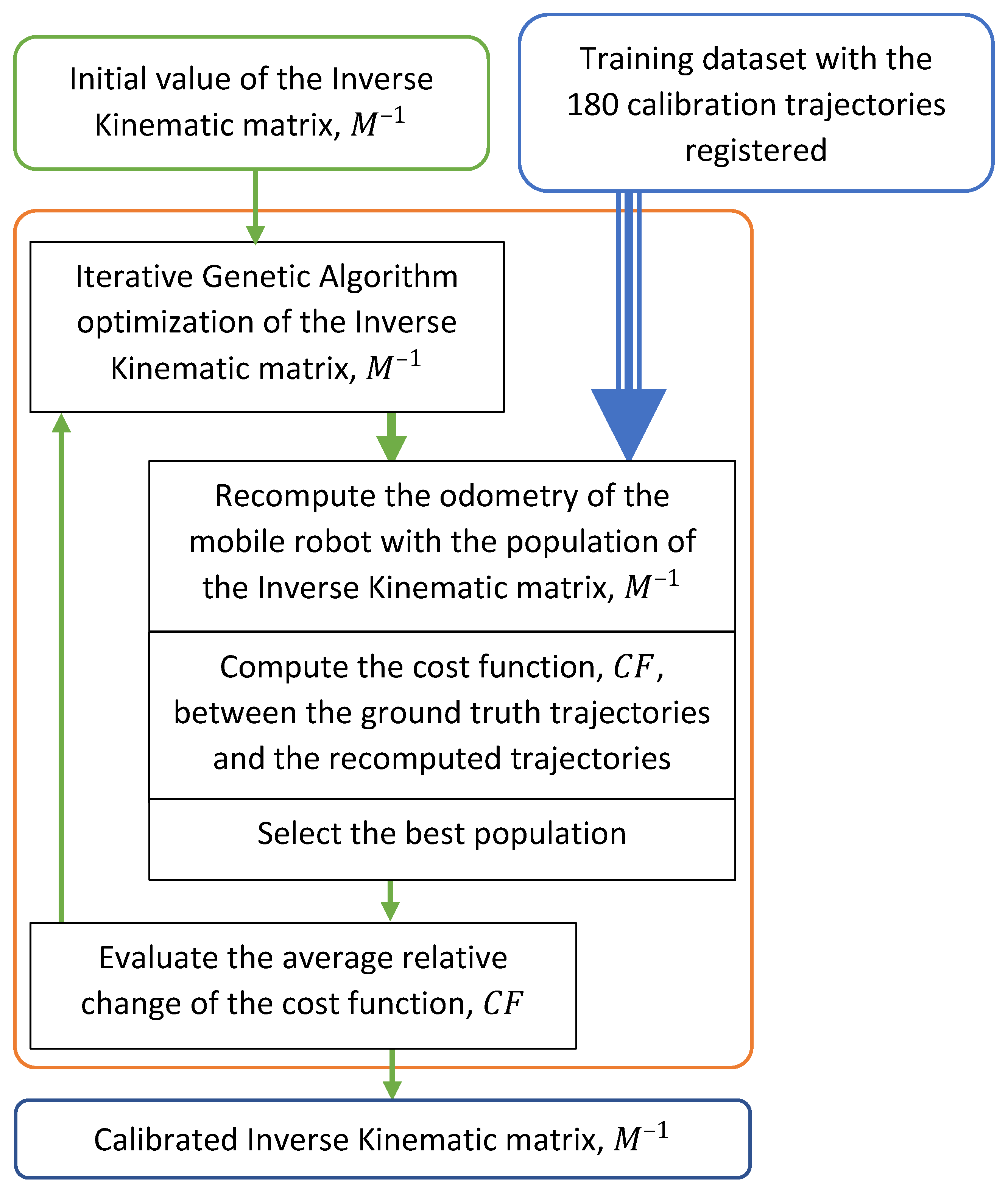
3. Procedure for Genetic Algorithm Calibration of the Inverse Kinematic Matrix

The non-parametric procedure used in this paper to calibrate the inverse kinematic matrix of the APR-02 mobile robot is based on the multivariate search capabilities of genetic algorithms [35]. This nature-inspired search is used to recompute the odometry of the mobile robot offline (Equation (1)) with the information registered while completing a trajectory. The application of a genetic search iteratively finds a local unconstrained minimum of an objective cost function in a multivariate search space. Figure 4 shows a diagram describing the genetic algorithm search, which is started from an initial population that defines a starting point in the search space and then performs a bounded search.
The initial population of the search is the theoretical value of the inverse kinematic matrix M 1 defined in Equation (3). This is interpreted by the genetic algorithm as a population vector, V , that defines the ninth-dimensional search space:
M 1 = [ m 1 , 1   m 1 , 2 m 1 , 3 m 2 , 1 m 2 , 2 m 2 , 3 m 3 , 1 m 3 , 2 m 3 , 3 ]
V = [ m 1 , 1   m 1 , 2 m 1 , 3 m 2 , 1 m 2 , 2 m 2 , 3 m 3 , 1 m 3 , 2 m 3 , 3 ]
The upper and lower bounds ( V U B and V L B ) of the GA search were configured to allow a ±10% variation of the values defined in the initial population V .
The iterative search performed by genetic algorithms requires the computation of a cost function C F to evaluate the performance of each population proposed during the search. This cost function is the same one used in [17] to compare the previous reference parametric calibration results [17] with the non-parametric calibration presented in this paper. This function is defined as:
C F = 1 Z · i = 1 Z ( x L I D A R i ( N ) x i ( F ) ) 2 + ( y L I D A R i ( N ) y i ( F ) ) 2 + ( θ L I D A R i ( N ) θ i ( F ) ) 2
where Z is the number of trajectories used to compute the cost function (the 180 trajectories included in the training dataset); i represents an individual trajectory completed by the mobile robot; x L I D A R i ( p ) is the x location of the mobile robot estimated by applying SLAM to the p scan provided by the onboard LIDAR while completing the trajectory i ; N identifies the last scan provided by the LIDAR when the robot reaches the end of the trajectory; x i ( k ) is the x location of the mobile robot estimated with the internal odometry using the current values of the inverse kinematic matrix M 1 ; F identifies the last odometry evaluation obtained when the robot reaches the end of the trajectory; θ is the final angular orientation of the mobile robot.
This cost function formulation was used to calibrate the effective kinematic parameters of an omnidirectional mobile robot by Savaee et al. [14]. This cost function apparently applies the same weights to the distance and angular error obtained at the end of the displacement. However, this perception is incorrect because an error in a specific angular orientation of the robot affects the estimation of the subsequent trajectory cumulatively (see Equation (1)). Therefore, any error in the intermediate estimation of the angular orientation has a huge potential cumulated weight in the computation of the cost function.
At this point, note that this cost function is computed using only the ending position of the mobile robot. Therefore, the evaluation of this cost function only requires: (1) the last position of the ground truth trajectory estimated with the SLAM procedure (computed while completing the trajectory) and (2) the last location estimated with the odometry using the inverse kinematic matrix defined by the current population analyzed in the iteration. This offline computation of the odometry requires all the information provided by the encoders during the displacement; this is why each trajectory registered by the mobile robot also includes the information provided by the encoders.
Finally, the iterative search performed by the genetic algorithm stops if the average relative change in the best population found of a cost function C F is less than or equal to 10−6, which is the default value used in standard GA searches.

4. Results

This section compares the performance of the inverse kinematic matrices of the APR-02 mobile robot. This section presents: (1) the reference theoretical value of the inverse kinematic matrix of the mobile robot, (2) the reference parametric calibration of the inverse kinematic matrix obtained previously in [17], and (3) the result of the non-parametric calibration performed in this paper.

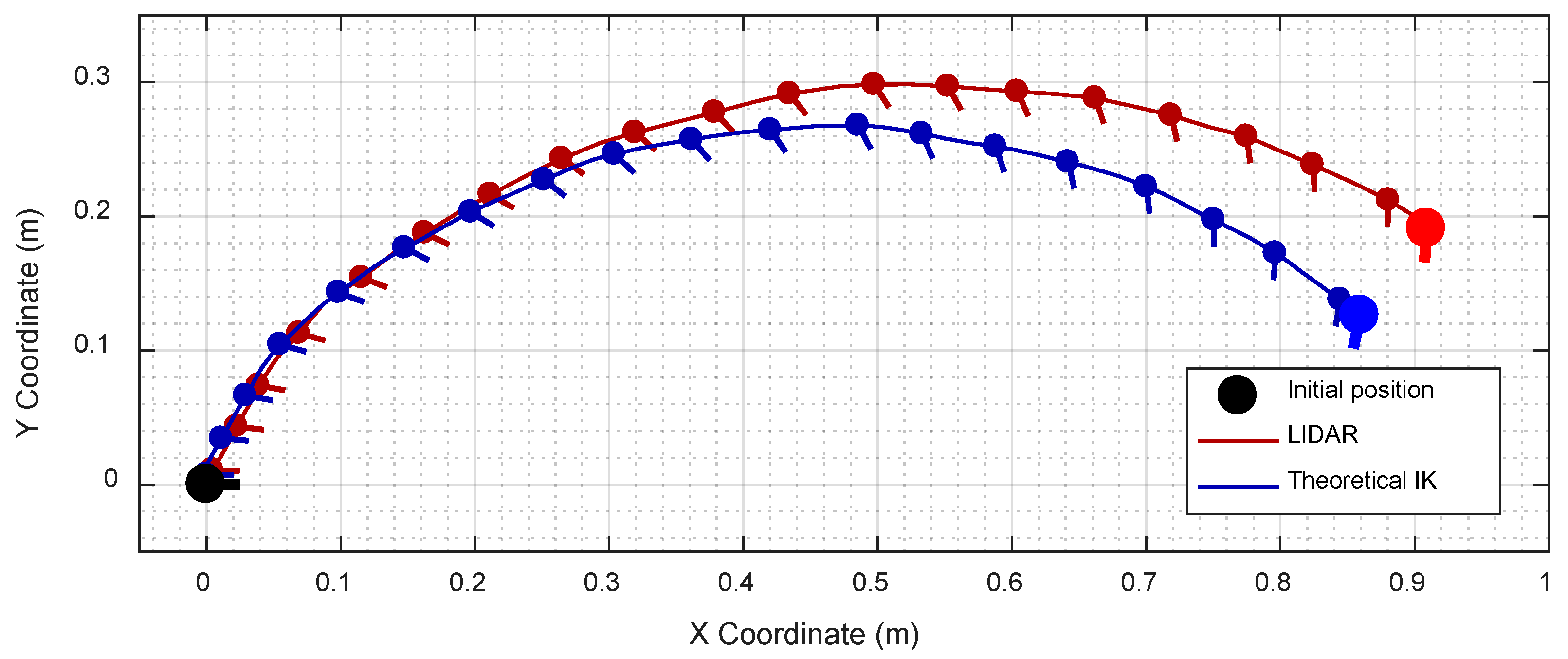
4.1. Reference Theoretical Value of the Inverse Kinematic Matrix

The exact or theoretical value of the inverse kinematic matrix ( M 1 ) of the APR-02 mobile robot can be computed analytically from Equation (1) as [17]:
M 1 = [ 0.0854478398400646             0.0000000000000000       0.0854478398400646       0.0493333333333333       0.0986666666666667       0.0493333333333333       0.2529914529914529             0.2529914529914529       0.2529914529914529 ]
Figure 5 shows the evolution of a sample trajectory followed by the APR-02 mobile robot: the red line displays the ground truth trajectory estimated with SLAM [31] and the blue line the odometry computed using the theoretical value of the inverse kinematic matrix. As could be expected, Figure 5 shows differences between the ground truth trajectory and the odometry due to the existence of systematic odometry errors. At this point, note that the inverse kinematic matrix of a three-wheeled omnidirectional robot is very sensitive to any inaccuracy in the implementation of the parameters of the motion system [17]: radii of the wheels ( r a , r b , r c ) , the distance between the center of the robot and each wheel ( R a ,   R b ,   R c ), and the angular orientation of each wheel in the mobile robot frame ( δ a ,   δ b ,   δ c ). In any case, the effects of the systematic errors are best evidenced in a mobile robot performing curved trajectories (Figure 5) rather than straight trajectories [17]. In the case of an omnidirectional mobile robot, the difference between a curved and a straight trajectory depends only on the target angular rotational speed, which is the ω parameter in the motion command, ( v , α , ω ) .

4.2. Reference Parametric Optimization of the Inverse Kinematic Matrix (from [17])

The parametric optimization presented in [17] was focused on calibrating the value of the parameters of the APR-02 mobile robot and the computation of the inverse kinematic matrix of the robot from these parameters. Nine specific mobile robot parameters were calibrated in [17]: the radii of the wheels ( r a , r b , r c ) , the distance between the center of the robot and each wheel ( R a , R b , R c ) , and the angular orientation of each wheel ( δ a , δ b , δ c ) . The computation of this parametric optimization required 903 s in a high-performance workstation.
The exact value of the inverse kinematic matrix ( M P A R A M E T R I C 1 ) obtained from the parametric calibration presented in [17] is:
M P A R A M E T R I C 1 = [ 0.0892930568372762 0.0005606566978203 0.0867466159313470       0.0520955668635434 0.1010213675626970 0.0533117820461363       0.2364093797047320       0.2341358647406650 0.2353792947863630 ]
This parametric inverse kinematic matrix represents the following errors in the determination of the parameters of the mobile robot: 4.7% in the size of the radius of the wheel a ( r a ), 2.4% in r b , 3.2% in r c , 12% in the distance from the wheel a to the center of rotation of the robot ( R a ), 10% in R b , 11% in R c , 0.4% in the angular orientation of the wheel a ( δ a ), 0.2% in δ b , and 0.5% in δ c . These huge errors obtained in the parametric calibration, higher than 10% in some cases, were too high to be justified as being caused by assembling or manufacturing errors. Therefore, the drawback of the parametric calibration was that the results could not be interpreted as an improved description of the physical parameters of the mobile robot: the radii of the wheels ( r a ,   r b ,   r c ), the distances from the wheels to the center of rotation of the mobile robot ( R a ,   R b ,   R c ), and the angular orientations of the wheels ( δ a ,   δ b ,   δ c ). Consequently, these results suggested the development of a comparative non-parametric calibration of the inverse kinematic matrix of the mobile robot.

4.3. Non-Parametic Inverse Kinematic Matrix Calibrated with Genetic Algorithms

As stated above, the difficult physical interpretation of the parametric optimization results obtained in [17] combined with the difficulty of establishing feasible limits to the parametric search suggested the implementation of an alternative non-parametric calibration of the inverse kinematic matrix of the mobile robot. The complete procedure used in this non-parametric calibration is described in Section 3. The optimization is based on the multivariate search capabilities of the genetic algorithms, which are less prone to local minima than other gradient search algorithms. The computation of this non-parametric optimization required 637 s in the same high-performance workstation used in the reference parametric optimization [17] (29% less time).
The best non-parametric inverse kinematic matrix ( M N O N P A R A M E T R I C 1 ) obtained with the application of the calibration procedure proposed in this paper (described in Section 3) is:
M N O N P A R A M E T R I C 1 = [ 0.0883286476963123       0.0000000000000000 0.0873330402667908       0.0522829495809178 0.1008246738469390 0.0536189007203205       0.2357044251338890         0.2338948216993490 0.2348793373133590 ]
The following expression is used to compare the inverse kinematic matrix obtained with the parametric (Equation (8)) and non-parametric calibration (Equation (9)). This expression performs the Hadamart product (element-wise product) [36] of the difference between these two matrices.
( M N O N P A R A M E T R I C 1 ) i j · ( 1 + M D I F F E R E N C E 1 ) i j = ( M P A R A M E T R I C 1 ) i j
M D I F F E R E N C E 1 = [             1.091 % 1.505 × 10 15 % 0.671 %     0.358 %                       0.195 % 0.572 %               0.299 %                       0.103 %         0.212 % ]
The difference matrix M D I F F E R E N C E 1 shows that the results of both calibrations (parametric and non-parametric) are very similar, with differences lower than 0.7% except in the case of the coefficients m 1 , 1 (1.091%) and m 1 , 2 ( 1.505 × 10 15 % ). The huge difference in the coefficient m 1 , 2 is because the non-parametric calibration maintained the original value defined in the theoretical inverse kinematic matrix (Equations (3) and (7)), with a value very close to zero: −1.208 × 10⁻¹⁷. Alternatively, the result of the parametric calibration performed in [17] (displayed in Equation (8)) showed m 1 , 2 to reach the value of 0.00056 , which is very difficult to interpret as a parametric inaccuracy originated during the assembling the robot. The differences between the parametric and non-parametric calibration of the inverse kinematic matrices are small but cannot be neglected because the odometry is cumulatively updated ten times per second with the displacement information provided by the encoders.
Figure 6 compares the offline computation of the odometry of four randomly chosen validation trajectories (from the 36 × 5 available in the validation dataset). The ground truth trajectory computed from the LIDAR information is labeled in red and the odometry is computed using the different inverse kinematic matrices evaluated in this paper: theoretical IK (green), parametric IK (brown), and non-parametric IK (magenta). Figure 7a–d shows in detail the final position of the robot achieved in the trajectories depicted in Figure 6. Figure 7a–d shows small differences between the ground truth trajectory of the mobile robot (red line) and the odometry computed with the parametric (brown line) and non-parametric (magenta line) inverse kinematic matrices obtained for the APR-02.
Finally, Table 2 and Table 3 compare the performance of the non-parametric calibration performed in this paper. Table 2 presents the average values of the cost function ( C F ) obtained with the 180 benchmark trajectories contained in the training dataset. The reference cost function, C F T h e o r e t i c a l   I K , was computed using the theoretical inverse kinematic matrix which is described in Equations (3) and (7). The values of the parametric inverse kinematic matrix (Parametric IK) were obtained in [17] and its values are presented in Equation (8). The numerical values of the non-parametric optimization of the inverse kinematic matrix performed in this paper with genetic algorithms (Non-parametric IK) are described in Equation (9). Table 2 shows that the best cost function computed with the training trajectories is practically the same for the parametric and non-parametric calibrations. Please note that the column indicating C F T R A I N I N G presents the cost function computed with the calibration trajectories included in the training dataset.
Table 3 shows the value of the cost function evaluated with the trajectories included in the validation dataset. These validation trajectories were registered several months after the registration of the trajectories included in the training dataset. Table 3 shows that the offline computation of the odometry of the 180 trajectories included in the validation dataset offers practically the same cost function and the same improvement with both the parametric and non-parametric inverse kinematic matrices. Additionally, the similarity between the values of the cost function obtained with the training dataset (Table 2) and the validation dataset (Table 3) seems to indicate no over-time changes in the kinematics of the mobile robot APR-02.

5. Discussion and Conclusions

This paper proposes a non-parametric calibration procedure of the effective inverse kinematic matrix of a three-wheeled omnidirectional mobile robot based on the search capabilities of genetic algorithms. The calibration procedure used a training dataset composed of five repetitions of 36 representative benchmark trajectories (180 trajectories in total). These benchmark trajectories summarize the motion performances of a three-wheeled mobile robot [17]. The calibration procedure is based on genetic algorithms because the mutation and combination performed during the search is less prone to local minima during the multivariate searches required to optimize the kinematics of a robot [14,17].
The application of this non-parametric calibration procedure to the offline computation of the odometry of the training trajectories reduced the value of the cost function from 0.1234 to 0.0215, representing an improvement of the cost function of 82.6% (see Table 2). This improvement is practically the same as that (82.6%) obtained in the parametric calibration procedure conducted previously in [17] with the same training trajectories. The analysis implemented with the validation trajectories confirmed an average improvement in the cost function of 81.8% (see Table 3) which is visually observable in the estimated trajectory of the mobile robot (see Figure 6 and Figure 7). The calibration results obtained in this paper have a similar order of magnitude as the improvements presented by Maddahi et al. [8] and Batlle et al. [23], who highlighted the importance of using curved trajectories for calibrating the kinematics of an omnidirectional mobile robot. Nevertheless, the use of different calibration trajectories precludes direct comparison of the achievements.
As a summary, the non-parametric calibration of the inverse kinematic matrix of a three-wheeled omnidirectional mobile robot has two main advantages: (1) it avoids the problem of defining feasible physical-interpretable limits applied in the parametric calibration; and (2), as a consequence, this non-parametric calibration is much easier to implement and converges faster than the parametric calibration. The offline implementation of the non-parametric calibration in a high-performance workstation required an average of 637 s, while the parametric calibration conducted previously in [17] required 903 s (41% more computational time). The definition of feasible, physically interpretable limits in a parametric calibration of the kinematic matrix is a problem that cannot be neglected because of the complex numerical relationship between the parameters that define the inverse kinematic matrix of a mobile robot. The comparative analysis of the results obtained in this paper demonstrates that the improvement in odometry that can be obtained with a non-parametric calibration is practically the same as that which can be obtained with a parametric calibration. Finally, the disadvantage of performing a non-parametric calibration of the inverse kinematic matrix of a mobile robot is that the calibration result is a numerical matrix that cannot be physically interpreted. However, this disadvantage does not really exist because the parameter variation obtained in the parametric calibration performed in [17] could not be physically interpreted either.
Future work will analyze the application of this non-parametric procedure in several three-wheeled omnidirectional mobile robots and the application of alternative methods based on artificial neural networks [37] to estimate the kinematics of an omnidirectional mobile robot.

Author Contributions

Formal analysis, E.R. and E.C.; investigation, J.P. and E.R.; methodology, J.P.; resources, R.B.; software, R.B. and E.C.; writing—original draft, E.R. and E.C.; writing—review & editing, J.P. All authors have read and agreed to the published version of the manuscript.

Funding

This research has been partially funded by the Departament de Recerca i Universitats de la Generalitat de Catalunya: FI SDUR 2022 grant.

Conflicts of Interest

The authors declare no conflict of interest. The funders had no role in the design of the study, in the collection, analyses, or interpretation of data, in the writing of the manuscript or in the decision to publish the results.

References

  1. Borenstein, J.; Feng, L. Measurement and correction of systematic odometry errors in mobile robots. IEEE Trans. Robot. Autom. 1996, 12, 869–880. [Google Scholar] [CrossRef] [Green Version]
  2. Štefek, A.; Pham, V.T.; Krivanek, V.; Pham, K.L. Optimization of Fuzzy Logic Controller Used for a Differential Drive Wheeled Mobile Robot. Appl. Sci. 2021, 11, 6023. [Google Scholar] [CrossRef]
  3. Ding, T.; Zhang, Y.; Ma, G.; Cao, Z.; Zhao, X.; Tao, B. Trajectory tracking of redundantly actuated mobile robot by MPC velocity control under steering strategy constraint. Mechatronics 2022, 84, 102779. [Google Scholar] [CrossRef]
  4. Thai, N.H.; Ly, T.T.K.; Dzung, L.Q. Trajectory tracking control for differential-drive mobile robot by a variable parameter PID controller. Int. J. Mech. Eng. Robot. Res. 2022, 11. [Google Scholar] [CrossRef]
  5. de Jesús Rubio, J.; Aquino, V.; Figueroa, M. Inverse kinematics of a mobile robot. Neural Comput. Appl. 2013, 23, 187–194. [Google Scholar] [CrossRef]
  6. Sousa, R.B.; Petry, M.R.; Moreira, A.P. Evolution of Odometry Calibration Methods for Ground Mobile Robots. In Proceedings of the IEEE International Conference on Autonomous Robot Systems and Competitions (ICARSC), Ponta Delgada, Portugal, 15–17 April 2020; pp. 294–299. [Google Scholar] [CrossRef]
  7. Hijikata, M.; Miyagusuku, R.; Ozaki, K. Wheel Arrangement of Four Omni Wheel Mobile Robot for Compactness. Appl. Sci. 2022, 12, 5798. [Google Scholar] [CrossRef]
  8. Maddahi, Y.; Maddahi, A.; Sepehri, N. Calibration of omnidirectional wheeled mobile robots: Method and experiments. Robotica 2013, 31, 969–980. [Google Scholar] [CrossRef]
  9. Lin, P.; Liu, D.; Yang, D.; Zou, Q.; Du, Y.; Cong, M. Calibration for Odometry of Omnidirectional Mobile Robots Based on Kinematic Correction. In Proceedings of the 14th International Conference on Computer Science & Education (ICCSE), Toronto, ON, Canada, 19–21 August 2019; pp. 139–144. [Google Scholar] [CrossRef]
  10. Maulana, E.; Muslim, M.A.; Hendrayawan, V. Inverse kinematic implementation of four-wheels mecanum drive mobile robot using stepper motors. In Proceedings of the 2015 International Seminar on Intelligent Technology and Its Applications (ISITIA), Surabaya, Indonesia, 20–21 May 2015; pp. 51–56. [Google Scholar] [CrossRef]
  11. Jia, Q.; Wang, M.; Liu, S.; Ge, J.; Gu, C. Research and development of mecanum-wheeled omnidirectional mobile robot implemented by multiple control methods. In Proceedings of the 2016 23rd International Conference on Mechatronics and Machine Vision in Practice (M2VIP), Nanjing, China, 28–30 November 2016; pp. 1–4. [Google Scholar] [CrossRef]
  12. Xu, H.; Yu, D.; Wang, Q.; Qi, P.; Lu, G. Current Research Status of Omnidirectional Mobile Robots with Four Mecanum Wheels Tracking based on Sliding Mode Control. In Proceedings of the 2019 IEEE International Conference on Unmanned Systems and Artificial Intelligence (ICUSAI), Xi’an, China, 22–24 November 2019; pp. 13–18. [Google Scholar] [CrossRef]
  13. Li, Y.; Ge, S.; Dai, S.; Zhao, L.; Yan, X.; Zheng, Y.; Shi, Y. Kinematic Modeling of a Combined System of Multiple Mecanum-Wheeled Robots with Velocity Compensation. Sensors 2020, 20, 75. [Google Scholar] [CrossRef] [Green Version]
  14. Savaee, E.; Hanzaki, A.R. A New Algorithm for Calibration of an Omni-Directional Wheeled Mobile Robot Based on Effective Kinematic Parameters Estimation. J. Intell. Robot. Syst. 2021, 101, 28. [Google Scholar] [CrossRef]
  15. Bożek, A. Discovering Stick-Slip-Resistant Servo Control Algorithm Using Genetic Programming. Sensors 2022, 22, 383. [Google Scholar] [CrossRef]
  16. Prados Sesmero, C.; Buonocore, L.R.; Di Castro, M. Omnidirectional Robotic Platform for Surveillance of Particle Accelerator Environments with Limited Space Areas. Appl. Sci. 2021, 11, 6631. [Google Scholar] [CrossRef]
  17. Palacín, J.; Rubies, E.; Clotet, E. Systematic Odometry Error Evaluation and Correction in a Human-Sized Three-Wheeled Omnidirectional Mobile Robot Using Flower-Shaped Calibration Trajectories. Appl. Sci. 2022, 12, 2606. [Google Scholar] [CrossRef]
  18. Sharma, H.P.; Pant, M.; Agarwal, R.; Karatangi, S.V. Self-directed Robot for Car Driving Using Genetic Algorithm. In Technology Innovation in Mechanical Engineering. Lecture Notes in Mechanical Engineering; Chaurasiya, P.K., Singh, A., Verma, T.N., Rajak, U., Eds.; Springer: Singapore, 2022. [Google Scholar] [CrossRef]
  19. Tagliani, F.L.; Pellegrini, N.; Aggogeri, F. Machine Learning Sequential Methodology for Robot Inverse Kinematic Modelling. Appl. Sci. 2022, 12, 9417. [Google Scholar] [CrossRef]
  20. Zhu, Z.; Liu, Y.; He, Y.; Wu, W.; Wang, H.; Huang, C.; Ye, B. Fuzzy PID Control of the Three-Degree-of-Freedom Parallel Mechanism Based on Genetic Algorithm. Appl. Sci. 2022, 12, 11128. [Google Scholar] [CrossRef]
  21. Cardoza Plata, J.E.; Olguín Carbajal, M.; Herrera Lozada, J.C.; Sandoval Gutierrez, J.; Rivera Zarate, I.; Serrano Talamantes, J.F. Simulation and Implementation of a Mobile Robot Trajectory Planning Solution by Using a Genetic Micro-Algorithm. Appl. Sci. 2022, 12, 11284. [Google Scholar] [CrossRef]
  22. Rahmaniar, W.; Rakhmania, A. Mobile Robot Path Planning in a Trajectory with Multiple Obstacles Using Genetic Algorithms. J. Robot. Control. 2021, 3, 1–7. [Google Scholar] [CrossRef]
  23. Batlle, J.A.; Font-Llagunes, J.M.; Barjau, A. Calibration for mobile robots with an invariant Jacobian, Robot. Auton. Syst. 2010, 58, 10–15. [Google Scholar] [CrossRef]
  24. Clotet, E.; Martínez, D.; Moreno, J.; Tresanchez, M.; Palacín, J. Assistant Personal Robot (APR): Conception and Application of a Tele-Operated Assisted Living Robot. Sensors 2016, 16, 610. [Google Scholar] [CrossRef] [Green Version]
  25. Palacín, J.; Clotet, E.; Martínez, D.; Martínez, D.; Moreno, J. Extending the Application of an Assistant Personal Robot as a Walk-Helper Tool. Robotics 2019, 8, 27. [Google Scholar] [CrossRef] [Green Version]
  26. Palacín, J.; Martínez, D.; Clotet, E.; Pallejà, T.; Burgués, J.; Fonollosa, J.; Pardo, A.; Marco, S. Application of an Array of Metal-Oxide Semiconductor Gas Sensors in an Assistant Personal Robot for Early Gas Leak Detection. Sensors 2019, 19, 1957. [Google Scholar] [CrossRef] [Green Version]
  27. Penteridis, L.; D’Onofrio, G.; Sancarlo, D.; Giuliani, F.; Ricciardi, F.; Cavallo, F.; Greco, A.; Trochidis, I.; Gkiokas, A. Robotic and Sensor Technologies for Mobility in Older People. Rejuvenation Res. 2017, 20, 401–410. [Google Scholar] [CrossRef] [PubMed] [Green Version]
  28. Palacín, J.; Martínez, D.; Rubies, E.; Clotet, E. Suboptimal Omnidirectional Wheel Design and Implementation. Sensors 2021, 21, 865. [Google Scholar] [CrossRef]
  29. Bitriá, R.; Palacín, J. Optimal PID Control of a Brushed DC Motor with an Embedded Low-Cost Magnetic Quadrature Encoder for Improved Step Overshoot and Undershoot Responses in a Mobile Robot Application. Sensors 2022, 22, 7817. [Google Scholar] [CrossRef]
  30. Palacín, J.; Rubies, E.; Clotet, E.; Martínez, D. Evaluation of the Path-Tracking Accuracy of a Three-Wheeled Omnidirectional Mobile Robot Designed as a Personal Assistant. Sensors 2021, 21, 7216. [Google Scholar] [CrossRef]
  31. Lluvia, I.; Lazkano, E.; Ansuategi, A. Active Mapping and Robot Exploration: A Survey. Sensors 2021, 21, 2445. [Google Scholar] [CrossRef] [PubMed]
  32. Palacín, J.; Martínez, D.; Rubies, E.; Clotet, E. Mobile Robot Self-Localization with 2D Push-Broom LIDAR in a 2D Map. Sensors 2020, 20, 2500. [Google Scholar] [CrossRef] [PubMed]
  33. Popovici, A.-T.; Dosoftei, C.-C.; Budaciu, C. Kinematics Calibration and Validation Approach Using Indoor Positioning System for an Omnidirectional Mobile Robot. Sensors 2022, 22, 8590. [Google Scholar] [CrossRef]
  34. Mora, A.; Prados, A.; Mendez, A.; Barber, R.; Garrido, S. Sensor Fusion for Social Navigation on a Mobile Robot Based on Fast Marching Square and Gaussian Mixture Model. Sensors 2022, 22, 8728. [Google Scholar] [CrossRef]
  35. Fraser, A. Simulation of genetic systems by automatic digital computers. I. Introduction. Aust. J. Biol. Sci. 1957, 10, 484–491. [Google Scholar] [CrossRef] [Green Version]
  36. George, P.H. Styan, Hadamard products and multivariate statistical analysis. Linear Algebra Its Appl. 1973, 6, 217–240. [Google Scholar] [CrossRef] [Green Version]
  37. Boanta, C.; Brișan, C. Estimation of the Kinematics and Workspace of a Robot Using Artificial Neural Networks. Sensors 2022, 22, 8356. [Google Scholar] [CrossRef] [PubMed]
Figure 1. APR-02 mobile robot performing a transversal (or lateral) displacement: (a) starting point; (b,c) intermediate points; and (d) destination point.
Applsci 13 01053 g001
Figure 2. Detail of the omnidirectional motion system of the APR-02 mobile robot. ( X R , Y R ) is the mobile robot frame in which X R represents the front and forward direction of the robot.
Applsci 13 01053 g002
Figure 3. Parametric definition of the omnidirectional motion system of the APR-02 mobile robot. ( X R , Y R ) represents the mobile robot frame in which X R is the front of the mobile robot.
Applsci 13 01053 g003
Figure 4. Diagram of the Genetic Algorithm search performed to calibrate the inverse kinematic matrix of the APR-02 mobile robot.
Applsci 13 01053 g004
Figure 5. Sample trajectory followed by the APR-02 mobile robot for the motion command ( v , α , ω 0 ) = (0.2 m/s, 30°, 0.35 rad/s). The ground truth trajectory was estimated from the information of the LIDAR (red line) while the odometry was estimated with the theoretical value of the inverse kinematic matrix of the mobile robot (blue line).
Applsci 13 01053 g005
Figure 6. Comparison between the ground truth trajectory followed by the mobile robot (red line) and the odometry estimated with: the theoretical IK (green line), the parametric IK (brown line) and the non-parametric IK (magenta line). Trajectories originated by the following motion commands, ( v , α , ω ) : (a) (0.2 m/s, 30°, 0.35 rad/s); (b) (0.2 m/s, 210°, 0.35 rad/s); (c) (0.2 m/s, 120°, 0.35 rad/s); and (d) (0.2 m/s, 300°, 0.35 rad/s).
Applsci 13 01053 g006
Figure 7. Detail of the final position of the robot corresponding to the full trajectories displayed in Figure 6. Ground truth trajectory of the mobile robot (red) and odometry of the mobile robot computed using the theoretical IK (green), the parametric IK [17] (brown) and the noon-parametric IK (magenta).
Applsci 13 01053 g007
Table 1. Information registered by the mobile robot while performing a calibration trajectory.
ParameterDescription
( v , α , ω , d ) Target motion command for the robot
v : translational velocity of the displacement of the robot, (m/s)
α : angular orientation of the displacement, (°)
ω : angular rotational speed of the robot during the displacement, (rad/s)
d : linear distance to be achieved during the displacement, (m)
( ω M a , ω M b , ω M c ) Target angular velocities for the wheels
ω M i : target angular velocity defined for the motor of the wheel i , computed when receiving the motion command, (rpm)
ω a , b , c = [ t ( k = 1 F ) ω a ( k = 1 F ) ω b ( k = 1 F ) ω c ( k = 1 F ) ] Angular velocities of the wheels provided by the encoders
t ( k ) : time the update k was received, (s)
ω i : instantaneous angular velocity measured by the encoder of the motor i , updated periodically at a frame rate of 10 ms, (rpm)
( x , y , θ ) = [ x ( k = 1 F ) y ( k = 1 F ) θ ( k = 1 F ) ] Trajectory of the mobile robot estimated with the odometry
x , y : location of the robot, (m)
θ : angular orientation of the robot, (°)
L I D A R = [ t L I D A R ( p = 1 ) t L I D A R ( p = N ) [ d ( 1 ) d ( 1080 ) ] 1 [ d ( 1 ) d ( 1080 ) ] N ] Scans provided by the onboard LIDAR
t L I D A R ( p ) : time the scan p was received, (s)
d ( r ) : distance scan corresponding to the angular orientation r , updated periodically at a frame rate from 200 to 300 ms, (mm)
( x , y , θ ) L I D A R = [ x L I D A R ( p = 1 N ) y L I D A R ( p = 1 N ) θ L I D A R ( p = 1 N ) ] Ground Truth trajectory of the mobile robot estimated with SLAM
x L I D A R , y L I D A R : location of the robot, (m)
θ L I D A R : angular orientation of the robot, (°)
Table 2. Values of the cost function obtained when computing the odometry of the 180 trajectories included in the training dataset with the theoretical and calibrated inverse kinematic matrices.
M 1 C F T h e o r e t i c a l   I K C F T R A I N I N G Improvement
Theoretical IK0.1234--
Parametric IK [17]0.12340.021582.61%
Non-parametric IK *0.12340.0215 *82.60% *
* Calibration result obtained in this paper.
Table 3. Values of the cost function obtained when computing the odometry of the 180 trajectories included in the validation dataset with the theoretical and calibrated inverse kinematic matrices.
M 1 C F T h e o r e t i c a l   I K C F V A L I D A T I O N Improvement
Theoretical IK0.1251--
Parametric IK [17]0.12510.022981.68%
Non-parametric IK *0.12510.0227 *81.81% *
* Calibration result obtained in this paper.
Disclaimer/Publisher’s Note: The statements, opinions and data contained in all publications are solely those of the individual author(s) and contributor(s) and not of MDPI and/or the editor(s). MDPI and/or the editor(s) disclaim responsibility for any injury to people or property resulting from any ideas, methods, instructions or products referred to in the content.

