Three-Dimensional Rendezvous Controls of Multiple Robots with Amplitude-Only Measurements in Cluttered Underwater Environments

Abstract

This study addresses multi-robot distributed rendezvous controls in cluttered underwater environments with many unknown obstacles. In underwater environments, a Unmanned Underwater Vehicle (UUV) cannot localize itself, since a Global Positioning System (GPS) is not available. Assume that each UUV has multiple signal intensity sensors surrounding it. Multiple intensity sensors on a UUV can only measure the amplitude of signals generated from its neighbor UUVs. We prove that multiple UUVs with bounded speed converge to a designated rendezvous point, while maintaining the connectivity of the communication network. This study further discusses a fault detection method, which detects faulty UUVs based on local sensing measurements. In addition, the proposed rendezvous control is adaptive to communication link failure or invisible UUVs. Note that communication link failure or invisible UUVs can happen due to unknown obstacles in the workspace. As far as we know, our study is novel in developing 3D coordinate-free distributed rendezvous control, considering underwater robots that can only measure the amplitude of signals emitted from neighboring robots. The proposed rendezvous algorithms are provably complete, and the effectiveness of the proposed rendezvous algorithms is demonstrated under MATLAB simulations.

1. Introduction

Networked robots have various applications, such as monitoring large environments, rescue missions, and target chasing [1,2,3,4]. Multiple coordinated robots are also used to perform many specific tasks, such as rendezvous [5,6,7], spacecraft docking [8], environmental monitoring [9,10,11], underwater target chasing [12], and formation control [13,14,15].

This study addresses multi-robot rendezvous controls in cluttered underwater environments with many unknown obstacles. Unmanned Underwater Vehicles (UUVs) can be divided into two categories based on whether their bodies are streamlined. The UUV’s shape is determined by the requirements of the application. For example, a streamlined shape reduces water resistance and is preferable if the UUV is required to move at high speeds. However, if underwater detection or operation tasks are the primary roles of a UUV, a non-streamlined shape is often preferred.

Because of the good water pressure resistance of spherical objects, spherical UUVs can perform rotational motions with a 0 degree turn radius. In the literature, various spherical UUVs have been developed [16,17,18,19,20]. References [16,18,19,20,21] addressed a spherical UUV with hybrid propulsion devices including vectored water jet and propeller thrusters. The three Degree-of-Freedom (DoF) motions, including surging, heaving, and yawing, were performed in a swimming pool. References [16,19,21] further demonstrated that by adopting vectored water jets, a spherical UUV can be made to maneuver freely in any direction. Considering a spherical UUV, [22] used fuzzy proportional–integral–derivative (PID) controllers to independently control the robot’s movement in all directions. Since spherical UUVs are highly maneuverable, our study considers a spherical UUV [16,17,18,19,20] as our platform.

We address practical application scenarios where multi-robot rendezvous controls are used. Recently, several studies [23,24,25] handled distributed formation control of multiple robots in environments with obstacles. For instance, a group of robots can be used for tracking a target while measuring the target’s signal [26]. During the robots’ maneuvering in formation controls, robots need to preserve the network connectivity. In order to make all robots gather close to each other, distributed rendezvous controls can be applied occasionally. In other words, distributed rendezvous algorithms can be used as a multi-robot control module to allow a team of robots to maintain network connectivity while they maneuver. For example, we can run rendezvous controls occasionally, so that all robots get closer to a root robot which leads the formation. Moreover, all robots need to get closer to the root robot, in the case where they move through a narrow tunnel.

Furthermore, rendezvous algorithms can be utilized in multi-robot collection or charging scenarios [27]. Suppose that there is a charging station close to a robot, called the root. All the robots can be charged from the charging station, once they gather close to the root.

The difficulty of the rendezvous problem decreases when a robot is equipped with Global Positioning Systems (GPS). However, GPS is unavailable in underwater environments. In difficult scenarios without GPS, robots cannot move toward a designated rendezvous point directly. Thus, we introduce a distributed rendezvous approach that does not require global localization.

A rendezvous algorithm is considered distributed, when it depends on the local interaction between neighboring robots. A distributed rendezvous algorithm is practical, since a robot cannot communicate with another robot that is too far away. Furthermore, obstacles in cluttered 3D environments can easily block the communication links between robots. In this study, we propose distributed rendezvous algorithms for UUVs in 3D unknown environments with many obstacles. Here, unknown obstacles can lead to communication link failure or invisible robots. The proposed rendezvous control is adaptive to communication link failure or invisible robots.

Considering 3D underwater environments, this study addresses the problem of enabling a network of UUVs to rendezvous at a designated root robot. Any robot in the network can be set as the root robot. Thus, the rendezvous system in this study is referred to as the any-robot rendezvous system.

The rendezvous controls in this study consider a UUV that can only measure the signal intensity emitted from its neighbor UUV. Thus, the proposed rendezvous control is suitable for a cheap UUV, which only has sensors for measuring the signal strength.

Reference [28] addressed a received signal strength (RSS) sensor model for underwater sound propagation. We consider multiple UUVs such that each UUV has multiple signal intensity sensors surrounding it. Each intensity sensor can measure the RSS of sound generated from a neighbor UUV [28].

Multiple intensity sensors on a UUV can only measure the amplitude (intensity) of signals emitted from its neighboring UUVs. To enable a distributed rendezvous based on amplitude-only measurements, we utilize a method of making a UUV approach the source of the signal (neighbor UUV) by measuring the intensity of signal at multiple intensity sensors.

We demonstrate that our distributed rendezvous algorithms are provably complete in achieving multi-robot rendezvous in cluttered 3D environments. The proposed 3D rendezvous controls assure the convergence to a designated UUV, while maintaining the connectivity of the time-varying and position-dependent communication network.

Moreover, the proposed rendezvous controls can handle the case where some UUVs are broken. While controlling the networked system, any UUV, including the root UUV, can become faulty owing to various reasons, such as hardware malfunction. This study, thus, discusses a fault detection method, which detects faulty UUVs based on local sensing measurements. Once a UUV failure is sensed, then we update the network structure, so that healthy UUVs without faults can be controlled effectively.

This study handles scenarios where multiple UUVs are deployed in cluttered 3D environments (e.g., [29]). In obstacle-rich environments, the communication (interaction) link between UUVs may be easily blocked owing to obstacles. Furthermore, invisible UUVs may occur, since line-of-sight can be blocked by unknown obstacles. In such scenarios, it is important to assure that the communication link is preserved, while every UUV maneuvers. The proposed distributed rendezvous control is unique in overcoming communication link failure or invisible UUVs. Note that communication link failure or invisible UUVs may happen due to unknown obstacles in cluttered 3D environments.

We address a distributed rendezvous control for spherical UUVs with bounded speed, such that each UUV can only measure the strength of signals emitted from neighboring UUVs. The contributions of our study are summarized as follows.

• As far as we know, this study is novel in developing 3D distributed rendezvous controls, considering a UUV that can only measure the strength of signals emitted from neighboring UUVs.
• The proposed 3D rendezvous controls are provably complete, since we prove the rendezvous to the root UUV, while maintaining the connectivity of the time-varying and position-dependent communication network.
• To the best of our knowledge, our study is unique in addressing a fault detection method that detects faulty UUVs based on local sensing measurements. In addition, the proposed rendezvous controls are adaptive to communication link failure or invisible UUVs.

The study is organized as follows. Section 2 provides the literature review of this study. Section 3 provides the background information of this study. Section 4 discusses the 3D distributed rendezvous controls introduced in this study. Section 5 provides the simulation results of this study. Section 6 provides the conclusions of this study.

2. Literature Review

Considering 2D environments, there are many studies on distributed controllers to make all robots rendezvous, considering the case where a robot measures the relative position of its nearby robot [7,30,31,32]. In [33], circumcenter-based consensus algorithms were introduced to achieve distributed rendezvous of multiple robots. However, how to handle faulty robots was not discussed in [33]. Considering 2D environments, [34] introduced rendezvous controllers that are tolerant to faulty robots. However, this method needs a controllable sensing range, which may not be feasible in practice. The authors of [35] considered the optimal consensus problem of asynchronous sampling single-integrator and double-integrator multi-robot systems utilizing distributed model predictive control algorithms.

Event-driven rendezvous strategies [36,37,38] for multi-agent systems were motivated by the use of embedded microprocessors with limited resources that will gather information and actuate the individual agent controller updates. Considering event-triggered rendezvous controls, [38] proved that if the communication graph is connected, consensus is achieved exponentially. The authors of [37] showed that with appropriate control gains in event-triggering conditions, subsystems employing discrete-time signals from neighbors achieve the state consensus. The authors of [36] studied the rendezvous problem of multi-robot systems by parallel event-triggered connectivity-preserving controls. The event-triggered control laws in [36] can assure the system convergence, and can maintain the connectivity of the time-varying and position-dependent communication network. However, [36,37,38] considered 2D environments without obstacles. In cluttered underwater environments, obstacles can block the communication link between robots, resulting in the loss of a robot.

Our study handles practical scenarios where multiple underwater robots are deployed in cluttered environments (e.g., [29]). In obstacle-rich environments, the communication (interaction) link between robots may be blocked owing to obstacles. In such scenarios, it is important to assure that the communication link is preserved while every robot maneuvers. As far as we know, the proposed distributed rendezvous control is unique in overcoming communication link failure or invisible robots.

As far as we know, other studies on distributed rendezvous controls [7,30,31,32,36,37,38] assumed that a robot can measure the relative position of its neighbor robot using local sensors, such as laser. However, no physical sensors were clearly described for this local interaction. In other words, other rendezvous controls in [7,30,31,32,36,37,38] were designed, while the specific sensors that were used for the controls were not considered. However, considering specific sensors is crucial, since robots move based on local sensing measurements.

Considering 2D environments, [39] addressed rendezvous algorithms using received signal strength indicator (RSSI) data from the radio. Reference [40] addressed a simple rendezvous algorithm using RSSI data from the radio. Reference [40] used a small, low-cost, modular robotics platform in 2D environments. Reference [40] explored the potential for using RSSI in platforms equipped with radios in order to rendezvous at a desired location or agent. The authors of [39] addressed multi-robot rendezvous with range-only measurements. However, references [39,40] considered simple 2D environments with no obstacles. In addition, [39,40] did not show that their rendezvous algorithm is provably complete in achieving multi-robot rendezvous. Moreover, [39,40] did not consider how to handle the case where a UUV is broken.

In [41], the authors applied radars with a variable sensing range in order to make all robots rendezvous in 3D environments. However, obstacle environments were not considered in [41]. Unknown obstacles can block the communication link between robots in practice. Moreover, in underwater environments, electromagnetic signals easily dissipate, and thus, radars are not suitable in underwater environments.

In 3D underwater environments, a UUV needs to be equipped with expensive 3D sonar sensors with sensing arrays, in order to measure the relative position of its neighbor UUV. However, the intensity sampling sensors used in our study are not sufficient for measuring the relative position of a neighbor UUV. In other words, intensity sensors used in our study cannot be used for measuring the relative position of a neighbor UUV.

To the best of our knowledge, our study is novel in developing provably complete 3D distributed rendezvous controls, considering a UUV which can only measure the strength of signals emitted from neighboring UUVs. Moreover, our study is unique in introducing a 3D rendezvous control, which is robust to intensity sensor failures or UUV failures.

3. Background Information

3.1. Reference Frames

Two reference frames are used in our study: an inertial reference frame $\left\{I\right\}$ and a body−fixed frame $\left\{B\right\}$ [42]. The origin of $\left\{I\right\}$ is an appropriate position with three axes pointing north, east, and down, respectively. The body−fixed frame $\left\{B\right\}$ is fixed to a UUV’s body and acts as the moving frame. The origin of $\left\{B\right\}$ is fixed at the UUV’s center.

Let $\varphi ,\theta ,\psi$ present the euler roll, euler pitch, and euler yaw, respectively. The counterclockwise (CC) rotation of $\psi$ centered at the z-axis in $\left\{B\right\}$ is as follows:

$$\begin{array}{c}\hfill \mathbf{R}\left(\psi \right)=\left(\begin{array}{ccc}cos\left(\psi \right)& -sin\left(\psi \right)& 0\\ sin\left(\psi \right)& cos\left(\psi \right)& 0\\ 0& 0& 1\end{array}\right).\end{array}$$

(1)

The CC rotation of $\theta$ centered at the y-axis in $\left\{B\right\}$ is as follows:

$$\begin{array}{c}\hfill \mathbf{R}\left(\theta \right)=\left(\begin{array}{ccc}cos\left(\theta \right)& 0& sin\left(\theta \right)\\ 0& 1& 0\\ -sin\left(\theta \right)& 0& cos\left(\theta \right)\end{array}\right).\end{array}$$

(2)

The CC rotation of $\varphi$ centered at the x-axis in $\left\{B\right\}$ is as follows:

$$\begin{array}{c}\hfill \mathbf{R}\left(\varphi \right)=\left(\begin{array}{ccc}1& 0& 0\\ 0& cos\left(\varphi \right)& -sin\left(\varphi \right)\\ 0& sin\left(\varphi \right)& cos\left(\varphi \right)\end{array}\right).\end{array}$$

(3)

The combined rotation matrix is built by multiplying the yaw, pitch, and roll rotation matrices in this order to obtain the following:

$$\begin{array}{c}\hfill \mathbf{R}(\psi ,\theta ,\varphi )=\mathbf{R}\left(\psi \right)\mathbf{R}\left(\theta \right)\mathbf{R}\left(\varphi \right).\end{array}$$

(4)

Figure 1 depicts three euler angles ($\varphi$, $\theta$, and $\psi$). In this figure, there is a spherical UUV, and we plot a cross-shaped propeller at the back of the UUV. Furthermore, this figure depicts the inertial reference frame $\left\{I\right\}$ and the body−fixed frame $\left\{B\right\}$.

3.2. Graph Theory

We present several definitions from graph theory in [43]. First, $G=\left(V\right(G),E(G\left)\right)$ is an undirected graph with a vertex set V and an edge set E. The two vertices at the end of an edge e are called neighbors.

A tree (T) is a connected graph containing no cycles. Thus, a path connecting any two vertices in a tree T is unique. One vertex of T is set as the root. In T, $p\left(v\right)$, the parent of v, is the neighbor of v along the path to the root. Furthermore, $c\left(v\right)$, the child of v, is a vertex such that v is the parent of $c\left(v\right)$. A leaf is a vertex with no children. A descendant of v is a vertex that is either $c\left(v\right)$ or is the descendant of $c\left(v\right)$ (recursively). An ancestor of v is a vertex that is either $p\left(v\right)$ or is the ancestor of $p\left(v\right)$ (recursively). Figure 2 depicts a tree T.

3.3. Assumptions and Definitions

This subsection discusses the assumptions and definitions used in this study. Suppose we have N UUVs in total. Let $u_i$ indicate the i-th UUV ($i\in \{1,2,\dots ,N\}$). Let $u_N$ indicate the root in the robot network. In our study, $u_N$ is set as the root of a tree graph T. In the inertial reference frame, ${\mathbf{u}}_i\in {\mathbb{R}}^3$ is the 3D location of a UUV $u_i$.

A UUV has communication devices to enable information sharing with its neighboring UUVs. This local communication ability is fundamental for multi-agent controls as well as for handling UUV faults.

Consider a UUV that has six signal intensity sensors surrounding it. Each intensity sensor can measure the received signal strength of sound generated from a neighbor UUV [28]. As a UUV, e.g., $u_i$, detects a signal from its neighbor UUV $u_j$, six intensity sensors on $u_i$ can measure the strength of the signal emitted from $u_j$.

Figure 3 plots the local coordinates of every intensity sensors positioned on a UUV. The local coordinates are defined in the UUV’s body−fixed frame. In Figure 3, the path of signal emitted from the emitter is illustrated with dotted arrow. The origin of the local coordinates frame is at the UUV’s center. The numbering in front of local coordinates indicates the index of the associated intensity sensor. For instance, $1:[dr,0,0]$ indicates that the first sensor has local coordinates $[dr,0,0]$. We can see that every intensity sensor is positioned at an equidistant point from the UUV’s center. Here, $dr$ is the relative distance between the UUV’s center and any other sensor.

In the body−fixed frame of $u_i$, let ${\mathbf{c}}_i^r\in {\mathbb{R}}^3$ indicate the local coordinates of the r-th intensity sensor ($r\in \{1,2,\dots ,6\}$) of $u_i$. Let $P\left({\mathbf{c}}_i^r\right)\in \mathbb{R}$ indicate the signal power received by the r-th intensity sensor ($r\in \{1,2,\dots ,6\}$) of $u_i$. Recall that Figure 3 plots the local coordinates of every intensity sensor positioned on $u_i$.

In emitter localization, complexity increases owing to obstacles blocking the line-of-sight (LOS) path between an intensity sensor and an emitter [44,45,46,47,48,49]. Considering an LOS emitter, the Received Signal Strength Indicator (RSSI) is modeled utilizing a log-normal shadowing model [28,50]. Based on the log-normal shadowing model in [28], we use the following equation:

$$\begin{array}{c}\hfill P\left({\mathbf{c}}_i^r\right)=P_0-10E_{p}lo{g}_{10}\left(d_I\right)+\gamma (d_I-1)+n^P.\end{array}$$

(5)

where $d_I$ indicates the relative distance between the intensity sensor at the local coordinates ${\mathbf{c}}_i^r\in {\mathbb{R}}^3$ and the emitter, $P_0$ (dB) is the received signal power at 1 m, $E_p$ is the propagation exponent, and $n^P$ is a random variable with mean 0 and standard deviation ${\sigma }^P$.

In Equation (5), $\gamma$ is the path loss exponent (PLE), which models the geometric spreading loss. The term $\gamma$ (dB/m) is the frequency-dependent medium absorption, and $\gamma$ can be determined using Thorp’s model, which is based on the experiments in [28].

We consider the case where all sensors of a UUV are identical to those of another UUV. Let $P\left(u_i\right)\in \mathbb{R}$ denote the average intensity measurement associated with $u_i$. We have

$$\begin{array}{c}\hfill P\left(u_i\right)=\frac{1}{6}\sum _{r=1}^{6}P\left({\mathbf{c}}_i^r\right).\end{array}$$

(6)

It is assumed that $P_0$, $E_p$, and ${\sigma }^P$ in Equation (5) are known a priori. This is feasible using experiments with UUVs [28]. For realistic simulations of the RSSI for an underwater emitter, we use the model parameters in [28]. In Equation (5), $P_0$ = 100 dB, $E_p=2$, $\gamma =0.05$, ${\sigma }^P=1$ are used, according to [28]. In this case, Figure 4 shows the relationship between $d_I$ and $P\left(u_i\right)$ using (5) and (6). As $d_I$ increases, $P\left(u_i\right)$ decreases.

It is assumed that if $P\left(u_i\right)>P_{thres}$, then SNR is sufficiently large and the intensity sensor can detect the LOS signal generated from the emitter. We say that a UUV $u_i$ is a neighbor to UUV $u_j$ if $P\left(u_i\right)>P_{thres}$ and $P\left(u_j\right)>P_{thres}$. Here, $P_{thres}$ is a tuning parameter for determining a neighbor.

The neighbor information can be set by mutual communication between $u_i$ and $u_j$. In the case where $u_i$ and $u_j$ are neighbors, $\parallel {\mathbf{u}}_i-{\mathbf{u}}_j\parallel <r_s\left(P_{thres}\right)$ and the LOS between $u_i$ and $u_j$ is not blocked by obstacles. Here, $r_s\left(P_{thres}\right)$ can be considered as the maximum sensing range for a UUV. Note that $r_s\left(P_{thres}\right)$ is determined by $P_{thres}$. As $P_{thres}$ decreases, $r_s\left(P_{thres}\right)$ increases using (5).

For notation convenience, we use $r_s$ instead of $r_s\left(P_{thres}\right)$. See Figure 4 for an illustration. If we set $P_{thres}=52$ dB, then $r_s=10$ m; if we set $P_{thres}=20$ dB, then $r_s=60$ m.

We say that a UUV $u_i$ encounters $u_j$ if $\parallel {\mathbf{u}}_i-{\mathbf{u}}_j\parallel <ϵ\approx 0$. Let $P^e$ denote the signal power measured when $u_i$ encounters $u_j$. Thus, using Equation (5), we obtain the following:

$$\begin{array}{c}\hfill P^e=P_0-10E_{p}lo{g}_{10}\left(ϵ\right)+\gamma (ϵ-1).\end{array}$$

(7)

If both $P\left(u_i\right)$ and $P\left(u_j\right)$ exceed $P^e$, then we assume that $u_i$ encountered $u_j$.

Let $G=\left(V\right(G),E(G\left)\right)$ indicate the graph presenting the networked system. Every node in $V\left(G\right)$ indicates a UUV. An edge, e.g., $\{u_i,u_j\}\in E\left(G\right)$, indicates that $u_i$ and $u_j$ are neighboring UUVs. Recall that $u_i$ is a neighbor to $u_j$ if $P\left(u_i\right)>P_{thres}$ and $P\left(u_j\right)>P_{thres}$. Since we check both $P\left(u_i\right)$ and $P\left(u_j\right)$ for detecting neighbors, G is an undirected graph.

Let $G_0=(V_0,E_0)$ indicate the initial connectivity network (at sampling step $t=0$). Without loss of generality, it is assumed that $G_0$ is connected. As far as we know, this initial connectivity assumption is required for any distributed rendezvous controls in the literature [34,41,51,52]. This is due to the fact that distributed rendezvous controls are based on local interaction between neighboring agents.

Note that the initial connectivity assumption does not assure that the network connectivity is maintained during the maneuver of an agent. As agents move around, the communication link among them may be broken due to obstacles in the environments. Moreover, an agent cannot communicate with another agent if the relative distance between them is larger than $r_s$. Thus, we need to develop distributed rendezvous controls, which assure that the network connectivity is maintained while all agents rendezvous at $u_N$.

In the inertial reference frame, let ${\mathbf{h}}_i\left(k\right)\in {\mathbb{R}}^3$ present the heading direction of $u_i$ at sampling step k. Note that ${\mathbf{h}}_i\left(k\right)\in {\mathbb{R}}^3$ is a unit vector. Let $dt$ indicate the sampling interval in discrete-time systems. As a UUV’s dynamic model in the inertial reference frame, we utilize the following equation:

$$\begin{array}{c}\hfill {\mathbf{u}}_i(k+1)={\mathbf{u}}_i\left(k\right)+{\mathbf{h}}_i\left(k\right)\ast dt\ast s_i\left(k\right).\end{array}$$

(8)

This simple motion model is commonly utilized in the literature on multi-agent systems [51,53,54,55,56,57,58,59,60]. In Equation (8), $s_i\left(k\right)$ denotes the linear speed of $u_i$ at sampling step k. We assume that $s_i\left(k\right)\le s^{max}$ for all k. This implies that $s^{max}$ is the speed limit of every UUV.

This study considers a spherical UUV. The authors of [16,19,21] showed that by adopting vectored water jets, a spherical UUV can maneuver freely in any direction. The control of a spherical UUV appeared in [22]. The reference [22] proposed a decoupling motion control algorithm based on the robot attitude calculation for an underwater spherical robot. The reference [22] used fuzzy PID controllers to independently control the robot’s movement in all directions. Since a spherical UUV is highly maneuverable, the process model in Equation (8) is feasible.

4. Robust Distributed Rendezvous Control

4.1. Distributed Breadth First Search (BFS) Algorithm to Generate a Spanning Tree T

In our study, $u_N$ is set as the root of a tree graph T. In order to generate a tree T rooted at $u_N$, we use a distributed Breadth First Search (BFS) algorithm in [61]. We acknowledge that [61] addressed a distributed BFS algorithm, so that a node in the network can guide a moving object across the network to the goal. Algorithm 2 in [61] can be applied to make a tree T rooted at $u_N$. The tree T is rooted at $u_N$, and T has a unique path from the UUV $u_i$ to $u_N$.

Algorithm 1 shows a distributed BFS algorithm to generate a tree T containing all UUVs. The goal sensor in Algorithm 2 of [61] represents the root $u_N$ in Algorithm 1. Initially, every UUV u contains $hop{s}_g\left(u\right)$, which indicates the hop distance to the root. The root $u_N$ sets $hop{s}_g\left(u_N\right)=0$ initially. For every UUV except for the root, we initially set $hop{s}_g\left(u\right)=\infty$, where $u\ne u_N$. Here, $hop{s}_g\left(u\right)=\infty$ implies that one has not set the hop distance for $u\ne u_N$.

Algorithm 1 Distributed BFS algorithm to generate a spanning tree T

1: Every UUV u contains $hop{s}_g\left(u\right)$, which indicates the hop distance to the root; 2: The root $u_N$ sets $hop{s}_g\left(u_N\right)=0$ initially; 3: We initially set $hop{s}_g\left(u\right)=\infty$, where $u\ne u_N$; 4: Initially, $u_N$ sends its hop distance information $hop{s}_g\left(u_N\right)$ to its neighbor UUVs; 5: repeat 6:    u← every UUV; 7:    if the UUV u satisfies $hop{s}_g\left(u\right)=\infty$, and it receives a hop distance message from its neighbor UUV, e.g., n then 8:      The UUV u updates its hop distance information using (9); 9:      The UUV u broadcasts $hop{s}_g\left(u\right)$ to its neighbors; 10:   end if 11: until $hop{s}_g\left(u\right)\ne \infty$ for all u;

Initially, $u_N$ sends its hop distance information $hop{s}_g\left(u_N\right)$ to its neighbor UUVs. Suppose a UUV u satisfies $hop{s}_g\left(u\right)=\infty$, and it receives a hop distance message from its neighbor UUV, e.g., n. Then, u updates its hop distance information using the following equation:

$$\begin{array}{c}\hfill hop{s}_g\left(u\right)=min(hop{s}_g\left(u\right),hop{s}_g\left(n\right)+1).\end{array}$$

(9)

Using Equation (9), $hop{s}_g\left(u\right)$ can be updated to $hop{s}_g\left(n\right)+1$. In this case, the parent of u is updated to n. Thereafter, u broadcasts $hop{s}_g\left(u\right)$ to its neighbors. In Equation (9), $min(a,b)$ returns a smaller value between a and b.

References [61,62] proved that the number of message broadcasted by every UUV is 1 in this distributed BFS algorithm. This implies that the distributed BFS has the computational complexity $O\left(1\right)$.

Utilization of Signal Intensity Sensors to Detect Neighbors

Note that in Algorithm 1, every UUV $u_i$ utilizes its signal intensity sensors to detect its neighbors. Recall that $u_i$ is a neighbor to $u_j$ if $P\left(u_i\right)>P_{thres}$ and $P\left(u_j\right)>P_{thres}$. Based on the signal intensity measurements, $u_i$ finds its neighbors, e.g., ${\mathtt{N}}_i$. For instance, if $u_i$ detects two UUVs $u_j$ and $u_l$, then we set ${\mathtt{N}}_i=[u_j,u_l]$. By making a UUV $u_i$ stand still while measuring the signals from neighbor UUVs, $u_i$ can determine ${\mathtt{N}}_i$.

The obstacle environment is not known in advance. In order to build T in unknown obstacle environments, every UUV $u_i$ utilizes its signal intensity sensors to detect its neighbors. As every UUV $u_i$ turns on its signal intensity sensors while standing still, $u_i$ can detect its neighbors.

For the detection of neighbors, we assume that a UUV, e.g., $u_j$, can identify another UUV, e.g., $u_l$, by analyzing the signal emitted from $u_l$. Each UUV emits signal using Binary Phase Shift Keying (BPSK) with a distinct frequency band. Suppose that every UUV shares the frequency band information of all UUVs. Suppose that a UUV, e.g., $u_j$, receives the signal from another UUV, e.g., $u_l$. Then, $u_j$ runs a bandpass filter to analyze the frequency of the signal. By running the bandpass filter, $u_j$ can detect that the signal was generated from $u_l$. In this way, a UUV can distinguish the signal of a UUV from that of another UUV. Moreover, the bandpass filter in a UUV can be used to filter out signal interference, such as a signal generated from unknown transmitters.

We acknowledge that there exists a serious delay of underwater communication. This implies that $u_j$ cannot detect its neighbors instantly. A UUV $u_j$ needs to emit signals and receive signals from its neighbors. However, this delay does not cause problems, since no UUV moves while we generate a spanning tree T using Algorithm 1.

4.2. Distributed Rendezvous Algorithms

While all UUVs stop, Algorithm 1 in Section 4.1 runs to build a spanning tree T in a distributed manner. Based on the tree T, Algorithm 2 runs to achieve rendezvous at $u_N$. In other words, Algorithm 2 makes every UUV encounter at the root $u_N$.

We explain Algorithm 2. Initially ($t=0$), all leaf UUVs begin visiting every UUV along the path to $u_N$. Each leaf UUV finds a path to $u_N$ using T. Since T is a tree graph, only one path exists from a node to the root in T. Once the path is found, each UUV stores the UUV indexes along the path to $u_N$. How to make a UUV visit the UUVs along the path to the root $u_N$ is discussed in Section 4.4.

In order to maintain network connectivity, the maneuver of a UUV must not disconnect the network. Therefore, each UUV does not begin moving until it encounters all its descendants in T. This implies that each UUV needs to store the UUV indexes associated with its all descendants.

Let us consider a UUV $u^{\prime }$ with at least one child. From $u^{\prime }$ to $u_N$ in T, only one path exists. As soon as $u^{\prime }$ encounters all its descendants, $u^{\prime }$ starts visiting every UUV along the path to $u_N$ under Algorithm 2. As time elapses, $p\left(u^{\prime }\right)$ encounters all its descendants and $p\left(u^{\prime }\right)$ starts visiting every UUV along the path to $u_N$. This procedure continues until all UUVs encounter at $u_N$.

Algorithm 2 Distributed rendezvous strategy

1: While all UUVs stop, Algorithm 1 in Section 4.1 runs to build the tree T rooted at $u_N$; 2: repeat 3:    u← every UUV; 4:    if u is a leaf in T then 5:      The UUV u finds a path to $u_N$ using T; 6:      The UUV u starts visiting every UUV along the path; u is not a leaf in T 7:     else if u is not a leaf in T then 8:       if u encounters all its descendants then 9:         The UUV u finds a path to $u_N$ using T; 10:        The UUV u starts visiting every UUV along the path; 11:      end if 12:    end if 13:    if a UUV is broken or interaction link between two neighboring UUVs in T is broken by moving obstacles then 14:       All UUVs stop moving, and re-build a tree T by re-running Algorithm 1 in Section 4.1; 15:    end if 16:    if an invisible UUV blocked by unknown obstacles appears suddenly then 17:       All UUVs stop moving, and re-build a tree T by re-running Algorithm 1 in Section 4.1; 18:    end if 19: until every UUV encounters $u_N$;

Whether a UUV encounters another UUV can be detected utilizing signal power measurements. Recall that if both $P\left(u_i\right)$ and $P\left(u_j\right)$ exceed $P^e$, then we assume that $u_i$ encountered $u_j$.

As long as we consider static obstacles, the connectivity of the path to the root $u_N$ is not broken by obstacles. In other words, as long as obstacles have not moved after the initial tree generation, the maneuver of a UUV along the path to the root is not blocked by obstacles.

Theorem 1 proves that Algorithm 2 is distributed. Furthermore, Theorem 1 proves that network connectivity is preserved while a UUV maneuvers until reaching the root. This implies that under Algorithm 2, every UUV reaches the root, while preserving network connectivity.

Theorem 1. 

Algorithm 2 is distributed. Under Algorithm 2, every UUV reaches the root, while preserving network connectivity to the root.

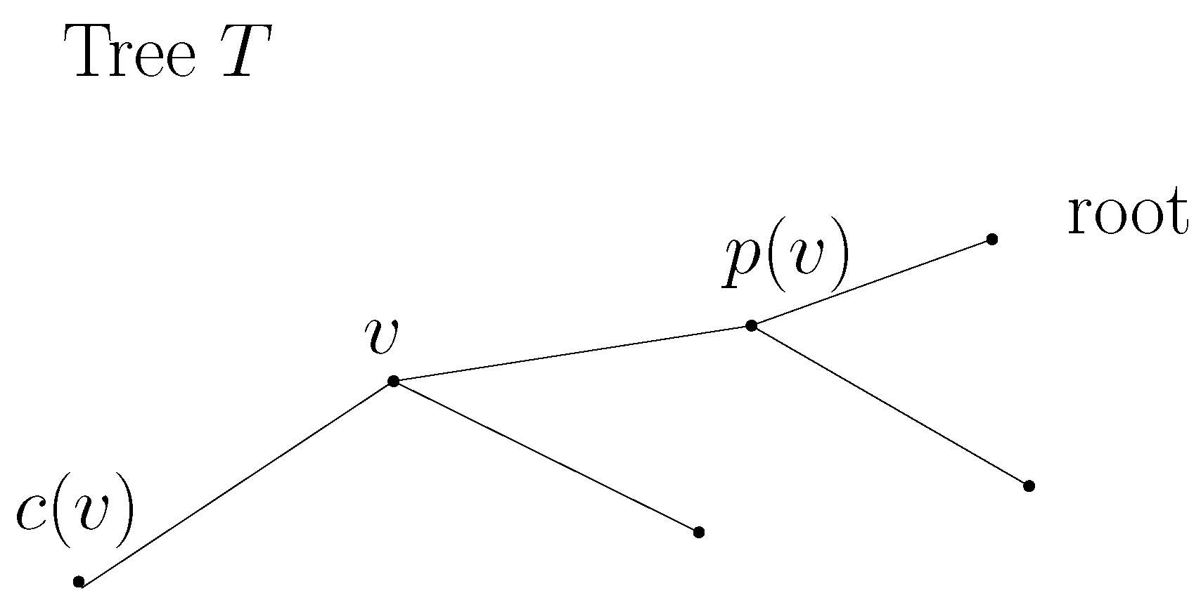
Proof. 

Suppose that u has been visiting UUVs along the path to $u_N$ in Algorithm 2. Let $PATH$ indicate the path for convenience. Suppose that $PATH$ consists of a set of UUVs $p_1\to p_2\to p_3\dots \to p_{end}$ in this order. Here, $p_{end}$ is the root $u_N$. As u moves along this path, it reaches the root in the end.

We first prove that $p_i$, where $i\in \{1,2,\dots ,end-1\}$, starts moving only after u encounters $p_i$. A UUV, other than a leaf starts moving only after all its descendants in T encounter it. Any UUV on $PATH$ is an ancestor of u. Hence, $p_i$ does not start moving before it encounters u.

In the case where u has just encountered $p_i$, u can sense $p_{i+1}$ utilizing its local sensors. Since u moves based on local sensing measurements, Algorithm 2 is distributed.

As u moves along $PATH$, it reaches the root in the end. We next prove that u remains connected to the root, during its maneuver along $PATH$ to the root. Consider the case where u has just encountered $p_i$ and starts moving towards $p_{i+1}$. In this case, u is connected to $p_{i+1}$. All UUVs in $p_{i+1}\to p_{i+2}\to p_{i+3}\dots \to p_{end}=u_N$ stand still. Hence, $p_{i+1}$ is connected to $u_N$. Since u is connected to $p_{i+1}$, u is also connected to $u_N$. It is proved that any UUV u remains connected to the root during its maneuver along $PATH$ to the root. □

4.3. Handling of Dynamic Scenarios, including Faulty UUVs

One may have a situation where a UUV is broken or the interaction link between two neighboring UUVs in T is broken by moving obstacles. Moreover, we may have a situation where an invisible UUV blocked by unknown obstacles appears suddenly. In these cases, every UUV stops moving, and we re-build a tree T utilizing Algorithm 1 in Section 4.1, so that network connectivity among UUVs can be re-established. Then, Algorithm 2 re-runs to achieve rendezvous at $u_N$. In this way, we can handle dynamic scenarios which may happen due to unknown obstacles.

As we re-build a tree T utilizing Algorithm 1 in Section 4.1, we may have a case where a tree T cannot be generated. This implies that a UUV may not be connected to the root, even after running Algorithm 1 in Section 4.1. For handling this case, we need to increase the number of neighbors for each UUV.

For handling the case where a UUV may not be connected to the root, we increase $P_0$ in Equation (5) for each UUV. As $P_0$ increases, the number of neighbors can increase, since a UUV $u_i$ is a neighbor to $u_j$ if $P\left(u_i\right)>P_{thres}$ and $P\left(u_j\right)>P_{thres}$. By increasing the signal emission strength, $u_i$ can detect a UUV that is located far from $u_i$. This emission power increase was also used in [41], for improving the network connectivity in multi-agent systems. We acknowledge that by increasing the signal emission strength, $u_i$ consumes more power.

4.3.1. Discard Faulty UUVs

Note that a UUV can become faulty owing to various reasons, such as hardware malfunction. We next address how to handle faulty UUVs. Let a healthy UUV denote a UUV having no faults.

Every UUV is encountered by its child under Algorithm 2. Thus, every faulty UUV, including a faulty root, can be detected by its child. Once a healthy UUV meets with a faulty UUV, the healthy UUV sends signal to the faulty UUV. A healthy UUV responds with an acknowledge signal whenever it receives a signal. If a UUV does not respond to the received signal, then the healthy UUV can find that a fault has occurred in the responding UUV.

Algorithm 2 is further designed to cope with a faulty UUV (including a faulty root). We discuss how to handle faulty UUVs from now on.

We first introduce a method of discarding (dropping) faulty UUVs once they are sensed. Once a broken UUV, e.g., $u_B$, is sensed, then a tree T is updated by applying Algorithm 1 in Section 4.1 without $u_B$. Thereafter, Algorithm 2 runs utilizing the updated T. The updated T does not contain $u_B$. This implies that we discarded (dropped) $u_B$.

If there are too many faulty UUVs, then it may be impossible to build a tree T without them. If we cannot build a tree without faulty UUVs, then we cannot make every healthy UUV encounter at the root UUV.

4.3.2. Using Static Faulty UUVs as Waypoints

There may be a case where a static faulty UUV has a communication ability, and thus, can emit a signal from it. We discuss a method which does not discard a static faulty UUV with communication ability. In this method, every UUV utilizes static faulty UUVs as “waypoints” along the path to the root UUV. Note that we do not discard faulty UUVs under this method.

Note that a healthy UUV, which does not have faults, can still measure the signal from a static faulty UUV. Assume that a healthy UUV, e.g., u, has a static faulty UUV, e.g., f, as its ancestor. In this case, the healthy UUV can still visit UUVs along the path, which contains f, to the root. This implies that u utilizes f as “waypoints” along the path to the root UUV.

Note that if f is healthy, then f waits until it encounters all its descendants. However, since f is faulty and static, f cannot move even after all its descendants encounter f. In this case, $p\left(f\right)$, the parent of f, cannot begin moving, since f is faulty and cannot move towards $p\left(f\right)$.

In order to resolve this problem, $p\left(f\right)$ removes f from its descendants list. In this way, $p\left(f\right)$ starts moving after all its descendants, other than f, encounter $p\left(f\right)$.

4.4. Visiting UUVs along the Path to the Root, Based on Signal Strength Measurements

At the beginning of Algorithm 2, Algorithm 1 in Section 4.1 runs to build a spanning tree T in a distributed manner. Algorithm 1 has the computational complexity $O\left(1\right)$ [61,62]. Once T is generated, the only control applied to each UUV is visiting UUVs along the path, e.g., $PATH$, to the root in T. This control is a high-level control of every UUV.

We introduce a local control to make one UUV visit UUVs along $PATH$ utilizing signal strength measurements. Consider the case where $PATH$ consists of a set of UUVs $p_1\to p_2\to p_3\dots \to p_{end}$ in this order. Here, $p_{end}$ is the root. In the inertial reference frame, let ${\mathbf{p}}_j\in {\mathbb{R}}^3$ indicate the 3D position of $p_j$ for convenience.

Suppose that $u_i$ encountered ${\mathbf{p}}_{j-1}\in {\mathbb{R}}^3$ and that the next UUV to encounter is ${\mathbf{p}}_j\in {\mathbb{R}}^3$. Since $u_i$ encountered ${\mathbf{p}}_{j-1}$, $u_i$ can detect the signal emitted from ${\mathbf{p}}_j$ utilizing its intensity sensors. Each intensity sensor on $u_i$ measures the strength of signals emitted from ${\mathbf{p}}_j$.

Signal field intensity is maximized at the signal source. See Equation (5) for RSSI. The gradient direction of a field defines the direction which maximizes the increase in the field. We let a UUV $u_i$ move in the gradient direction of the field. Since the gradient is the direction representing the maximum increase of the field, this maneuver makes the UUV move towards the signal source.

The gradient direction is measured in the body−fixed frame of $u_i$. In the body−fixed frame of $u_i$, let ${\mathbf{gr}}_i\left(P\right)\in {\mathbb{R}}^3$ present the gradient of P at the center of $u_i$. Moving in the direction of ${\mathbf{gr}}_i\left(P\right)$ makes $u_i$ move towards the signal source ${\mathbf{p}}_j$.

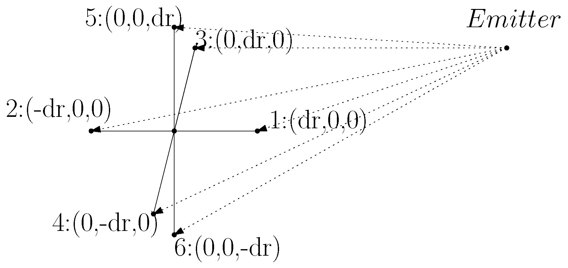
We next discuss how to derive ${\mathbf{gr}}_i\left(P\right)$ utilizing signal intensity measurements. The local coordinates of every intensity sensor are presented in Figure 3.

Assume that $\parallel {\mathbf{c}}_i^r\parallel$ is sufficiently small for all $r\in \{1,\dots ,6\}$. Through Taylor expansion up to the first-order derivative, one obtains the following:

$$\begin{array}{c}\hfill P\left({\mathbf{c}}_i^r\right)=P\left(u_i\right)+{\mathbf{c}}_i^r\ast {\mathbf{gr}}_i\left(P\right),\end{array}$$

(10)

which leads to:

$$\begin{array}{c}\hfill P\left({\mathbf{c}}_i^r\right)-P\left(u_i\right)={\mathbf{c}}_i^r\ast {\mathbf{gr}}_i\left(P\right).\end{array}$$

(11)

At each sampling step k, one obtains the following:

$$\begin{array}{c}\hfill {\mathbf{P}}_S=[P_c^1,P_c^2,\dots ,P_c^6].\end{array}$$

(12)

Here, $P_c^r=P\left({\mathbf{c}}_i^r\right)-P\left(u_i\right)$. Furthermore, we utilize the following:

$$\begin{array}{c}\hfill {\mathbf{C}}_S=[{\mathbf{c}}_i^1;{\mathbf{c}}_i^2;\dots {\mathbf{c}}_i^6].\end{array}$$

(13)

Utilizing (11)–(13), we derive the following:

$$\begin{array}{c}\hfill {\mathbf{P}}_S^T={\mathbf{C}}_S\ast {\mathbf{gr}}_i\left(P\right).\end{array}$$

(14)

Thereafter, ${\mathbf{gr}}_i\left(P\right)\in {\mathbb{R}}^3$ is derived using the pseudo-inverse as follows:

$$\begin{array}{c}\hfill {\mathbf{gr}}_i\left(P\right)={({\mathbf{C}}_S^T\ast {\mathbf{C}}_S)}^{-1}\ast {\mathbf{C}}_S\ast {\mathbf{P}}_S^T.\end{array}$$

(15)

where ${\mathbf{gr}}_i\left(P\right)\in {\mathbb{R}}^3$ defines the gradient of P, measured in the the body−fixed frame of $u_i$. In order to make $u_i$ head towards the signal source, the heading of $u_i$ is set as the gradient direction. Since the gradient is the direction representing the maximum increase of the field, this maneuver makes the UUV move towards the source.

In Equation (8), the UUV’s heading vector ${\mathbf{h}}_i\left(k\right)\in {\mathbb{R}}^3$ is defined in the inertial reference frame. Since ${\mathbf{gr}}_i\left(P\right)$ is defined in the body−fixed frame of $u_i$, one changes ${\mathbf{gr}}_i\left(P\right)$ into a gradient vector in the inertial reference frame.

Notice that $\mathbf{R}(\psi \left(k\right),\theta \left(k\right),\varphi \left(k\right))\ast \frac{{\mathbf{gr}}_i\left(P\right)}{\parallel {\mathbf{gr}}_i\left(P\right)\parallel }$ is a gradient vector in the inertial reference frame. In order to set the heading of $u_i$ as the gradient direction, $u_i$ sets its new heading using the following equation:

$$\begin{array}{c}\hfill {\mathbf{h}}_i(k+1)=\mathbf{R}(\psi \left(k\right),\theta \left(k\right),\varphi \left(k\right))\ast \frac{{\mathbf{gr}}_i\left(P\right)}{\parallel {\mathbf{gr}}_i\left(P\right)\parallel }.\end{array}$$

(16)

Note that a UUV does not have to measure its attitude $\varphi ,\theta ,\psi$ for moving towards the signal source. The UUV can move in the gradient direction ${\mathbf{gr}}_i\left(P\right)$ in its body−fixed frame. For instance, suppose that the gradient field ${\mathbf{gr}}_i\left(P\right)$ is estimated as [1,0,0] in the UUV’s body−fixed frame. Using (16), the UUV’s control command is generated for moving in the direction of [1,0,0] in its body−fixed frame.

We next discuss how $u_i$ can detect the moment when it encounters ${\mathbf{p}}_j$. If $P\left(u_i\right)$ in Equation (6) exceeds $P^e$ in Equation (7), then we assume that $u_i$ encountered ${\mathbf{p}}_j$. Thus, $u_i$ begins moving towards ${\mathbf{p}}_{j+1}$ if it exists.

For collision avoidance, we make $u_i$ slow down as it gets closer to $p_j$. The UUV’s linear speed $s_i\left(k\right)$ is set as follows. If $P\left(u_i\right)$ in Equation (6) is larger than $P^e$, then $u_i$ begins moving towards ${\mathbf{p}}_{j+1}$. Otherwise, we set the following:

$$\begin{array}{c}\hfill s_i\left(k\right)=min(s^{max},\beta \ast (P^e-P\left(u_i\right))).\end{array}$$

(17)

where $\beta >0$ is a tuning parameter. In MATLAB simulations, we use $\beta =10$. In Equation (17), $min(a,b)$ returns a smaller value between a and b.

When a UUV $u_i$ is sufficiently close to ${\mathbf{p}}_j\in {\mathbb{R}}^3$, it begins moving towards the next UUV ${\mathbf{p}}_{j+1}$. In this way, $u_i$ avoids collision with UUVs on its path to the root. In the case where $u_i$ encounters the root, $u_i$ stops moving.

This study considers a spherical UUV. The authors of [16,19,20,21] showed that by adopting vectored water jets, a spherical UUV can maneuver freely in any direction. The control of a spherical UUV appeared in [22], which used fuzzy PID controllers to independently control the robot’s movement in all directions.

While $u_i$ maneuvers, a moving obstacle may abruptly appear in practice. In this case, the UUV $u_i$ can avoid collision using reactive collision avoidance controls. We acknowledge that any reactive control method can be applied for this evasion [63,64,65].

5. Simulations

The MATLAB R2014a simulator is utilized to demonstrate the effectiveness of the proposed rendezvous controllers. The system environment includes Window 10, Intel Core ${}^{\mathrm{TM}}$ i5-7600K CPU@3.80 GHz. The controllers are implemented in a discrete-time system, and the sampling time interval to discretize the UUV’s velocity control (8) is 0.3 s.

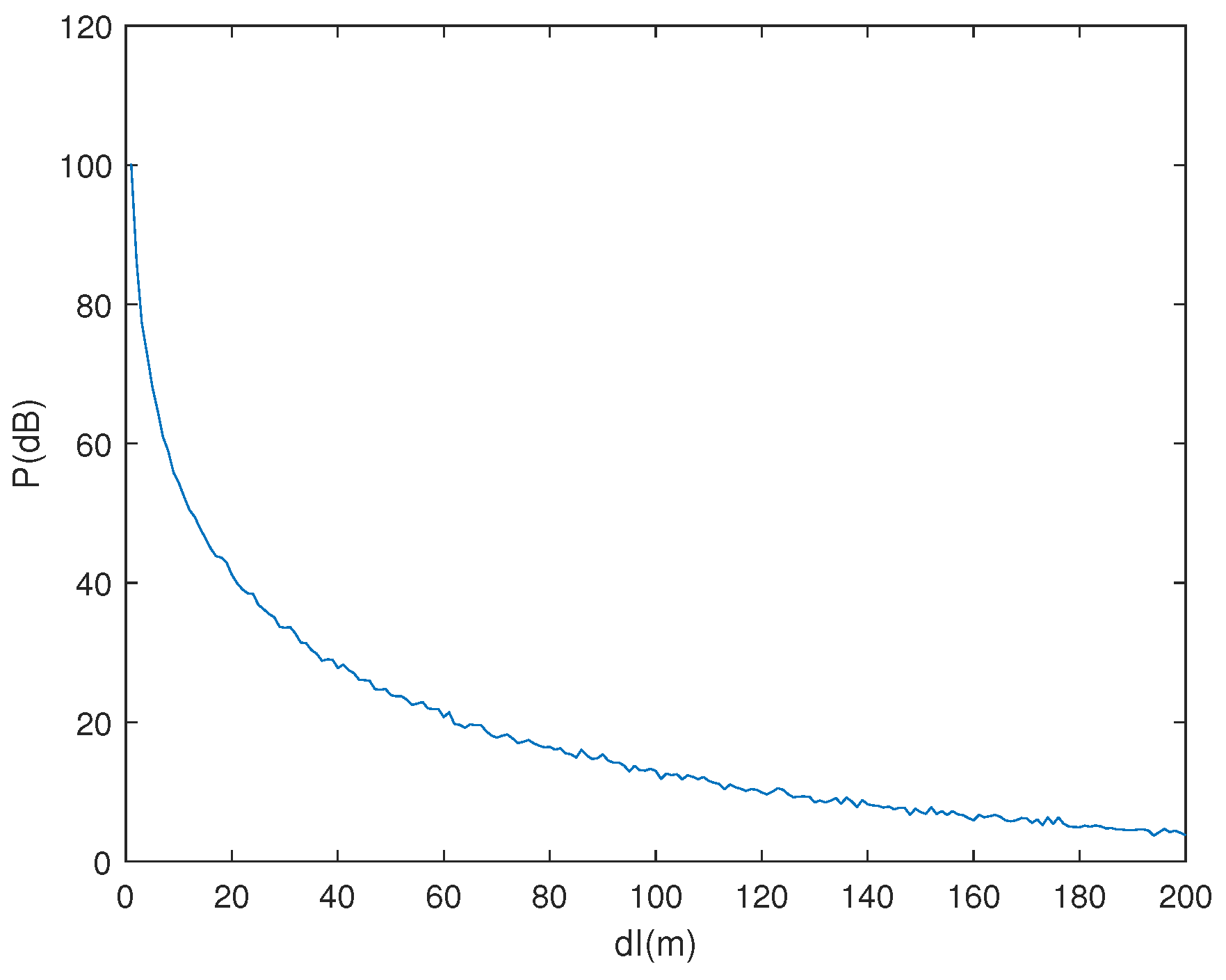
We simulate a 3D underwater environment (200 × 200 × 200) with many obstacles. For realistic simulations of the RSSI for an underwater emitter, we use the model parameters used in [28]. In Equation (5), $P_0$ = 100 dB, $E_p=2$, $\gamma =0.05$, and ${\sigma }^P=1$ are used, according to [28].

Recall that we said that a UUV $u_i$ is a neighbor to UUV $u_j$ if $P\left(u_i\right)>P_{thres}$ and $P\left(u_j\right)>P_{thres}$. We set $P_{thres}=52$ dB. Using Figure 4, the associated maximum sensing range $r_s$ is 10 m. In this way, the relative distance between two neighbor UUVs is less than 10 m.

The maximum speed of every UUV is set as $s^{max}=2$ (m/s). Recall that if $P(u_i,p_j)$ and $P(u_j,p_i)$ exceeds $P^e$, then we assume that $u_i$ encountered $p_j$. We set $P^e=100$ (in dB), which is identical to $P_0$. Using (7), $P^e=100$ (in dB) is associated with $ϵ=1$ m.

In this study, a UUV uses six intensity sensors. Figure 3 plots the local coordinates of every intensity sensors positioned on a UUV. $dr$ is the relative distance between the first sensor and any other sensor. $dr$ is a tuning parameter in our control.

If $dr$ is too small, then intensity measurements of six sensors on a UUV are not distinct from each other. In this case, the gradient direction at the UUV position cannot be estimated accurately. If $dr$ is too large, then we cannot apply the Taylor expansion in Equation (10). In the simulations, six intensity sensors are installed such that $dr=1$ m.

To prove the robustness of the proposed methods, we run 100 Monte Carlo (MC) simulations, such that the initial network satisfies this initial connectivity assumption. As far as we know, this initial connectivity assumption is required for any distributed rendezvous controls in the literature [34,41,51,52].

At the beginning of each MC simulation, 50 UUVs are randomly deployed until the following two conditions are met:

• No UUV is deployed inside an obstacle boundary.
• The deployed UUVs satisfy the initial connectivity assumption.

Once these two conditions are satisfied, then 50 UUVs begin to move under Algorithm 2. Otherwise, we keep deploying 50 UUVs until the above two conditions are met.

Once these two conditions are satisfied, then 50 UUVs begin to maneuver under Algorithm 2. This maneuver indicates the beginning of a single MC simulation. In all MC simulations, rendezvous is achieved for every UUV.

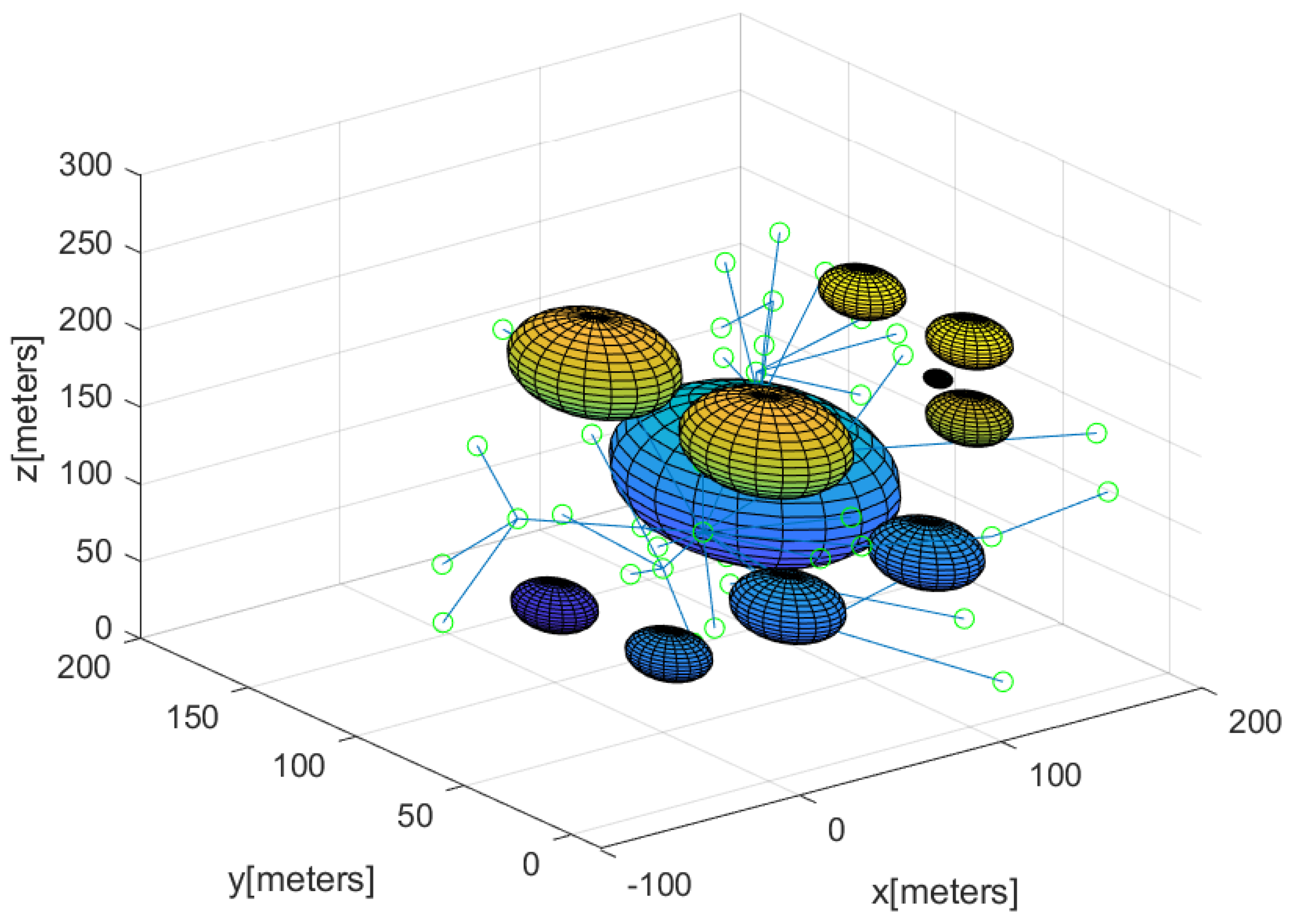
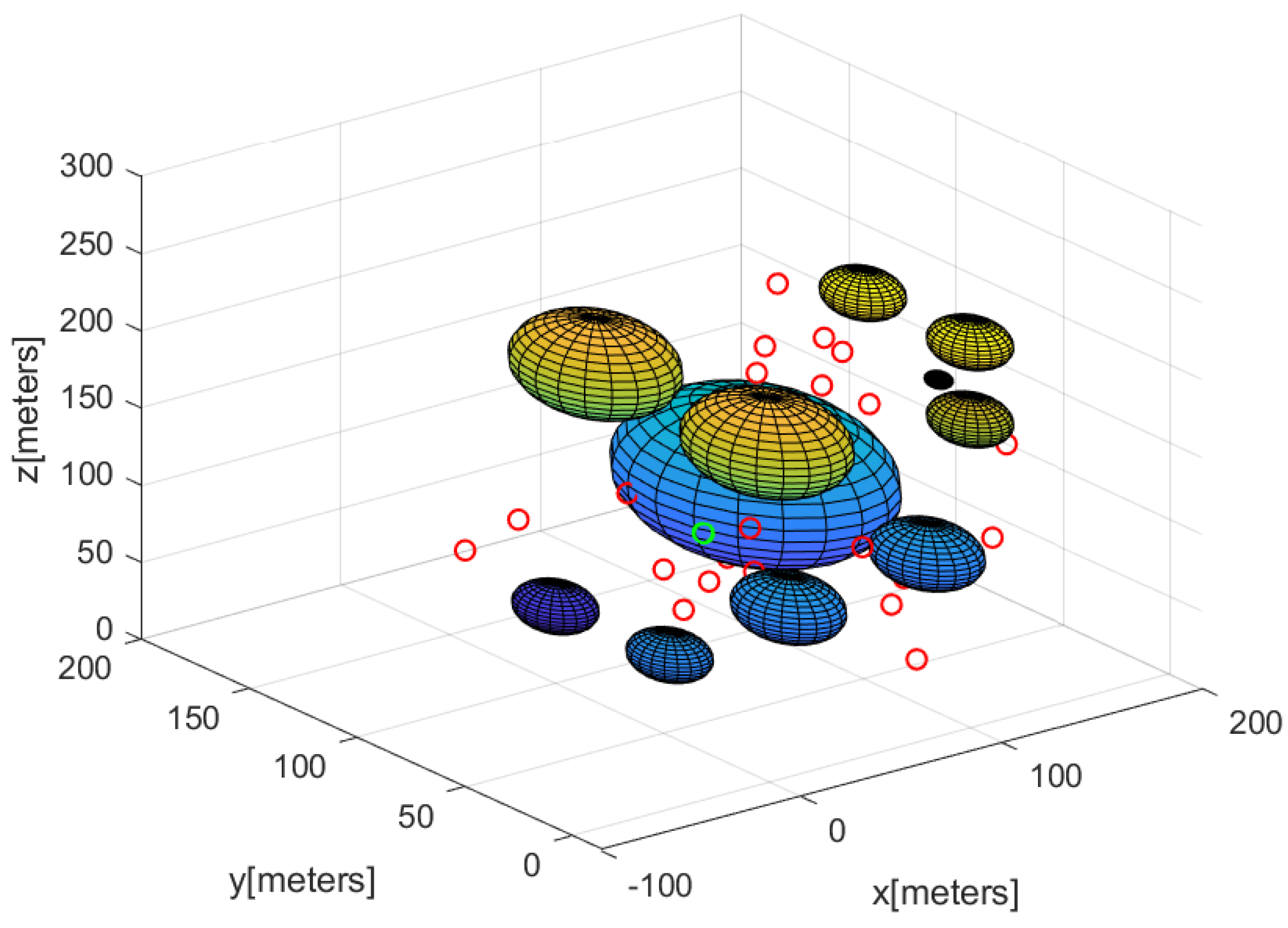
Considering one MC simulation, Figure 5 shows the initial position of every UUV. The initial position of every UUV is plotted with a green circle. This figure shows the obstacle boundaries with spheres. We also plot the tree graph T (blue line segments) generated initially.

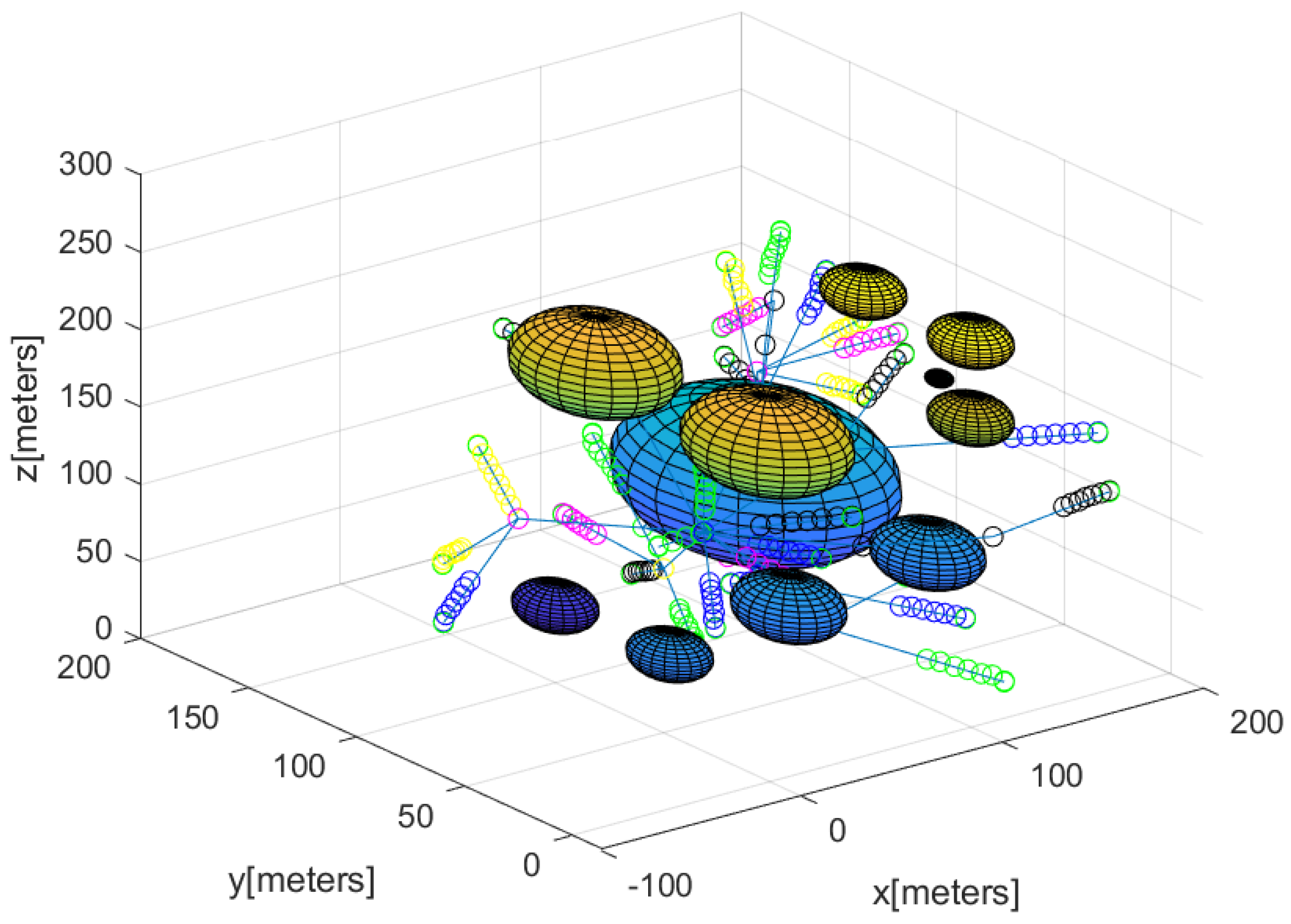
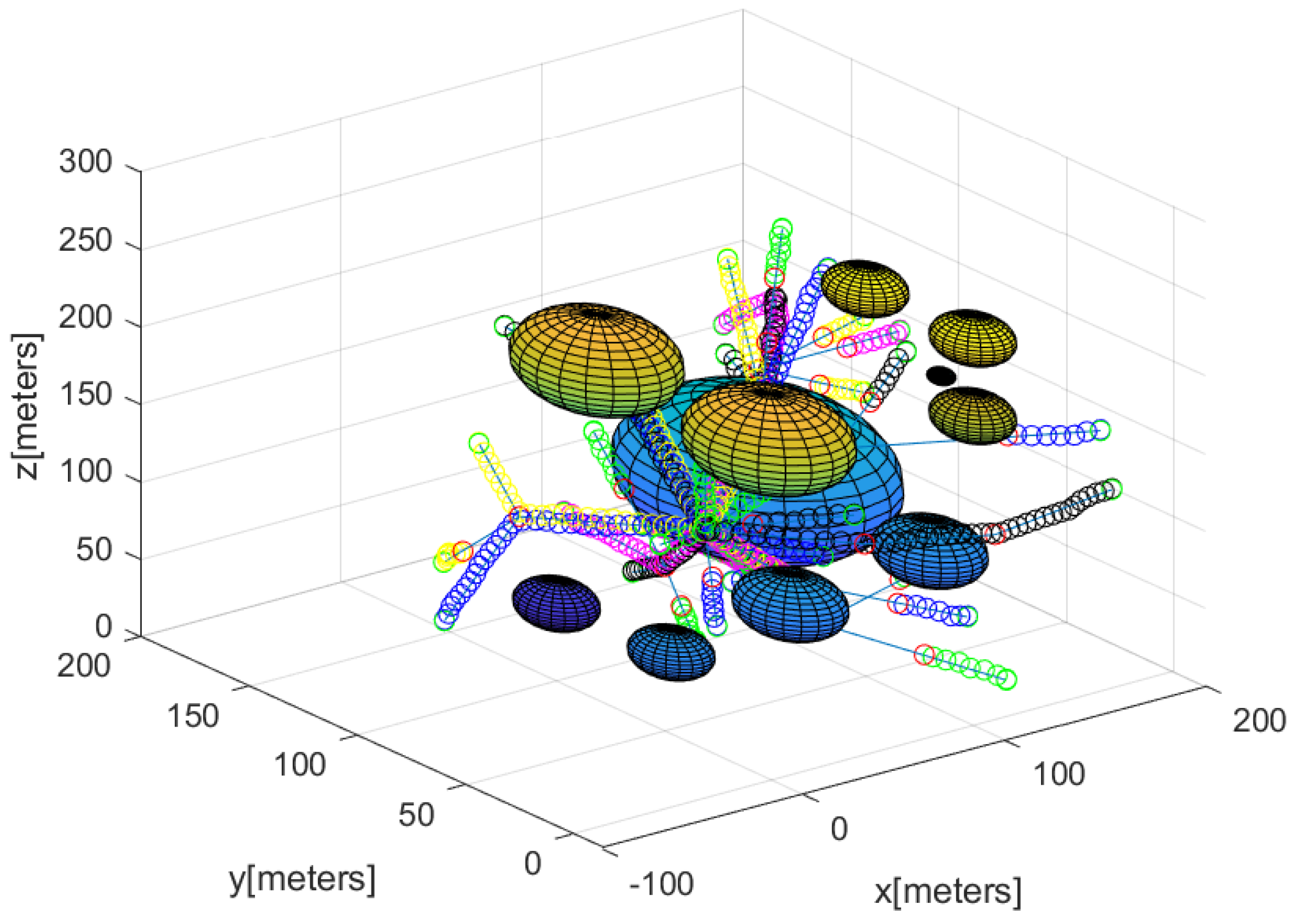
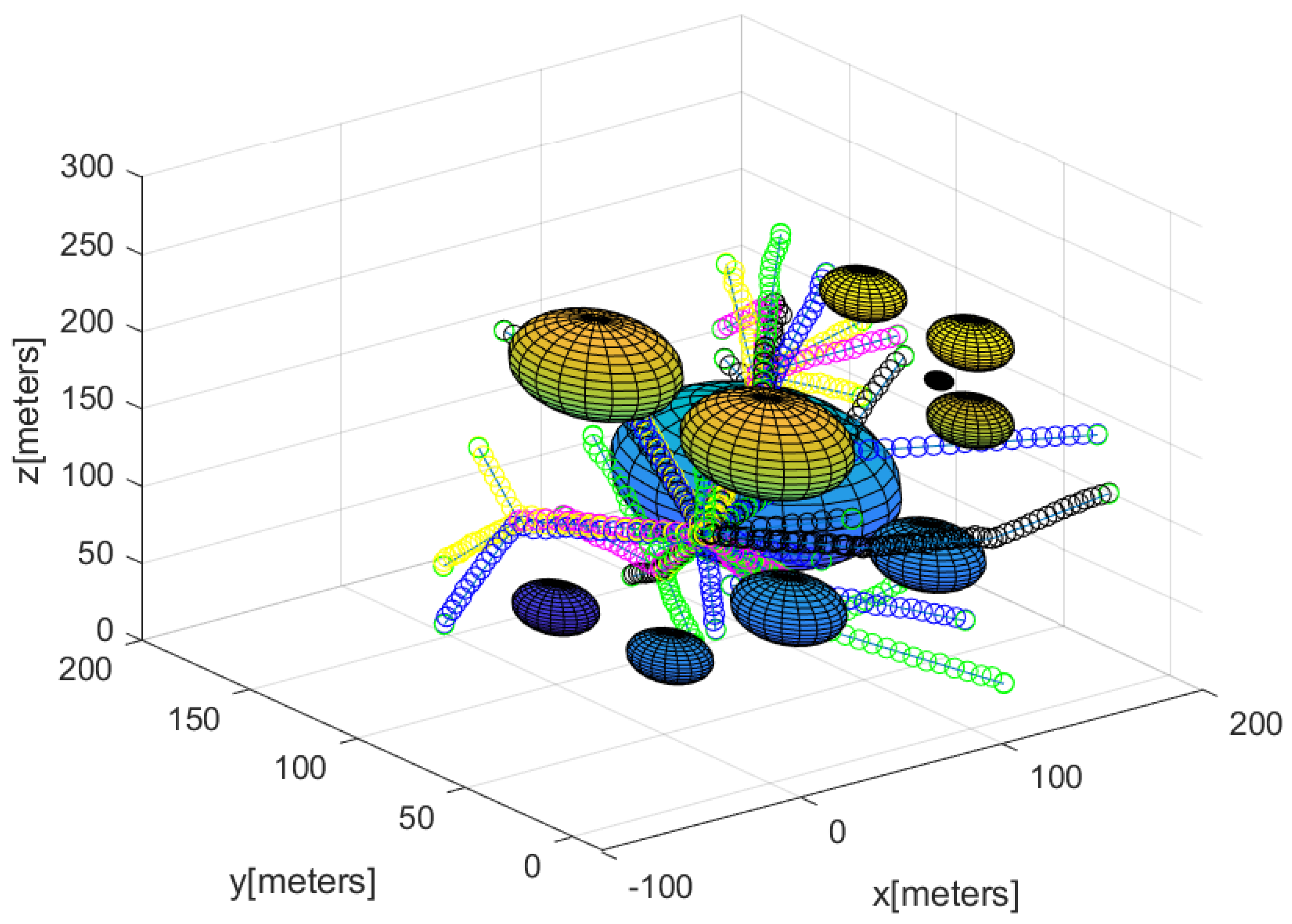
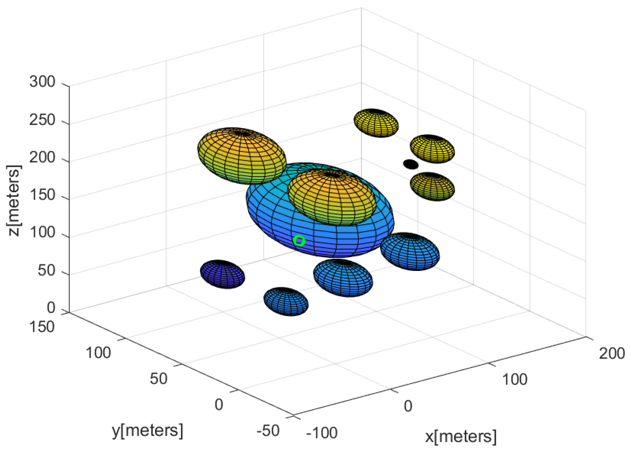
Figure 6 shows each UUV’s maneuver until $t=20$ s have passed. We also plot the tree graph T (blue line segments) generated at time 0. Every UUV’s maneuver is illustrated as circles with a distinct color. After 148 s have passed, all UUVs encounter at the root UUV while avoiding collision with obstacles. Figure 7 shows each UUV’s maneuver once the rendezvous is completed. Figure 8 shows the final position (green circle) of every UUV.

5.1. Using the Discard Approach in Section 4.3.1

We utilize the initial position of every UUV as in Figure 5. In this scenario, 25 UUVs among 50 UUVs are broken after 20 s have elapsed. Recall that Figure 6 shows each UUV’s maneuver until $t=20$ s pass.

To handle broken UUVs, we utilize the discard approach in Section 4.3.1. Considering one MC simulation, Figure 9 plots every UUV’s maneuver until $t=20$ s have passed. In this figure, every UUV’s maneuver is illustrated as circles with a distinct color. At $t=0$ s, we build a tree T (blue line segments in Figure 9) containing all UUVs. At $t=20$ s, 25 broken UUVs are illustrated with red circles in Figure 9. At $t=20$ s, we re-build a connected tree T without broken UUVs. The re-built tree T is marked with red line segments in Figure 9.

Considering UUVs’ faults, Figure 10 and Figure 11 show the movement of every UUV under our 3D distributed rendezvous controllers. In the figures, every UUV’s maneuver is illustrated as circles with a distinct color. In total, 25 broken UUVs are illustrated with red circles. To handle broken UUVs, one utilizes the discard approach in Section 4.3.1. In total, 25 healthy UUVs spend 180 s to encounter at the root, while avoiding collision with obstacles. Figure 11 shows every UUV’s final position (green circles) after the rendezvous is completed (discard approach is utilized). A total of 25 broken UUVs are illustrated with red circles.

5.2. Using the Waypoint Approach in Section 4.3.2

We utilize the initial position of every UUV as in Figure 5. In this scenario, 25 UUVs among 50 UUVs are broken after 20 s have elapsed. Recall that Figure 6 shows each UUV’s maneuver until $t=20$ s pass.

Considering UUVs’ faults, Figure 12 and Figure 13 show the movement of every UUV under our 3D distributed rendezvous controllers. In the figures, every UUV’s maneuver is illustrated as circles with a distinct color. To handle broken UUVs, we utilize the waypoint approach in Section 4.3.2. At $t=0$ s, we build a tree T (blue line segments in Figure 12) containing all UUVs. A total of 25 broken UUVs are illustrated with red circles. In Figure 13, all healthy UUVs (green circles) rendezvous at the root. We can see that healthy UUVs use broken UUVs as waypoints for reaching the root. A total of 25 healthy UUVs spend 148 s to encounter at the root UUV, while avoiding collision with obstacles.

6. Conclusions

This article proposed distributed rendezvous controllers to solve the multi-robot rendezvous problem in cluttered 3D environments without GPS. The proposed 3D rendezvous controls assure the convergence to the root, while maintaining the connectivity of the time-varying and position-dependent communication network.

This study considers multiple UUVs such that each UUV has multiple signal intensity sensors surrounding it. Multiple intensity sensors on a UUV can measure the strength of signals, and the UUV moves based on the signal strength measurements. Our rendezvous algorithms are robust to faults in the system. This study proves the convergence of the proposed rendezvous algorithms and demonstrates the effectiveness of the proposed algorithms utilizing MATLAB simulations.

Note that the proposed rendezvous algorithms do not rely on the dimension (2D or 3D) of the environment. This implies that our algorithms can be applied for the rendezvous problem of autonomous aerial vehicles, autonomous underwater vehicles, or autonomous ground vehicles. In future studies, we will perform experiments utilizing real UUVs to verify the effectiveness of the proposed rendezvous algorithms.