
Segmentation and Classification of Zn-Al-Mg-Sn SEM BSE Microstructure

Abstract
:1. Introduction
- topographic contrast—dominantly the SE signal, which is more sensitive to the 3D topography of the surface of the scanned sample;
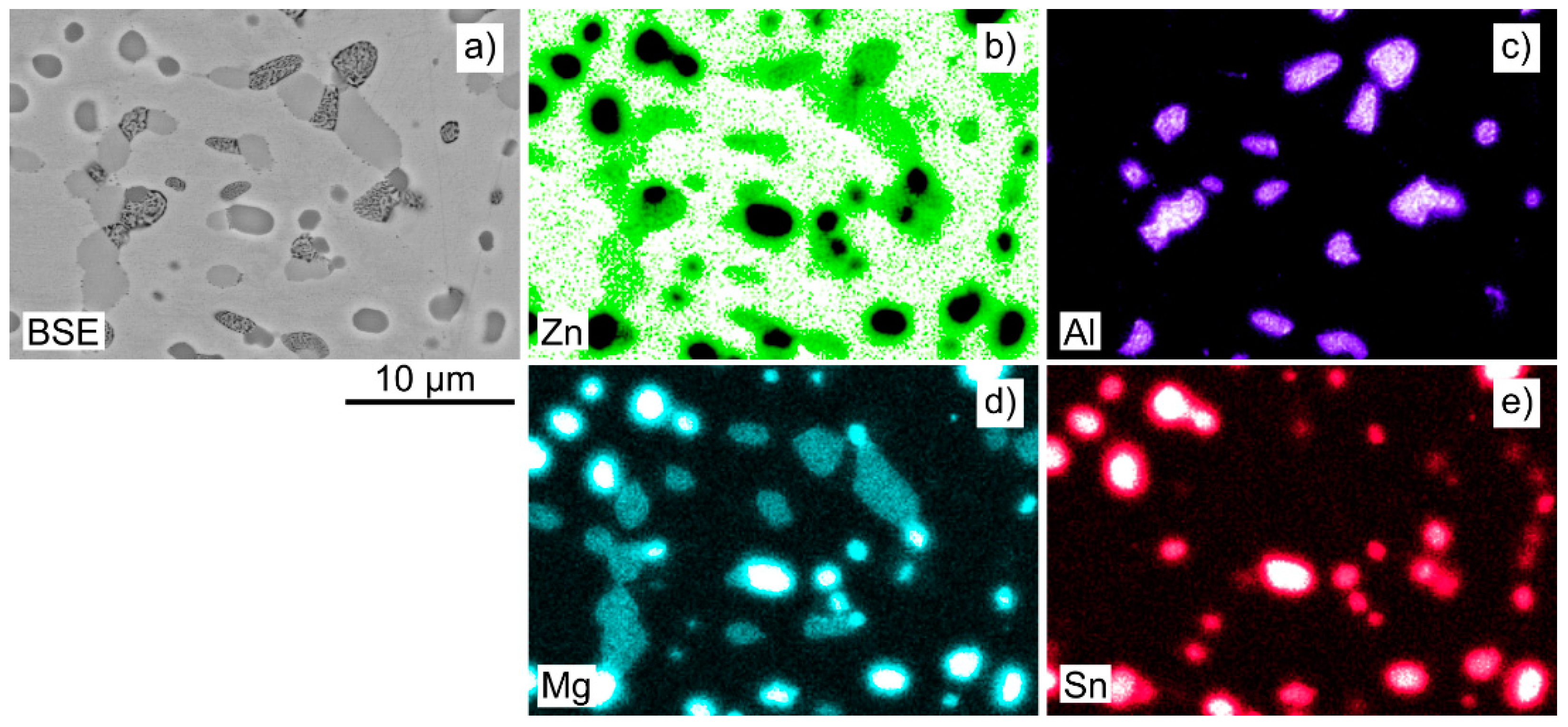
- composition contrast—dominantly the BSE signal, which is more dependent on the atomic number of the individual atoms in the sample;
- channelling contrast—electrons from the beam penetrate more easily along the crystal lattice than in a random orientation.
- time and effort requirements;
- subjective errors (bias) and related repeatability;
- need for domain knowledge in the form of technological expertise.
- 1st trend—signal processing: noise removal and texture analysis;
- 5th trend—collaborative microscopy: complementary imaging modalities;
- 8th trend—semi-automation: creating training data for DL;
- 9th trend—interdisciplinary cooperation: assessing the properties of image material.
- Understand the characteristics of the visual data from the modality SEM BSE (rich visual content). The chosen alloy has not been so far investigated through this approach (Sn content, zoom);
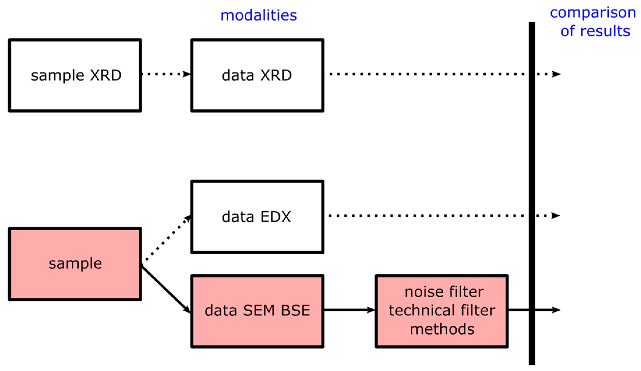
- Remove the bottleneck in the technological workplace—see Figure 1. The resolution, noise level and data acquisition time (compared to EDX) clearly speak in favour of the presented approach. The modality XRD is relatively fast, but it does not provide any visual data, just the numerical values of the phase quantification (PQ);
- Quickly process the sample and acquire a lot of information from a large surface. From these visual data, it is possible to find out more details regarding manifestation of the metallurgical process, chemical composition, semantics of the scene, class imbalance, etc.;
- Save time and energy for the preparation of training data for deep learning compared to the manual editing from scratch;
- Process the previously taken image documentation even if the sample does not exist anymore.
2. Materials and Methods
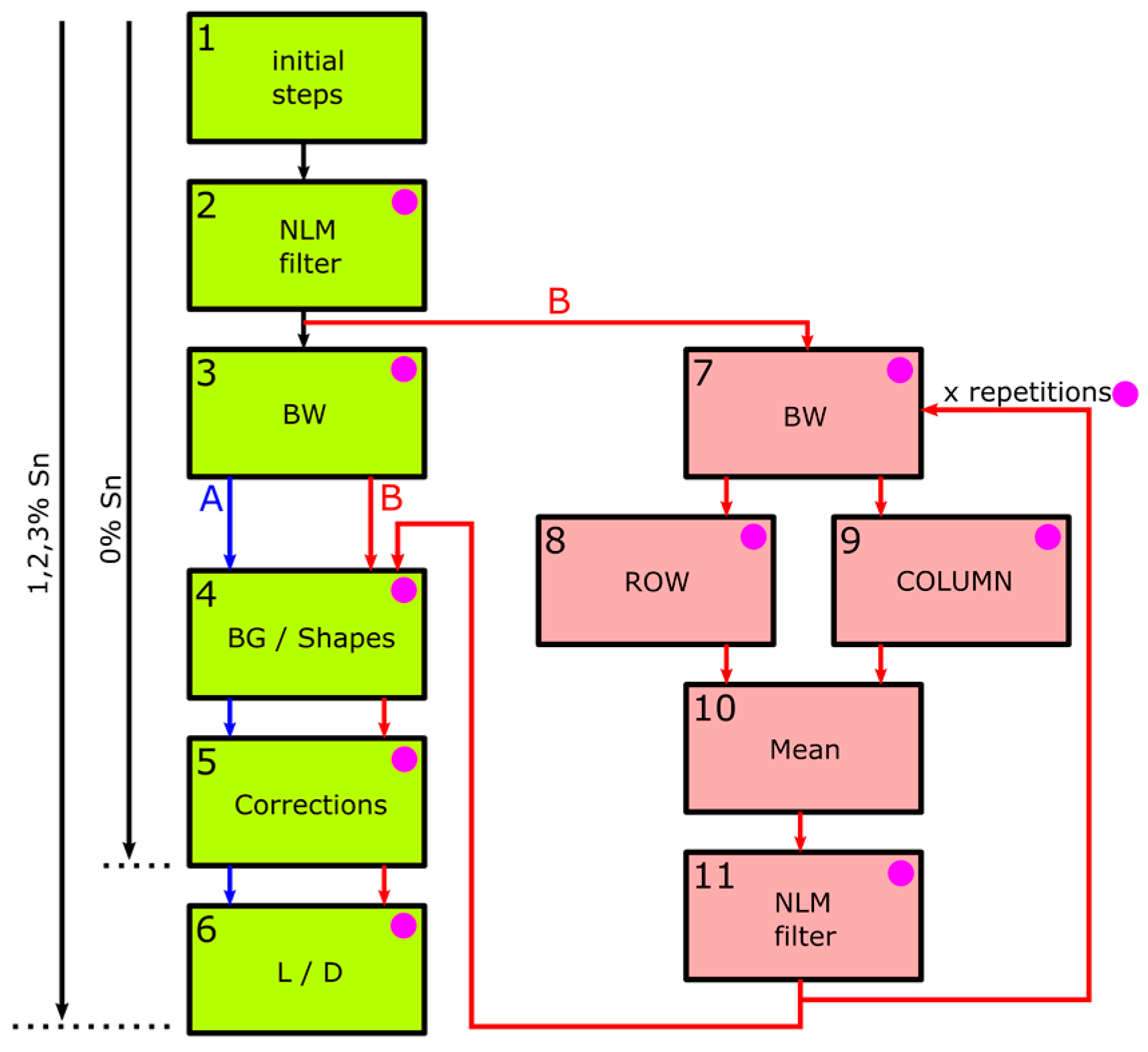
- Initial steps—the selection of the pure image information, its conversion to the single-precision floating point type and extraction of the zoom and %Sn information;
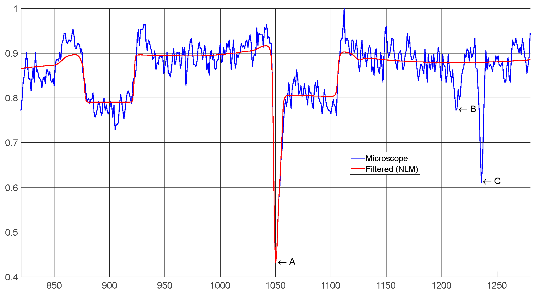
- NLM filter—the applying of several consecutive NLM filters to remove noise. Function: imnlmfilt. The incorrectly selected configuration values result in poor noise removal or, on the contrary, loss of important edges of shapes. It is therefore necessary to pay sufficient attention to this step. Configuration values: DegreeOfSmoothing (DOS), SWS, ComparisonWindowSize (CWS);
- BW—the classification of the first BW segment. The classification of the BW shapes can be divided first into level thresholding, when according to a priori statistically obtained value, which is sufficiently low, the dark BW components are identified. These are subsequently expanded using the morphological operations imfill and imclose with a suitably chosen structuring element, completed and closed with the white BW components. Configuration values: intensity level threshold to black, type and size of the structuring element;
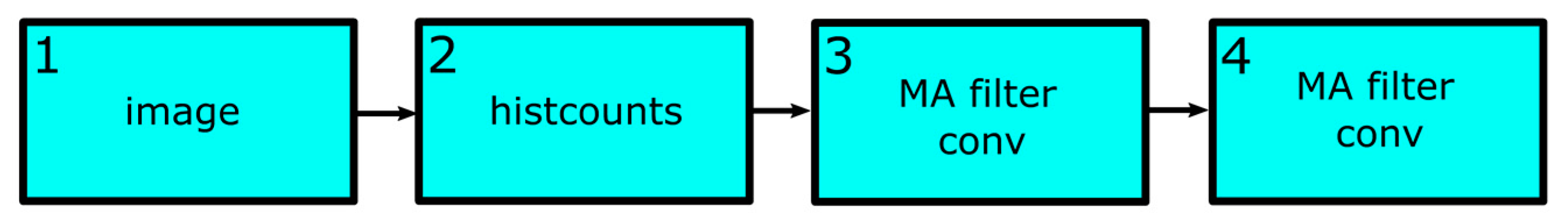
- BG/Shapes—the separation and classification of the BG background from L + D shapes. Method: histogram thresholding. Configuration values: intensity histogram threshold, moving average (MA) filter parameters and number of sequential filtering;
- Corrections—the optional step where some pixels can be swapped between the BG segments and L + D Shapes (such as precipitates). Functions: bwconncomp to obtain the connected components with the default connectivity 8, regionprops(‘Area’) for obtaining the number of pixels in connected shapes. Configuration values: number of pixels in connected shapes;
- L/D—this step occurs only in case of nonzero Sn content. Method: histogram thresholding. The data, left over from the previous segmentations, are divided into the L and D shapes. Configuration values: intensity histogram threshold, MA filter parameters and number of sequential filtering.
- 7.
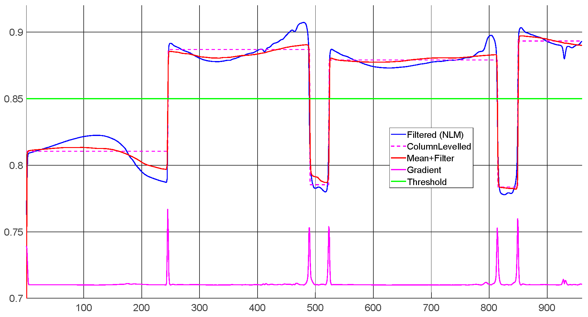
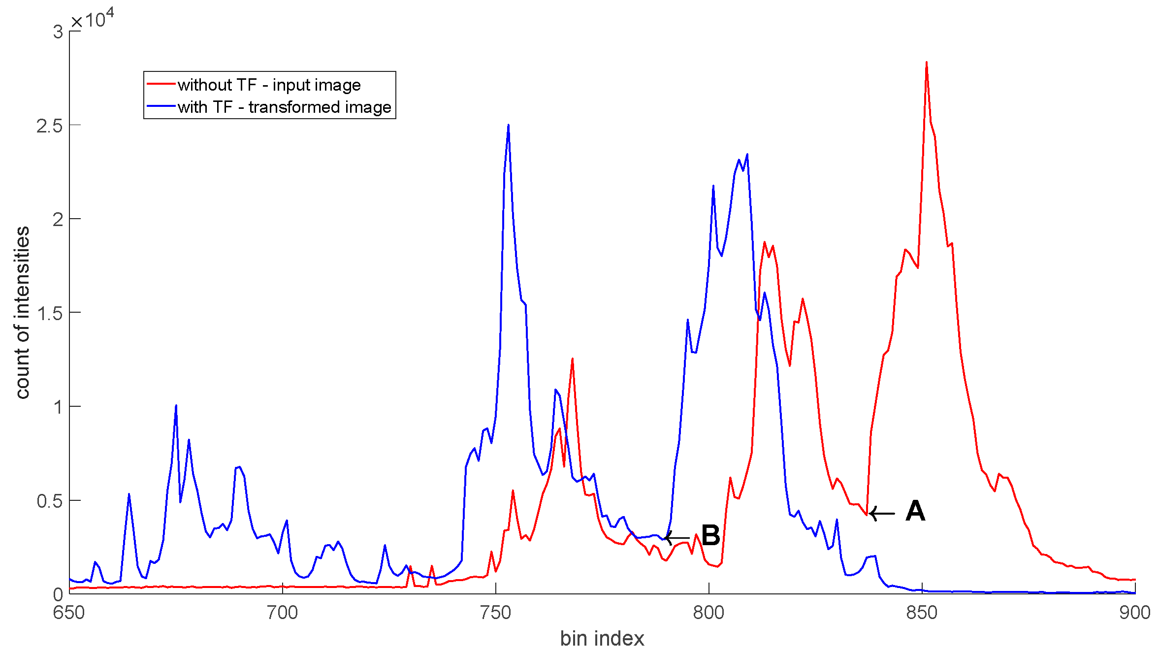
- BW—all values of the identified BW segment can be intensively adjusted to another level (e.g., 0). This will eliminate the problems with large and sudden intensity changes within the BW segment (see e.g., Figure 5 indices between 600 and 720). These would be difficult to process in the steps based on gradients—blocks 8 and 9. Configuration values: intensity level threshold to black, type and size of the structuring element, setting a constant intensity level;
- 8.
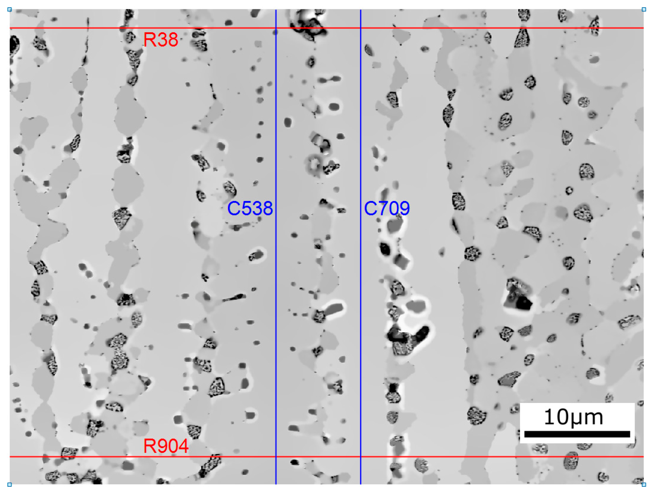
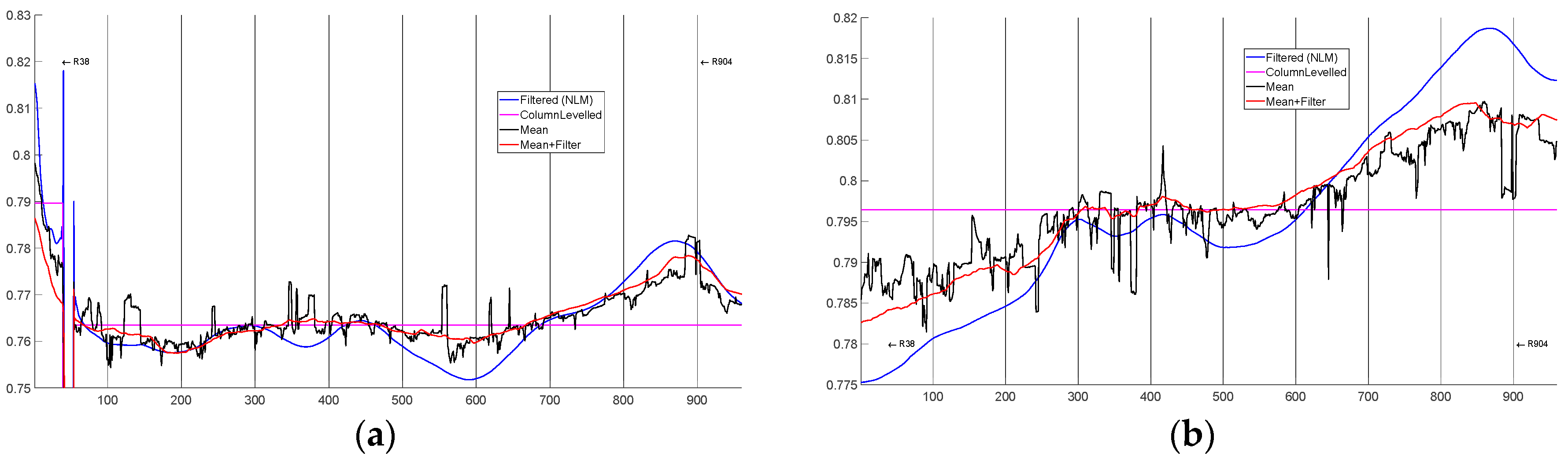
- ROW—the image is levelled row by row. With the preselected absolute value of the gradients, the local extremes of the gradients are identified (see Figure 6). Between two such extremes, the pixels’ intensities of the given section are levelled. Configuration values: selection level of the absolute local extremes of gradients;
- 9.
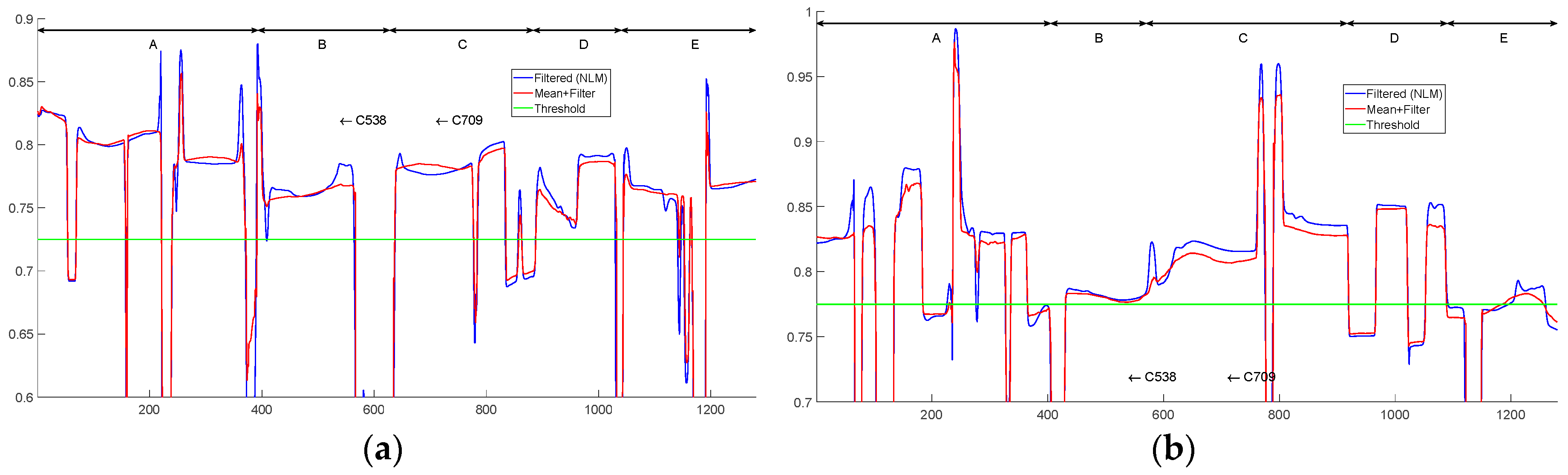
- COLUMN—analogous to block 8, only the columns are involved. With the preselected absolute value of the gradients, the local extremes of the gradients are identified (see Figure 6). Between two such extremes, the pixels’ intensities of the given section are levelled. Configuration values: selection level of the absolute local extremes of gradients;
- 10.
- Mean—the arithmetic mean of two images (levelled in the direction of rows and columns in blocks 8 and 9) is calculated. The nature of the data in both directions can sometimes differ significantly. An important role here is played by the sharpness of the edges and the intensity distance between the individual levels (contrast between the shapes). Overall, with sufficient sharpness and contrast, there is no damage to the contours of the shapes, and the gradual application of the technical filter results in the levelling of the inside of the shapes;
- 11.
- NLM filter—the result from the previous step is jagged and therefore needs to be smoothed. The filter parameters may or may not be the same as the parameters from block 2. Configuration values: DOS, SWS, CWS.
3. Results and Analysis
- 3.2: Procedure B from Figure 7—one particular image was chosen from Section 3.1 (the image of 1% Sn and Zoom4000). The simple application of the technical filter improved the accuracy from 92% to 94%. Again, there was no manual tuning of configuration values. The duration of the image analysis was longer than the time required by the application of the NLM filter (part of the technical filter: block 11, Figure 7);
- 3.3: Demanding image (tuning of the configuration values)—a demanding image of 1% Sn and Zoom2000, outside of the selection from Section 3.1, was chosen to demonstrate the complexity of the visual content. Multiple backgrounds were presented. Now, the configuration values (inclusive of the technical filter) were manually tuned. The accuracy had been improved from 79% to 92%.
- 3.4: Comparison of results with the XRD data—a set of 180 images were analysed. Most of them were processed with the preset configuration values. Minority of them had to be manually tuned. The value of the accuracy improvement could reach up to 20%. The XRD data were used just as a benchmark. They were not needed in actual analysis.
3.1. Procedure A from Figure 7
3.2. Procedure B from Figure 7 (the Technical Filter)
3.3. Demanding Image (Tuning of the Configuration Values)
3.4. Comparison of Results with the XRD Data
4. Discussion
- Flat and wide valleys;
- Two peaks characterised by significantly different heights (a problematically detectable valley);
- Noise in the histogram;
- Noisy spikes;
- Overlapping distributions of BG and the object;
- The object represented in a small percentage;
- BG consisting of several regions.
- All segmentation areas are classified at the same time;
- Everything on one side from the threshold level automatically falls into one segment/class, and thus the problem with oversegmentation is eliminated (see the white rim described in Figure 3);
- Adaptability to changes in brightness (horizontal shift of the histogram);
- The same sense of all intensity values in the image (global thresholding), which, however, can easily turn into a disadvantage if the histogram deployment conditions are not observed.
- Small erosion of less sharp shape edges (especially with multiple uses of the filter);
- Segmentation line artefacts occurring if the gradient level was incorrectly determined;
- Different effects at the different zoom levels and Sn content;
- No recommendation for the number of repetitions.
- High resolution;
- Extreme variability in texture and shapes;
- Significantly fragmented images with often unclear boundaries of displayed objects;
- Unbalanced classes (unequal percentage representation on the image);
- Absence of prior structural information.
5. Conclusions
Author Contributions
Funding
Institutional Review Board Statement
Informed Consent Statement
Data Availability Statement
Conflicts of Interest
References
- Ul-Hamid, A. A Beginners’ Guide to Scanning Electron Microscopy; Springer Nature: Cham, Switzerland, 2018; pp. 15–76, 83, 309–358. [Google Scholar]
- Goldstein, J.I.; Newbury, D.E. Scanning Electron Microscopy and X-ray Microanalysis, 4th ed.; Springer Science + Business Media LLC: New York, NY, USA, 2018; pp. 2, 15–37. [Google Scholar]
- Amelinckx, S.; van Dyck, D. Electron Microscopy Principles and Fundamentals; VCH Verlagsgesellschaft mbH: Weinheim, Germany, 1997; p. 315. [Google Scholar]
- Bowen, D.K.; Hall, C.R. Microscopy of Materials Modern Imaging Methods Using Electron, X-ray and Ion Beams; The MacMillan Press LTD: London, UK, 1975; p. 7. [Google Scholar]
- Dehm, G.; Howe, J.M. In-Situ Electron Microscopy Applications in Physics, Chemistry and Materials Science; Wiley-VCH Verlag & Co. KGaA: Weinheim, Germany, 2012; pp. 19–44. [Google Scholar]
- Geels, K.; Fowler, D.B. Metallographic and Materialographic Specimen Preparation, Light Microscopy, Image Analysis and Hardness Testing; ASTM International: West Conshohocken, PA, USA, 2007; pp. 1–521. [Google Scholar]
- Lyman, C.E.; Newbury, D.E. Scanning Electron Microscopy, X-Ray Microanalysis, and Analytical Electron Microscopy A Laboratory Workbook; Plenum Press: New York, NY, USA, 1990; pp. 159–171. [Google Scholar]
- Murr, L.E. Electron and Ion Microscopy and Microanalysis Principles and Applications, 2nd ed.; CRC Press: Boca Raton, FL, USA, 2018; pp. 711–752. [Google Scholar]
- Echlin, P. Handbook of Sample Preparation for Scanning Electron Microscopy and X-ray Microanalysis; Springer Science + Business Media, LLC: New York, NY, USA, 2009; pp. 235–299. [Google Scholar]
- Wojnar, L. image analysis Applications in Materials Engineering; CRC Press: Boca Raton, FL, USA, 1999; pp. 90, 130, 221. [Google Scholar]
- Abbaschian, R.; Abbaschian, L. Physical Metallurgy Principles, 4th ed.; Cengage Learning: Boston, MA, USA, 2009; p. 175. [Google Scholar]
- Laughlin, D.E.; Hono, K. Physical Metallurgy Volume 2, 5th ed.; Elsevier B.V.: Amsterdam, The Netherlands, 2014; p. 1073. [Google Scholar]
- Cahn, R.W.; Haasen, P. Physical Metallurgy Volume 1, 4th ed.; Elsevier Science B.V.: Amsterdam, The Netherlands, 1996; p. 921. [Google Scholar]
- Lakhtin, Y. Engineering Physical Metallurgy; S. K. Jain for CBS Publishers & Distributors: New Delhi, India, 1998; p. 49. [Google Scholar]
- Russ, J.C. Image Analysis of Food Microstructure; CRC Press: Boca Raton, FL, USA, 2005; pp. 74, 215. [Google Scholar]
- Ercetin, A.; Akkoyun, F. Image Processing of Mg-Al-Sn Alloy Microstructures for Determining Phase Ratios and Grain Size and Correction with Manual Measurement. Materials 2021, 14, 5095. [Google Scholar] [CrossRef] [PubMed]
- Chalusiak, M.; Nawrot, W. Swarm Intelligence-Based Methodology for Scanning Electron Microscope Image Segmentation of Solid Oxide Fuel Cell Anode. Energies 2021, 14, 3055. [Google Scholar] [CrossRef]
- Holm, E.A.; Cohn, R. Overview: Computer vision and machine learning for microstructure characterization and analysis. Met. Mater. Trans. A 2020, 51, 5985–5999. [Google Scholar] [CrossRef]
- Campbell, A.; Murray, P. New methods for automatic quantification of microstructural features using digital image processing. Mater. Des. 2018, 141, 395–396. [Google Scholar] [CrossRef] [Green Version]
- Luengo, J.; Moreno, R. A tutorial on the segmentation of metallographic images: Taxonomy, new MetalDAM dataset, deep learning-based ensemble model, experimental analysis and challenges. Inf. Fusion 2022, 78, 232–253. [Google Scholar] [CrossRef]
- Argyriou, V.; del Rincón, J.M. Image, Video & 3D Data Registration Medical, Satellite & Video Processing Applications with Quality Metrics; John Wiley & Sons Ltd: Chichester, UK, 2015; p. 5. [Google Scholar]
- Drouyer, S. 3D Topography by Image Segmentation Approach: Application to Scanning Electron Microscopy. Topographie 3D Par Approche Segmentation: Application Au Microscope électronique à Balayage. Ph.D. Thesis, Université Paris sciences et lettres, Paris, France, 2017; p. 22. [Google Scholar]
- Mavrogonatos, A.; Papia, E.-M. Measuring the randomness of micro- and nanostructure spatial distributions: Effects of Scanning Electron Microscope image processing and analysis. J. Microsc. 2022, 289, 48–57. [Google Scholar] [CrossRef]
- Burger, W.; Burge, M.J. Principles of Digital Image Processing Fundamental Techniques; Springer: London, UK, 2009; p. 119. [Google Scholar]
- Boyat, A.K.; Joshi, B.K. A Review Paper: Noise Models in Digital Image Processing. arXiv 2015, arXiv:1505.03489. [Google Scholar] [CrossRef]
- Marturi, N.; Dembélé, S. Scanning electron microscope image signal-to-noise ratio monitoring for micro-nanomanipulation. J. Scanning Microsc. 2014, 36, 419–429. [Google Scholar] [CrossRef] [Green Version]
- Prasad, M.S.; Joy, D.C. Is SEM Noise Gaussian? Microsc. Microanal. 2003, 9, 982–983. [Google Scholar] [CrossRef] [Green Version]
- Paris, S.; Hasinoff, S.W. Local Laplacian Filters: Edge-aware Image Processing with a Laplacian Pyramid. ACM Trans. Graph. 2015, 30, 68. [Google Scholar] [CrossRef]
- Buades, A.; Coll, B. A non-local algorithm for image denoising. In Proceedings of the 2005 IEEE Computer Society Conference on Computer Vision and Pattern Recognition (CVPR’05), San Diego, CA, USA, 20–25 June 2005; pp. 60–65. [Google Scholar] [CrossRef]
- Aubry, M.; Paris, S. Fast Local Laplacian Filters: Theory and Applications. ACM Trans. Graph. 2014, 33, 2. [Google Scholar] [CrossRef] [Green Version]
- Tomasi, C.; Manduchi, R. Bilateral Filtering for Gray and Color Images. In Proceedings of the 1998 IEEE International Conference on Computer Vision, Bombay, India, 4–7 January 1998; pp. 1–2. [Google Scholar] [CrossRef]
- Bonnet, N. Some trends in microscope image processing. Micron 2004, 35, 635–649. [Google Scholar] [CrossRef] [PubMed]
- Bhanu, B.; Lee, S. Genetic Learning for Adaptive Image Segmentation; Springer Science + Business Media: New York, NY, USA, 1994; pp. 1–14. [Google Scholar]
- Gong, S.; Liu, C. Advanced Image and Video Processing Using Matlab; Springer International Publishing AG: Cham, Switzerland, 2019; p. 65. [Google Scholar]
- Siddiqui, F.U.; Yahya, A. Clustering Techniques for Image Segmentation; Springer Nature: Cham, Switzerland, 2022; p. 3. [Google Scholar]
- Yoo, T.S. Insight into Images Principles and Practice for Segmentation, Registration, and Image Analysis; A K Peters, Ltd.: Natick, MA, USA, 2004; p. 362. [Google Scholar]
- Gogola, P.; Gabalcová, Z. The Effect of Sn Addition on Zn-Al-Mg Alloy; Part I: Microstructure and Phase Composition. Materials 2021, 14, 5404. [Google Scholar] [CrossRef] [PubMed]
- Gabalcová, Z.; Gogola, P. The Effect of Sn Addition on Zn-Al-Mg Alloy; Part II: Corrosion Behaviour. Materials 2021, 14, 5290. [Google Scholar] [CrossRef] [PubMed]
- Truglas, T.; Duchoslav, J. Correlative characterization of Zn-Al-Mg coatings by electron microscopy and FIB tomography. Mater. Charact. 2020, 166, 1–8. [Google Scholar] [CrossRef]
- Li, C.; Wang, D. Application of Machine Learning Techniques in Mineral Classification for Scanning Electron Microscope—Energy Dispersive X-Ray Spectroscopy (SEM-EDS) Images. J. Pet. Sci. Eng. 2021, 200, 108178. [Google Scholar] [CrossRef]
- Le Trong, E.; Rozenbaum, O. A Simple Methodology to Segment X-Ray Tomographic Images of a Multiphasic Building Stone. Image Anal. Stereol. 2008, 27, 175–182. [Google Scholar] [CrossRef] [Green Version]
- Oho, E.; Ichise, N. Practical Method for Noise Removal in Scanning Electron Microscopy. Scanning 1996, 18, 52–53. [Google Scholar] [CrossRef]
- Zuiderveld, K. Contrast Limited Adaptive Histogram Equalization. Graphics Gems 1; Elsevier: Amsterdam, The Netherlands, 1994; p. 477. [Google Scholar] [CrossRef]
- Hung, C.-C.; Song, E. Image Texture Analysis Foundations, Models and Algorithms; Springer Nature: Cham, Switzerland, 2019; pp. 1–47. [Google Scholar]
- Mirmehdi, M.; Xie, X. Handbook of Texture Analysis; Imperial College Press: London, UK, 2008; pp. 1–32, 375–401. [Google Scholar]
- Kittler, J.; Illingworth, J. Minimum Error Thresholding. Pattern Recognit. 1986, 19, 41–47. [Google Scholar] [CrossRef]
- Huang, L.-K.; Wang, M.-J.J. Image Thresholding by Minimizing the Measures of Fuzziness. Pattern Recognit. 1995, 28, 41–51. [Google Scholar] [CrossRef]
- Otsu, N. A Threshold Selection Method from Gray-Level Histograms. IEEE Trans. Syst. Man Cybern. 1979, 9, 62–66. [Google Scholar] [CrossRef] [Green Version]
- Rosenfeld, A.; Torre, P. Histogram Concavity Analysis as an Aid in Threshold Selection. IEEE Trans. Syst. Man Cybern. 1983, 13, 231–235. [Google Scholar] [CrossRef]
- Whatmough, R.J. Automatic Threshold Selection from a Histogram Using the “Exponential Hull”. CVGIP Graph. Model. Image Process. 1991, 53, 592–600. [Google Scholar] [CrossRef]
- Olivo, J.-C. Automatic Threshold Selection Using the Wavelet Transform. CVGIP: Graph. Model. Image Process. 1994, 56, 205–218. [Google Scholar] [CrossRef]
- Tsai, D.-M. A fast thresholding selection procedure for multimodal and unimodal histograms. Pattern Recognit. Lett. 1995, 16, 653–666. [Google Scholar] [CrossRef]
- Sahoo, P.K.; Soltani, S. A Survey of Thresholding Techniques. Comput. Vision, Graph. Image Process. 1988, 41, 233–260. [Google Scholar] [CrossRef]
- Sezgin, M.; Sankur, B. Survey over image thresholding techniques and quantitative performance evaluation. J. Electron. Imaging 2004, 13, 146–158. [Google Scholar] [CrossRef]
- Ismail, S.M.; Abdullah, S.N. Statistical Binarization Techniques for Document Image Analysis. J. Comput. Sci. 2018, 14, 23–33. [Google Scholar] [CrossRef] [Green Version]
- Patel, A.V.; Hou, T. Topological Filtering for 3D Microstructures Segmentation. arXiv 2021, arXiv:2104.13430v2. [Google Scholar] [CrossRef]
- Chen, M. Computer Vision for Microscopy Image Analysis; Elsevier: Amsterdam, The Netherlands, 2021; pp. 2–6. [Google Scholar]
- Kautz, E.; Ma, W. An image-driven machine learning approach to kinetic modeling of a discontinuous precipitation reaction. arXiv 2019, arXiv:1906.05496v1. [Google Scholar] [CrossRef]
- Usseglio-Viretta, F.L.; Patel, P. MATBOX: An Open-source Microstructure Analysis Toolbox for microstructure generation, segmentation, characterization, visualization, correlation, and meshing. SoftwareX 2022, 17, 100915. [Google Scholar] [CrossRef]


| Author | Year | Material | Information |
|---|---|---|---|
| Gogola et al. [37] | 2021 | Zn-Al-Mg-Sn | SEM, EDX, XRD identification of the phases |
| Ercetin et al. [16] | 2021 | Mg-Al-Sn | SEM, Zoom 500 sample: sanding, polishing, etching IP + manual corrections noise filter: normalised box filter, Gaussian filter |
| Chalusiak et al. [17] | 2021 | solid oxide fuel cells | focused ion beam (FIB) SEM several filters tested and set via particle swarm optimisation (PSO) |
| Li et al. [40] | 2020 | shale | EDX machine learning (ML) |
| Truglas et al. [39] | 2020 | Zn-Al-Mg | SEM SE, FIB tomography transmission electron microscope (TEM) noise filter: anisotropic diffusion filter |
| LeTrong et al. [41] | 2014 | limestone | X-ray microtomography noise filter: alternate sequential filter, mosaic operator pros and cons of thresholding histogram deepening |
| Modality | Data Format | Resolution | Information | Acquisition Time |
|---|---|---|---|---|
| SEM BSE | visual data (2D matrix) | high | composition contrast | low |
| EDX | EDX data (3D matrix) | low | chemical elements | high |
| XRD | nonvisual data | - | chemical phases | - |
| Substance | Metal alloy Zn-Al-Mg-Sn: Zn bal. wt.% (weight), 1.6 wt.% Al, 1.6 wt.% Mg, 0–3 wt.% Sn |
| Sn content | 0, 1, 2, 3 wt.% |
| Task | Segmentation and classification: level thresholding + morphology, histogram thresholding |
| Number of classes | 3 or 4 (depending on Sn content) |
| Microscope | JEOL JSM 7600F |
| Electron source | Schottky field emission gun |
| Detector | BSE—SM-74280RBEI in composition mode |
| Image exposure time | 6600 ms |
| Working distance | 15 mm |
| Sample treatment | Grinding 280—4000 grid emery paper Polishing 3—0.25 µm ethanol-based diamond paste Cooling and lubrication with ethanol |
| Software | Matlab 9.11.0.1769968 (R2021b) |
| OS + Hardware | Win10 Pro 21H2 64 bit, i7–7820HQ, SSD, 64GB RAM |
| Image information | 960 × 1280, 8 bit grayscale |
| Noise removal | NonLocal Mean (NLM) filter |
| Zoom | 1000, 2000, 4000 |
| Component | Description | Label for IP | |
|---|---|---|---|
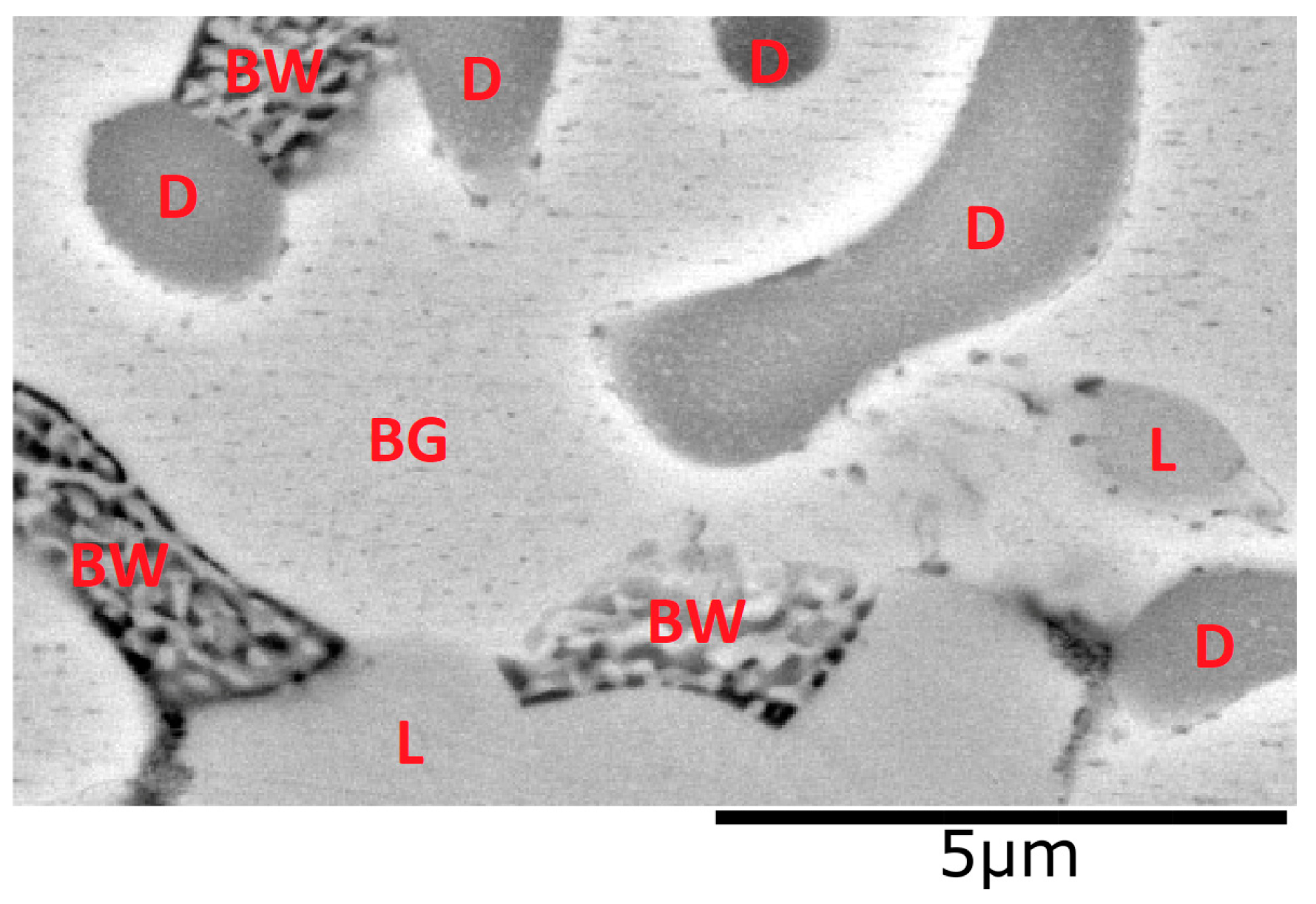
| 1 | η(Zn) | solid solution | BG background |
| 2 | η(Zn) + α(Al) | eutectoid (mixture of the solid solutions) | BW black and white |
| 3 | Mg2Zn11 | intermetallic phase | L light |
| 4 | Mg2Sn | intermetallic phase | D dark |
| Sn [%] | Description |
|---|---|
| 0 | noise 0.05~0.08, contrast BG/L 0.1 [25.5 pixels] background rel. horizontal, multiple backgrounds unobserved white rim up to 0.08 amplitude in BG on the borders L shapes: rel. narrow and long, horizontal bottom + drift some background precipitates remained after noise removal BW shapes: texture with regular alternation of B and W |
| 1 | noise 0.05~0.08, contrast BG/L 0.05 [13 pixels] multiple backgrounds possible (drift from 3 to 5 pixels across the entire image) white rim up to 0.15 amplitude in BG on the borders with: BW, D, and another BG L shapes: wider and more oval D shapes: area smaller than L shapes, intensity value varies possible presence of D shapes with high-intensity interior, which are much larger in area essentially no background precipitates after noise removal BW shapes: texture with regular alternation of B and W; pure black; irregular texture |
| 2 | noise 0.05~0.08, contrast BG/L 0.08 [20 pixels] rarely multiple backgrounds (drift from 5 to 15 pixels across the entire image) white rim up to 0.2 amplitude in BG on the borders with: BW and D D shapes: area smaller than L shapes, intensity value varies rare presence of D shapes with high-intensity interior, which are much larger in area essentially no background precipitates after noise removal BW shapes: texture more regular than at 1% Sn but less than at 0% Sn |
| 3 | noise 0.05~0.08, contrast BG/L 0.05 [13 pixels] background rel. horizontal, multiple backgrounds unobserved white rim up to 0.2 amplitude in BG on the borders with: BW and D D shapes: area larger than at 1% Sn and 2% Sn, intensity value varies essentially no background precipitates after noise removal BW shapes: texture rel. regular like at 0% Sn; rarely pure black |
| Figure 7 | Running Times | Information | |
|---|---|---|---|
| preprocessing | block 1 | 7 [ms] | im2gray, im2single |
| noise filter (Zoom4000) | block 2 | 60 [s] | 3× NLM filter |
| technical filter | blocks 7,8,9,10 | 0.4 [s] | 1× repetition |
| block 11 | 20 [s] |
| Matlab Functions | Running Time | |
|---|---|---|
| 1 | fitdist + pdf | 1.5 [s] |
| 2 | histcounts + conv | 4 [ms] |
| Sn | Zoom4000 | Zoom2000 | Zoom1000 | |||
|---|---|---|---|---|---|---|
[%] | PQ [%] | Accuracy [%] | PQ [%] | Accuracy [%] | PQ [%] | Accuracy [%] |
| 0 | BG: 67.57 BW: 4.67 L: 27.76 | 99 | BG: 65.43 BW: 4.38 L: 30.19 | 98 | BG: 66.89 BW: 4.05 L: 29.06 | 98 |
| 1 | BG: 71.50 BW: 6.05 L: 14.44 D: 8.01 | 92 | BG: 69.21 BW: 3.59 L: 16.82 D: 10.38 | 85 | BG: 73.54 BW: 3.32 L: 15.95 D: 7.19 | 91 |
| 2 | BG: 76.76 BW: 5.40 L: 9.59 D: 8.25 | 95 | BG: 71.00 BW: 3.27 L: 17.51 D: 8.22 | 95 | BG: 70.94 BW: 3.25 L: 13.59 D: 12.22 | 82 |
| 3 | BG: 73.66 BW: 3.87 L: 9.99 D: 12.48 | 95 | BG: 80.03 BW: 4.73 L: 4.63 D: 10.61 | 93 | BG: 79.63 BW: 5.50 L: 4.30 D: 10.57 | 95 |
| Sn [%] | Images | PQ ± Std.Dev [%] | XRD ± Std.Dev [%] |
|---|---|---|---|
| 0 | 45 | BG: 66.01 ± 2.01 | BG: 66.30 ± 1.50 |
| BW: 3.37 ± 0.95 | BW: 5.50 ± 0.40 | ||
| L: 30.62 ± 2.23 | L: 28.30 ± 0.50 | ||
| Accuracy: 98.12 ± 0.74 | |||
| 1 | 45 | BG: 72.31 ± 3.78 | BG: 73.10 ± 1.00 |
| BW: 3.16 ± 0.82 | BW: 4.90 ± 0.10 | ||
| L: 19.19 ± 3.52 | L: 19.20 ± 0.20 | ||
| D: 5.34 ± 1.40 | D: 2.80 ± 0.30 | ||
| Accuracy: 95.43 ± 3.64 | |||
| 2 | 45 | BG: 75.58 ± 4.17 | BG: 78.90 ± 1.80 |
| BW: 3.29 ± 0.69 | BW: 5.00 ± 0.10 | ||
| L: 12.93 ± 4.60 | L: 11.80 ± 0.60 | ||
| D: 8.21 ± 1.50 | D: 4.30 ± 0.50 | ||
| Accuracy: 95.22 ± 3.39 | |||
| 3 | 45 | BG: 78.93 ± 2.63 | BG: 83.60 ± 2.00 |
| BW: 5.20 ± 1.08 | BW: 4.20 ± 0.50 | ||
| L: 7.05 ± 1.65 | L: 5.30 ± 1.10 | ||
| D: 8.82 ± 1.64 | D: 6.90 ± 0.80 | ||
| Accuracy: 95.56 ± 1.94 |
| Factor | Manifestation | Attribute | Operator | |
|---|---|---|---|---|
| 1 | material drift | segment horizontality | objective | |
| 2 | grain orientation (channelling) | multiple backgrounds | objective | |
| 3 | spatial representation | number, form and intensity of the shapes | objective | |
| 4 | Sn content | contrast differences | objective | informed |
| 5 | application of filters | noise removal, segment horizontality | determines | |
| 6 | microscopy parameters | noise character, brightness, contrast | determines |
| Zoom | Typical Characteristics of a Histogram | Human Readability of Threshold |
|---|---|---|
| 1000 | practically unimodal | problematic |
| 2000 | 1, 2 or 3 modes, often non-Gaussian | |
| 4000 | mainly 2 modes, sometimes 3 modes | easy |
Disclaimer/Publisher’s Note: The statements, opinions and data contained in all publications are solely those of the individual author(s) and contributor(s) and not of MDPI and/or the editor(s). MDPI and/or the editor(s) disclaim responsibility for any injury to people or property resulting from any ideas, methods, instructions or products referred to in the content. |
© 2023 by the authors. Licensee MDPI, Basel, Switzerland. This article is an open access article distributed under the terms and conditions of the Creative Commons Attribution (CC BY) license (https://creativecommons.org/licenses/by/4.0/).
Share and Cite
Kuchar, D.; Gogola, P.; Gabalcova, Z.; Nemethova, A.; Nemeth, M. Segmentation and Classification of Zn-Al-Mg-Sn SEM BSE Microstructure. Appl. Sci. 2023, 13, 1045. https://doi.org/10.3390/app13021045
Kuchar D, Gogola P, Gabalcova Z, Nemethova A, Nemeth M. Segmentation and Classification of Zn-Al-Mg-Sn SEM BSE Microstructure. Applied Sciences. 2023; 13(2):1045. https://doi.org/10.3390/app13021045
Chicago/Turabian StyleKuchar, Daniel, Peter Gogola, Zuzana Gabalcova, Andrea Nemethova, and Martin Nemeth. 2023. "Segmentation and Classification of Zn-Al-Mg-Sn SEM BSE Microstructure" Applied Sciences 13, no. 2: 1045. https://doi.org/10.3390/app13021045