
Efficient Data Transfer by Evaluating Closeness Centrality for Dynamic Social Complex Network-Inspired Routing

Abstract
:1. Introduction
2. Model and Method
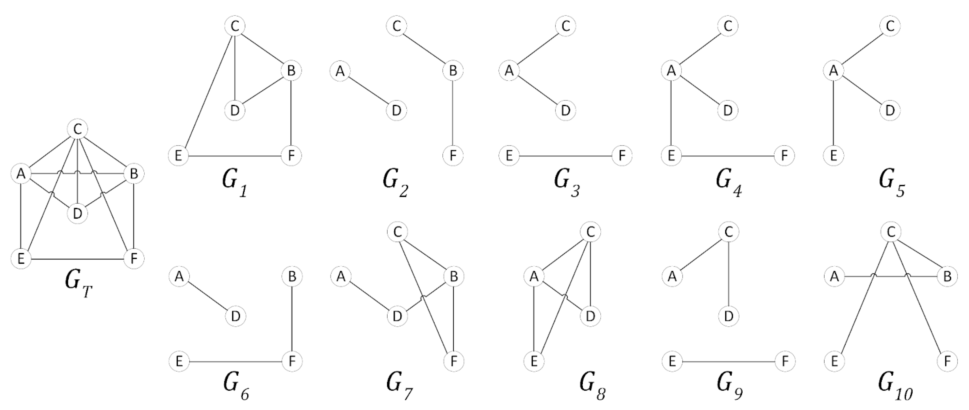
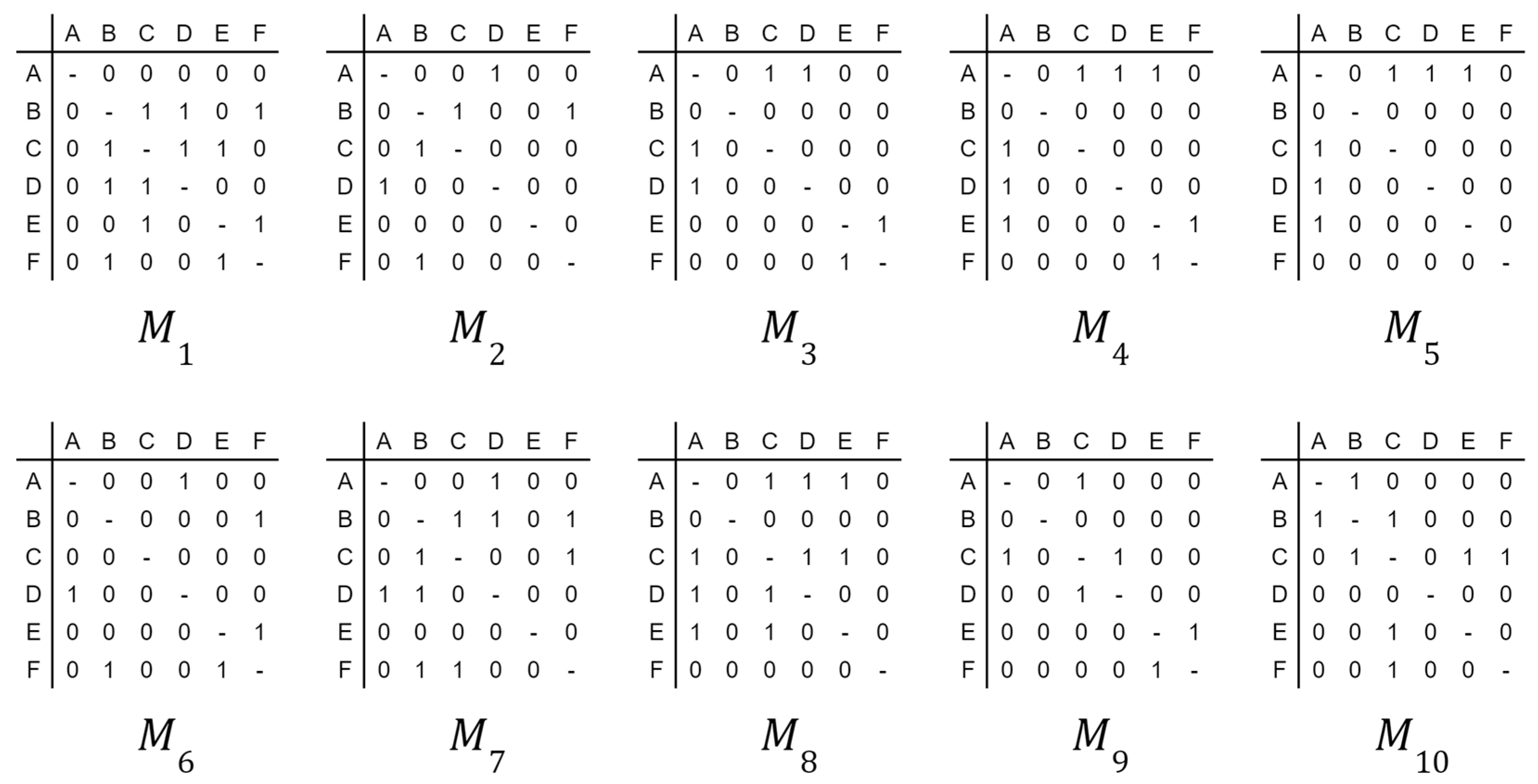
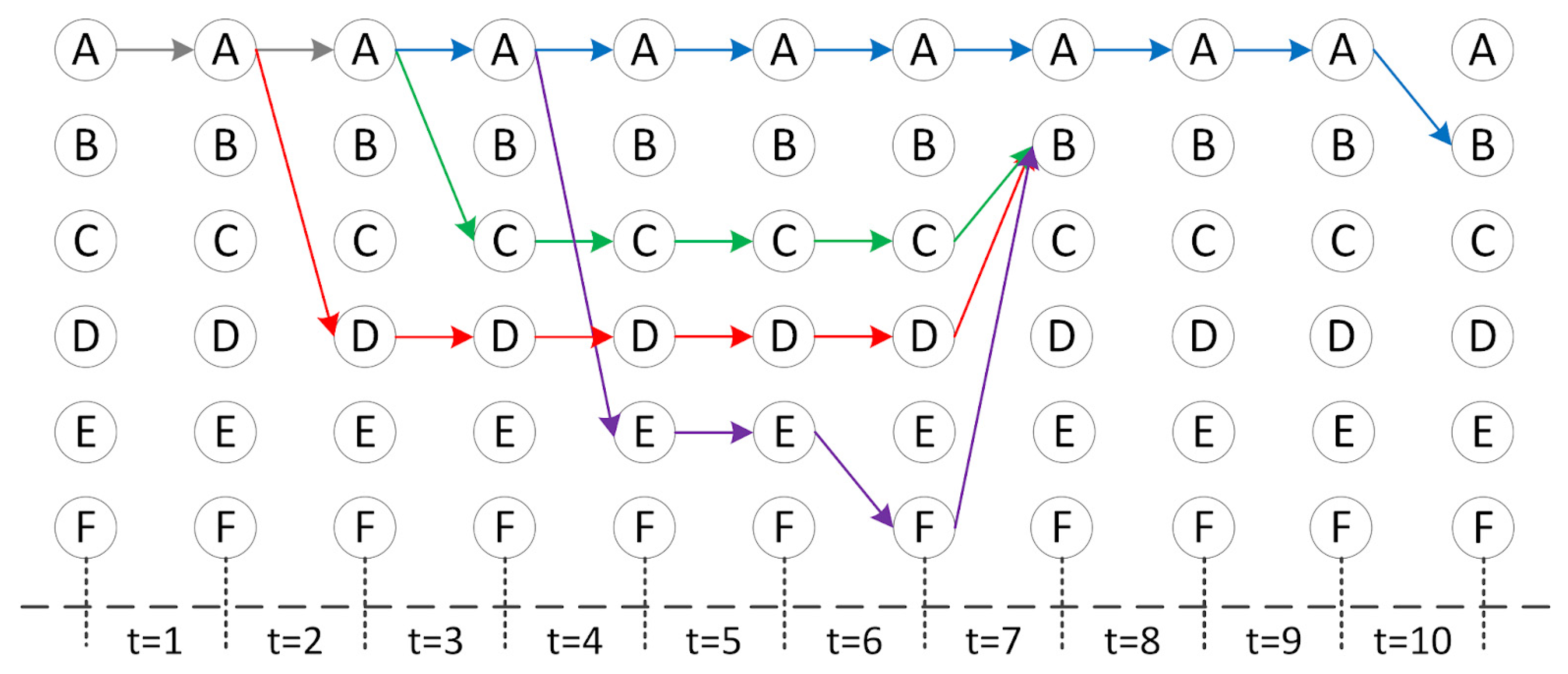
Dynamic Model of a Complex Network
- where
- represents the forwarding delay from device i to device j.
- represents the message size.
- if devices contact at any time and that link is used in a route between the source device s and the destination d (i.e., device i decides to forward a copy of the message to device j).
- if devices do not connect or if the link is not used in any route between the source device s and destination d.
- represents the encounter time of device i and device j.
- -
- Delivery Delay:
- -
- Load Balancing:
- -
- Communication Overhead:
- (the shortest path only uses one link from the source device).
- (the shortest path only uses one link to the destination device).
- (in the shortest path, if a link arriving at device k is used, then a single link leaving k will be used).
- (represents the connections of intermediary devices based on the time order).
- -
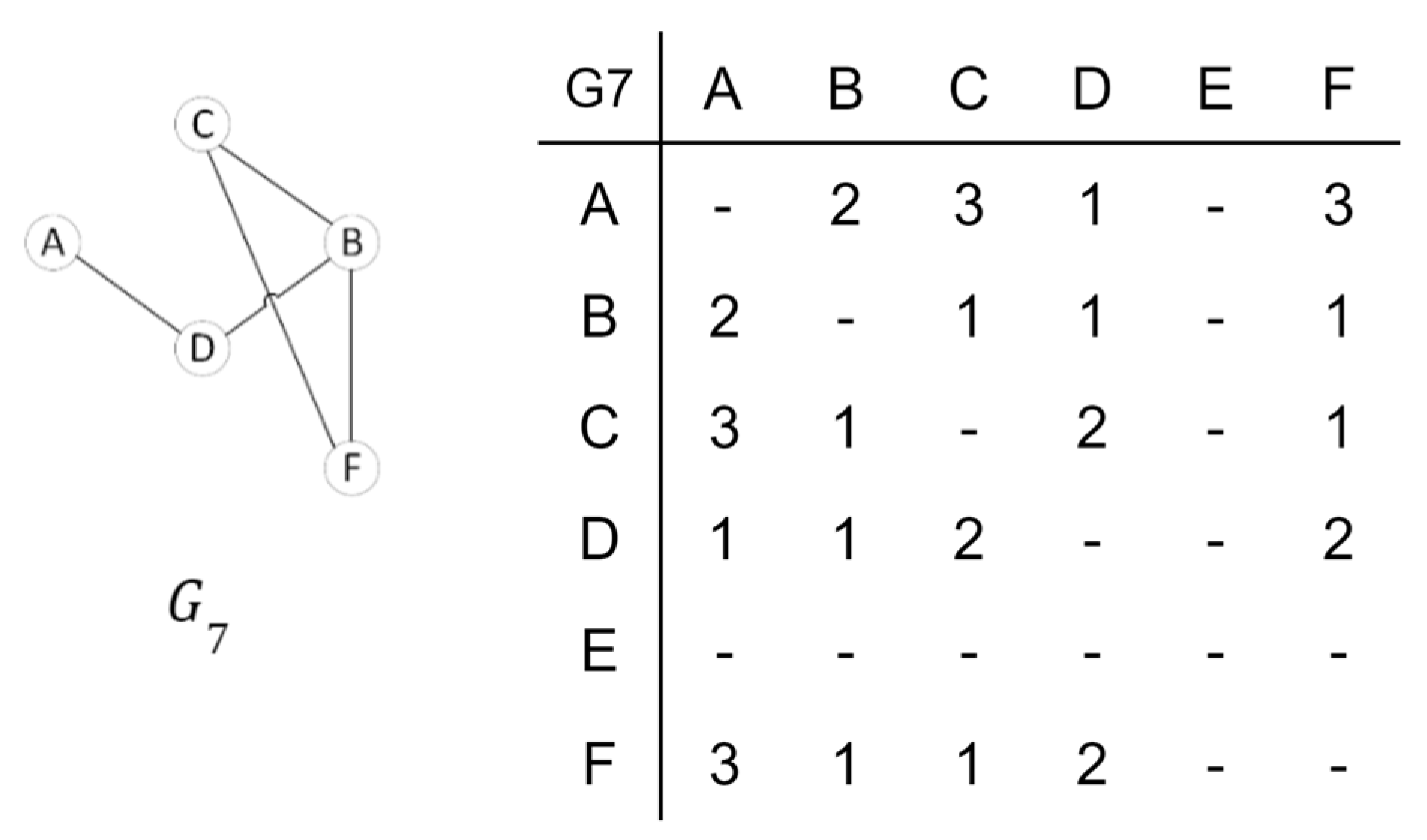
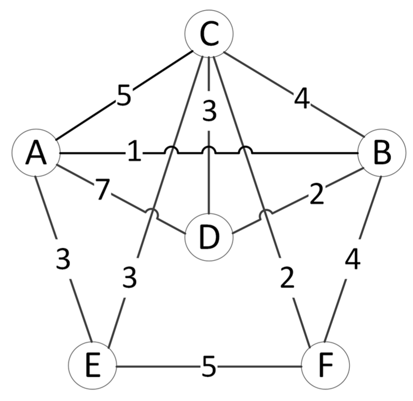
- Number of Paths between devices A and B is .
- -
- Delay matrix:
- -
- Load balancing (LB):
- -
- Load matrix:
3. Influence Metrics
3.1. Local Influence
- If it is an unweighted and undirected network,
- 2.
- If it is a weighted and undirected network,
- is the cost of the link (i, j).
- if and only if nodes i and j are connected; otherwise.
Dynamic Degree Metric
3.2. Global Influence
3.2.1. Dynamic Closeness Metric
3.2.2. Social Closeness Metric
4. Results and Discussion
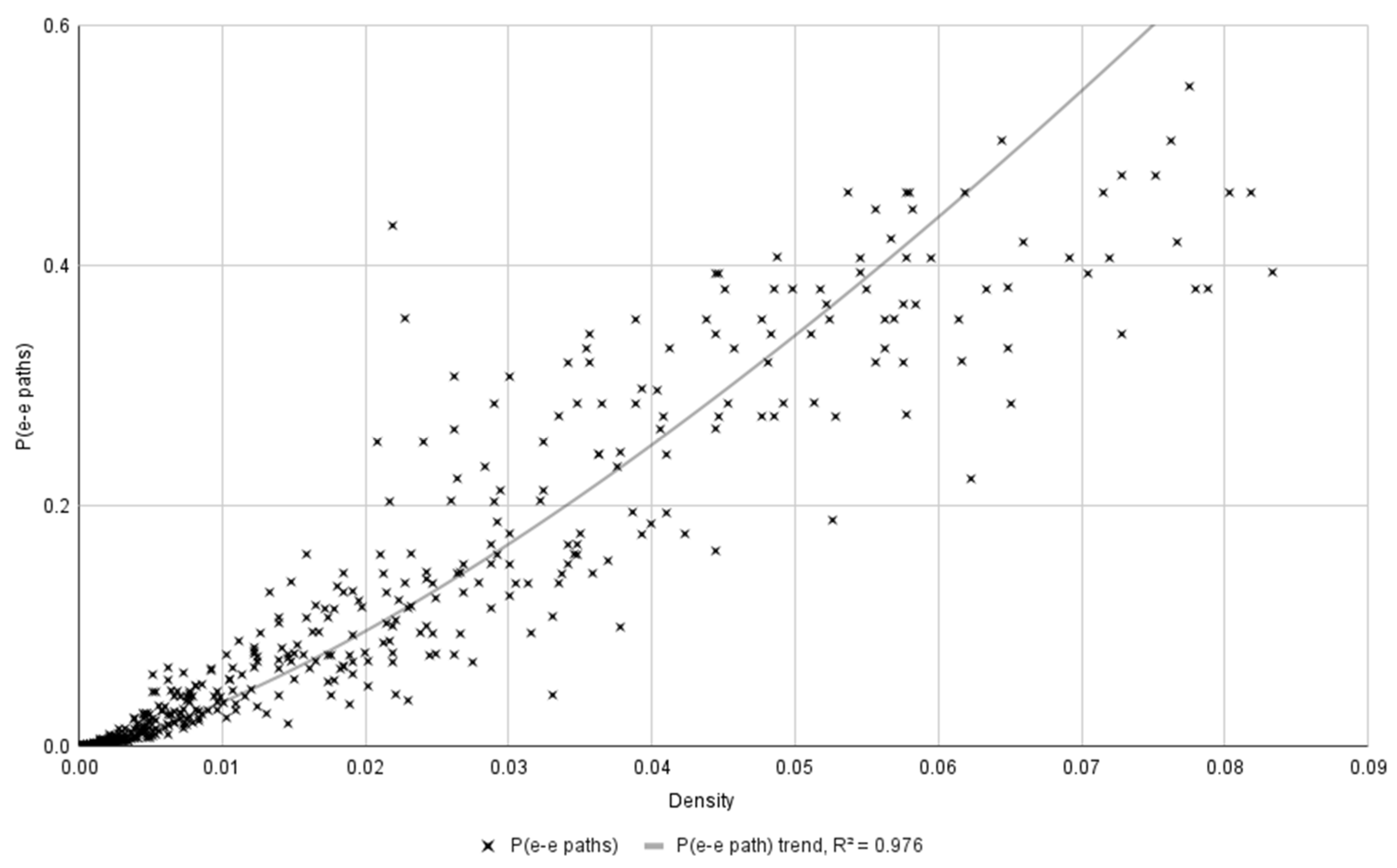
4.1. Network Density
4.2. Effectiveness Analysis of the Proposed Metrics
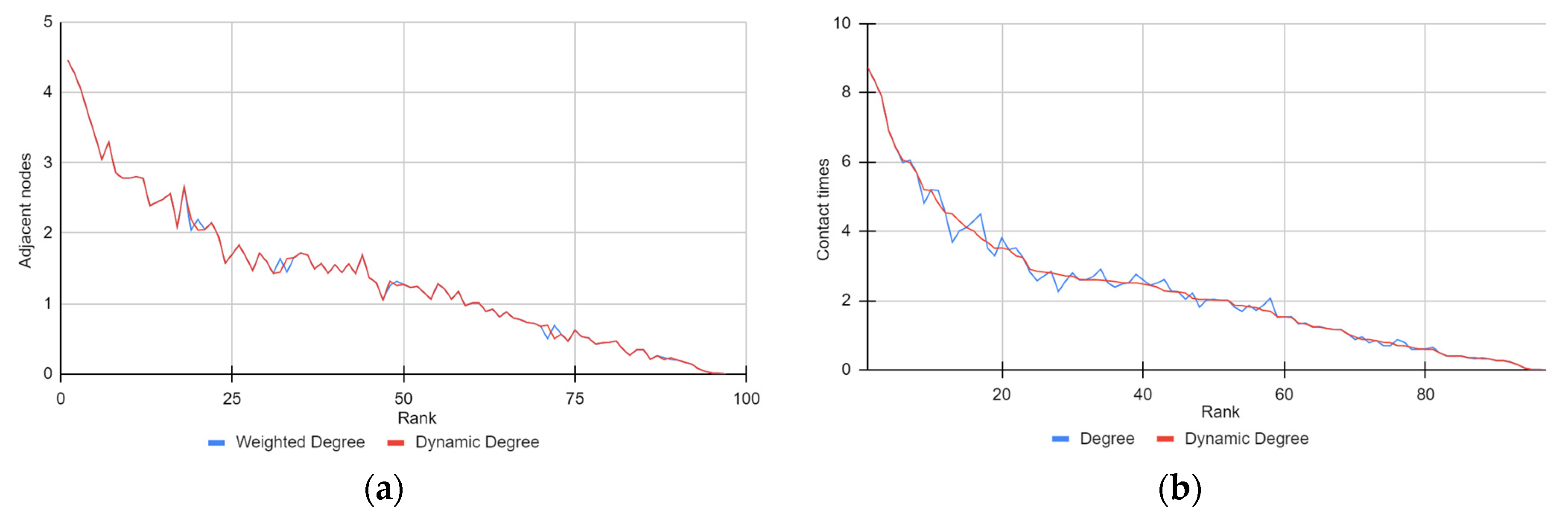
4.2.1. Local Metrics
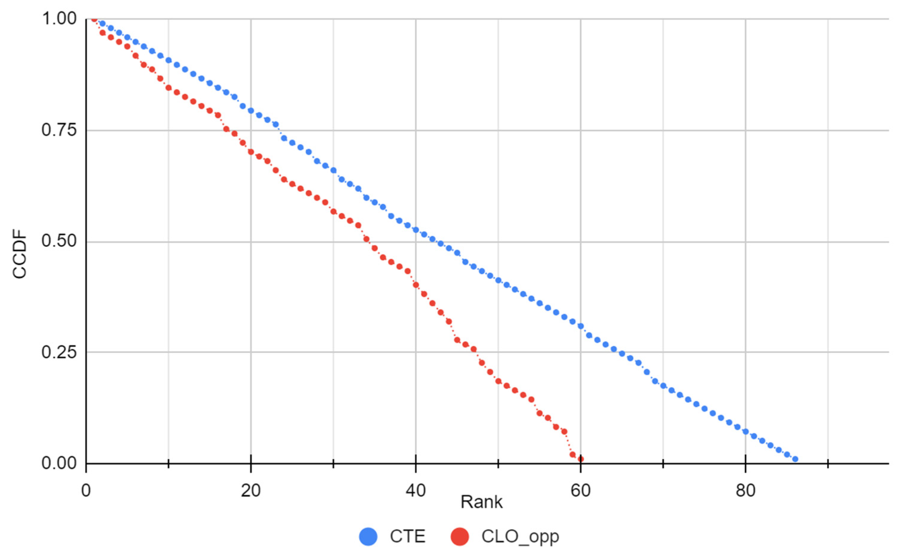
4.2.2. Global Metrics
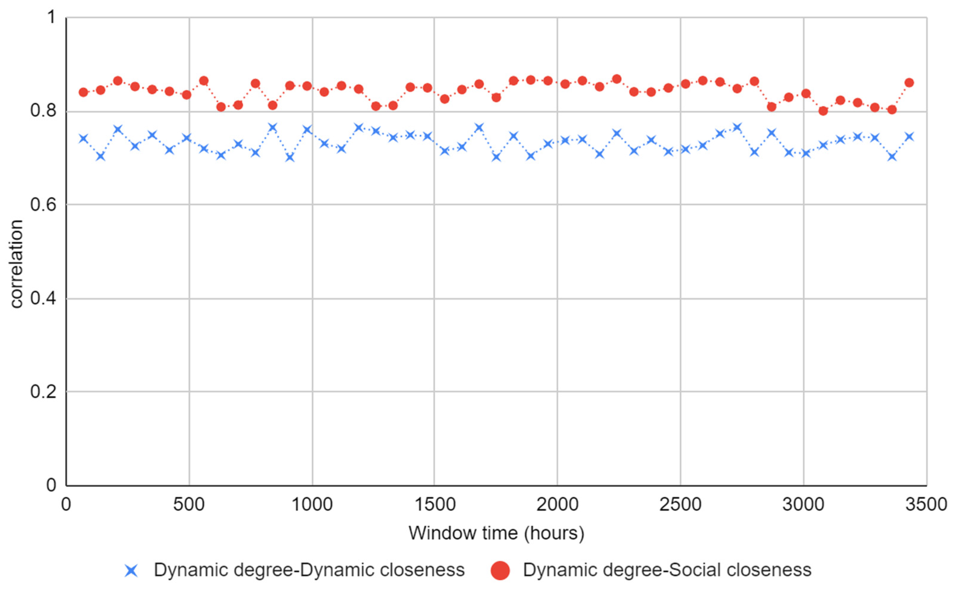
4.2.3. Correlation Analysis between Local and Global Metrics
- As one variable increases, the value of the other variable decreases; or
- Conversely, as one variable increases, the value of the other variable also increases.
- ρ represents the application of the Pearson correlation coefficient to the rank-transformed variables.
- is the covariance of the rank variables.
- and represent the standard deviations of the rank-transformed variables.
4.3. Quality of Service Metrics Analysis
4.3.1. Updating Training Matrix on Contact
| Algorithm 1. Updating training matrix on contact | |||
| Input: TM (Training Matrix), N1 and N2 (new contact between two nodes) | |||
| Output: TM (a new version of Training Matrix) | |||
| 1 | begin | ||
| 2 | if TM[N1, N2] == null then | ||
| 3 | TM[N1, N2] = 0; | ||
| 4 | if TM[N2, N1] == null then | ||
| 5 | TM[N2, N1] = 0; TM[N1, N2] +=1; | ||
| 6 | TM[N1, N2] +=1; | ||
| 7 | TM[N1, N2] +=1; | ||
| 8 | return TM | ||
4.3.2. Calculation of Friends Nodes upon Contact
| Algorithm 2. Calculation of Friend Nodes on contact | ||||
| Input: N1 LNF (List of N1 friends), N1 and N2 (new contact between two nodes) | ||||
| Output: N1 LNF (a new version of N1 friends), T(N1,N2) (timeout between N1 and N2) and TL(N1,N2) (temporal locality between L1 and L2) | ||||
| 1 | begin | |||
| 2 | MAX_TIMEOUT = 20,000; | |||
| 3 | if N2 in N1 LNF then | |||
| 4 | elapsed_time = (current_time − T(N1,N2)); | |||
| 5 | if elapsed_time < MAX_TIMEOUT then | |||
| 6 | TL(N1, N2) +=1; | |||
| 7 | else | |||
| 8 | add N2 to N1 LNF; | |||
| 9 | T(N1, N2) = current_time; | |||
| 10 | return N1 LNF, T(N1,N2), TL(N1,N2) | |||
| 11 | repeat with the input: N2 LNF, N1 and N2 | |||
4.3.3. Routing Decision on Contact
| Algorithm 3. Routing decision on contact | ||||
| Input: N1 and N2 (new contact between two nodes), R (best nodes ranking), N1 LNF | ||||
| Output: N2 messages queue | ||||
| 1 | begin | |||
| 2 | for each message in N1 queue do | |||
| 3 | N3 = obtain message destination; | |||
| 4 | is_one_of_best_nodes = (N2 in R); | |||
| 5 | are_friends = (N3 in N1 LNF); | |||
| 6 | arrived_to_destination = (N2 == N3); | |||
| 7 | if is_one_of_best_nodes or are_friends or arrived_to_destination then | |||
| 8 | forward message to N2 queue; | |||
| 9 | end for | |||
| 10 | return N2 messages queue | |||
- Node B ranks among the top positions in the ranking obtained through Algorithm 1. Being a node with good connectivity, it is more likely to successfully deliver the packet to the intended recipient or another node that can assist in reaching the message’s destination;
- The source and destination nodes of the message are friends. This indicates that they have previously connected and are likely to reconnect. Therefore, node A, carrying the message, is allowed to deliver a copy to node B;
- Node B is the intended destination of the message. In this scenario, it is logical for node A to deliver the message to node B.
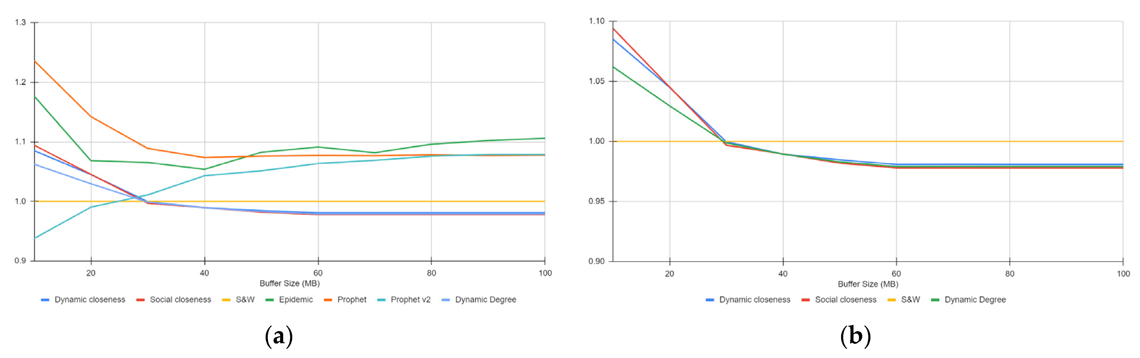
4.3.4. Packet Latency
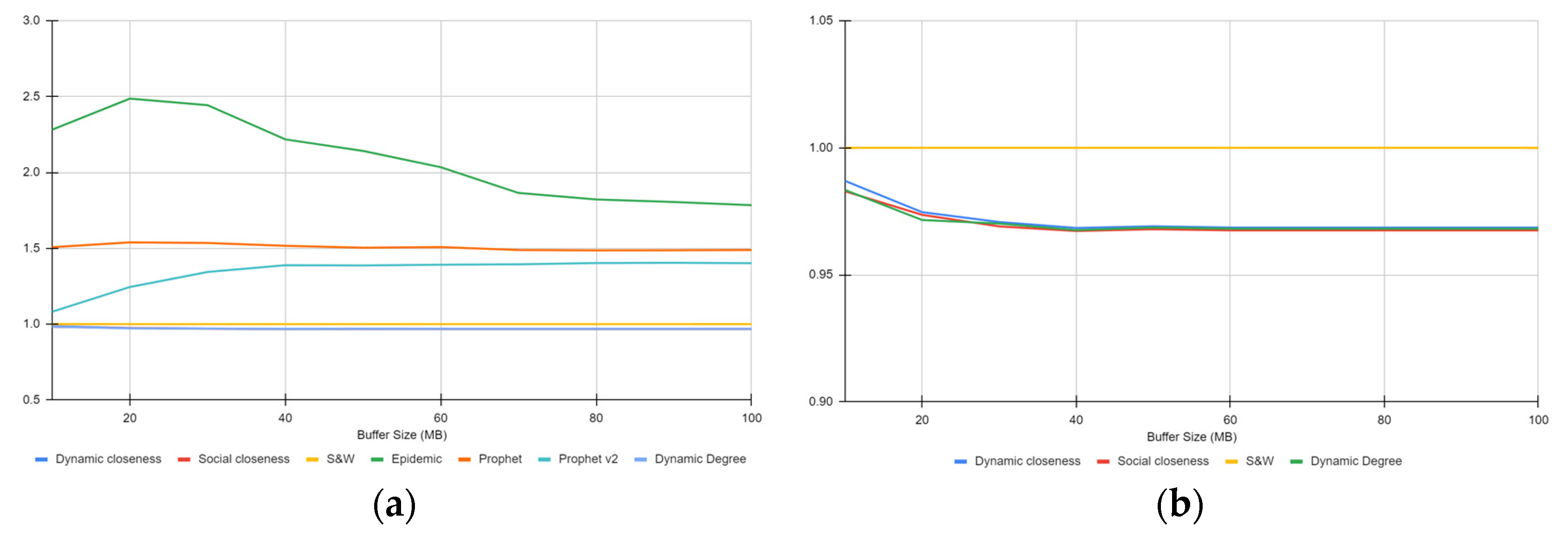
4.3.5. Path Length
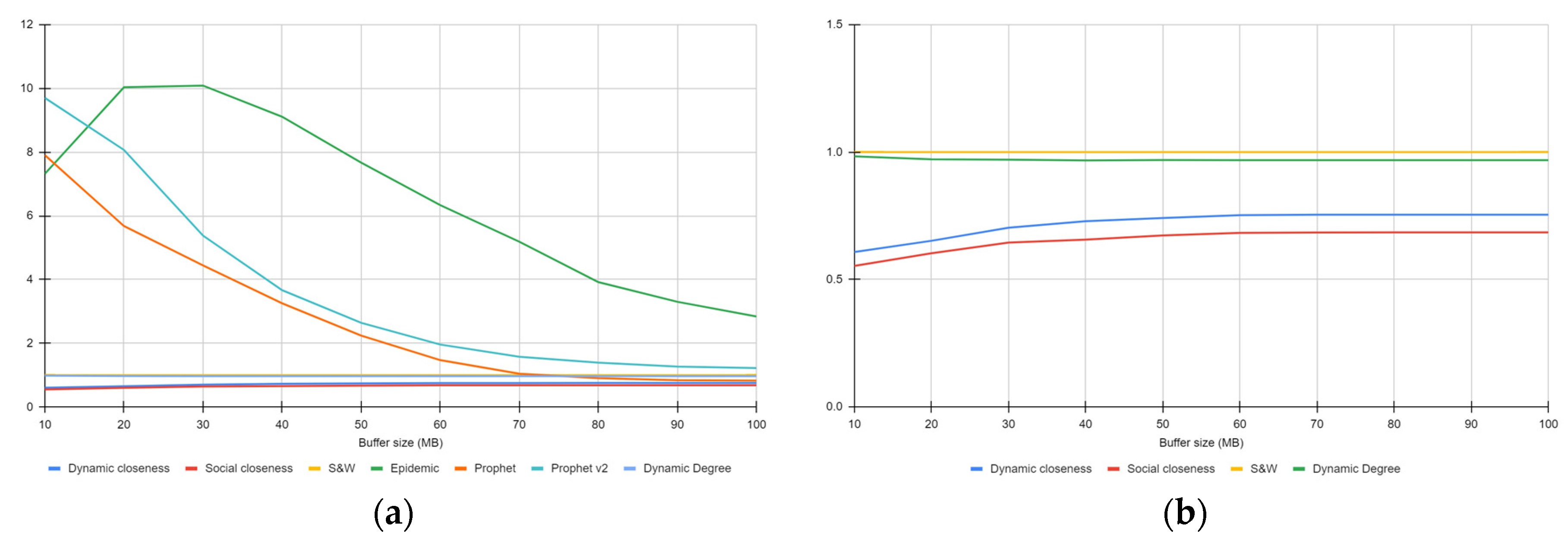
4.3.6. Route Overhead
4.3.7. Discussion of the Results
5. Conclusions and Future Work
Author Contributions
Funding
Institutional Review Board Statement
Informed Consent Statement
Data Availability Statement
Conflicts of Interest
Appendix A


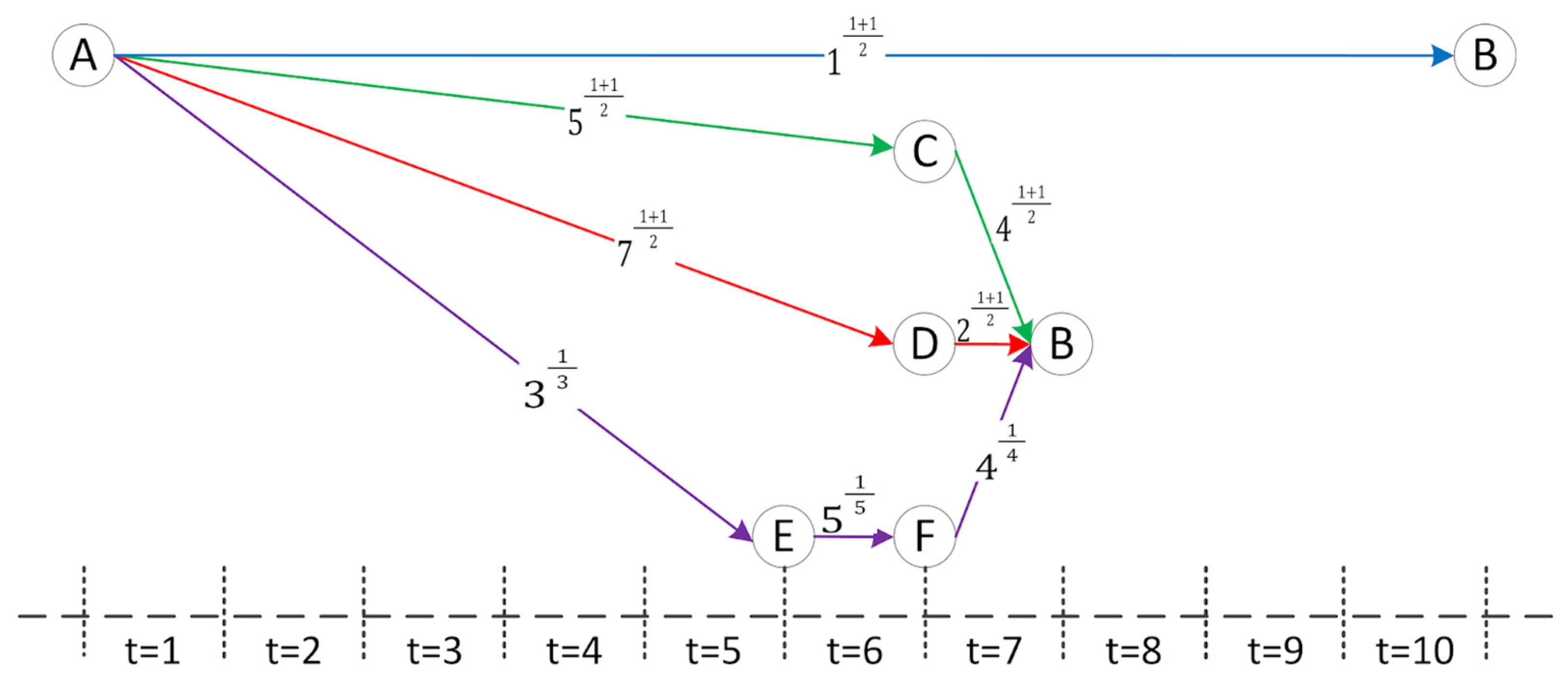
| Path | Latency | Load Balancing | Overhead | ORIT | ORIT Balancing | Costopp |
|---|---|---|---|---|---|---|
| {A, B} | 10t | 0t | 2λ | 0 | 1 | |
| {A, C, B} | 7t | 0.5t | 3λ | , | 4.5 | 0.5226 |
| {A, D, B} | 7t | 1.t | 3λ | , | 4.5 | 1.0437 |
| {A, E, F, B} | 7t | 1.5764t | 4λ | ,, | 1.5087 | 2.1408 |
References
- Number of Smartphone Mobile Network Subscriptions Worldwide from 2016 to 2022, with Forecasts from 2023 to 2028. Available online: https://www.statista.com/statistics/330695/number-of-smartphone-users-worldwide/ (accessed on 30 June 2023).
- Zhang, H.; Chen, Z.; Wu, J.; Liu, K. FRRF: A Fuzzy Reasoning Routing-Forwarding Algorithm Using Mobile Device Similarity in Mobile Edge Computing-Based Opportunistic Mobile Social Networks. IEEE Access 2019, 7, 35874–35889. [Google Scholar] [CrossRef]
- Gantha, S.S.; Jaiswal, S.; Ppallan, J.M.; Arunachalam, K. Path Aware Transport Layer Solution for Mobile Networks. IEEE Access 2020, 8, 174605–174613. [Google Scholar] [CrossRef]
- Yuan, X.; Yao, H.; Wang, J.; Mai, T.; Guizani, M. Artificial Intelligence Empowered QoS-Oriented Network Association for Next-Generation Mobile Networks. IEEE Trans. Cogn. Commun. Netw. 2021, 7, 856–870. [Google Scholar] [CrossRef]
- He, B.; Wang, J.; Qi, Q.; Sun, H.; Liao, J. RTHop: Real-Time Hop-by-Hop Mobile Network Routing by Decentralized Learning with Semantic Attention. IEEE Trans. Mob. Comput. 2023, 22, 1731–1747. [Google Scholar] [CrossRef]
- Soelistijanto, B.; Howarth, M.P.; Qi, Q.; Sun, H.; Liao, J. Transfer Reliability and Congestion Control Strategies in Opportunistic Networks: A Survey. IEEE Commun. Surv. Tutor. 2014, 16, 538–555. [Google Scholar] [CrossRef]
- Xiong, F.; Xia, L.; Xie, J.; Sun, H.; Wang, H.; Li, A.; Yu, Y. Is Hop-by-Hop Always Better Than Store-Carry-Forward for UAV Network? IEEE Access 2019, 7, 154209–154223. [Google Scholar] [CrossRef]
- Anh Duong, D.V.; Kim, D.Y.; Yoon, S. TSIRP: A Temporal Social Interactions-Based Routing Protocol in Opportunistic Mobile Social Networks. IEEE Access 2021, 9, 72712–72729. [Google Scholar] [CrossRef]
- Hajarathaiah, K.; Enduri, M.K.; Dhuli, S.; Anamalamudi, S.; Cenkeramaddi, L.R. Generalization of Relative Change in a Centrality Measure to Identify Vital Nodes in Complex Networks. IEEE Access 2023, 11, 808–824. [Google Scholar] [CrossRef]
- Qiu, L.; Zhang, J.; Tian, X.; Zhang, S. Identifying Influential Nodes in Complex Networks Based on Neighborhood Entropy Centrality. Comput. J. 2021, 64, 1465–1476. [Google Scholar] [CrossRef]
- Ibrahim, M.H.; Missaoui, R.; Vaillancourt, J. Cross-Face Centrality: A New Measure for Identifying Key Nodes in Networks Based on Formal Concept Analysis. IEEE Access 2020, 8, 206901–206913. [Google Scholar] [CrossRef]
- Zhu, Y.; Ma, H. Ranking Hubs in Weighted Networks with Node Centrality and Statistics. In Proceedings of the Fifth International Conference on Instrumentation and Measurement, Computer, Communication and Control (IMCCC), Qinhuangdao, China, 18–20 September 2015. [Google Scholar]
- Liu, M.; Zeng, Y.; Jiang, Z.; Liu, Z.; Ma, J. Centrality Based Privacy Preserving for Weighted Social Networks. In Proceedings of the 13th International Conference on Computational Intelligence and Security (CIS), Hong Kong, China, 15–18 December 2017. [Google Scholar]
- Niu, J.; Fan, J.; Wang, L.; Stojinenovic, M. K-hop centrality metric for identifying influential spreaders in dynamic large-scale social networks. In Proceedings of the IEEE Global Communications Conference, Austin, TX, USA, 8–12 December 2014. [Google Scholar]
- Rogers, T. Null models for dynamic centrality in temporal networks. J. Complex Netw. 2015, 3, 113–125. [Google Scholar] [CrossRef]
- Opsahl, T.; Agneessens, F.; Skvoretz, J. Node centrality in weighted networks: Generalizing degree and shortest paths. Soc. Netw. 2010, 32, 245–251. [Google Scholar] [CrossRef]
- Kim, H.; Anderson, R. Temporal node centrality in complex networks. Phys. Rev. E 2012, 85, 026107. [Google Scholar] [CrossRef] [PubMed]
- Trajkovic, L. Complex Networks. In Proceedings of the IEEE 19th International Conference on Cognitive Informatics & Cognitive Computing (ICCI*CC), Beijing, China, 26–28 September 2020. [Google Scholar]
- Zhang, S.-S.; Liang, X.; Wei, Y.-D.; Zhang, X. On Structural Features, User Social Behavior, and Kinship Discrimination in Communication Social Networks. IEEE Trans. Comput. Soc. Syst. 2020, 7, 425–436. [Google Scholar] [CrossRef]
- Elmezain, M.; Othman, E.A.; Ibrahim, H.M. Temporal Degree-Degree and Closeness-Closeness: A New Centrality Metrics for Social Network Analysis. Mathematics 2021, 9, 2850. [Google Scholar] [CrossRef]
- Wang, Y.; Li, H.; Zhang, L.; Zhao, L.; Li, W. Identifying influential nodes in social networks: Centripetal centrality and seed exclusion approach. Chaos Solitons Fractals 2022, 162, 112513. [Google Scholar] [CrossRef]
- Caschera, M.C.; D’Ulizia, A.; Ferri, F.; Grifoni, P. MONDE: A method for predicting social network dynamics and evolution. Evol. Syst. 2019, 10, 363–379. [Google Scholar] [CrossRef]
- Ugurlu, O. Comparative analysis of centrality measures for identifying critical nodes in complex networks. J. Comput. Sci. 2022, 62, 101738. [Google Scholar] [CrossRef]
- Dey, P.; Bhattacharya, S.; Roy, S. A Survey on the Role of Centrality as Seed Nodes for Information Propagation in Large Scale Network. ACM/IMS Trans. Data Sci. 2021, 2, 1–25. [Google Scholar] [CrossRef]
- Omar, Y.M.; Plapper, P. A Survey of Information Entropy Metrics for Complex Networks. Entropy 2020, 22, 1417. [Google Scholar] [CrossRef]
- Gao, Z.; Shi, Y.; Chen, S. Measures of node centrality in mobile social networks. Int. J. Mod. Phys. C 2015, 26, 1550107. [Google Scholar] [CrossRef]
- Wei, B.; Kawakami, W.; Kanai, K.; Katto, J. A History-Based TCP Throughput Prediction Incorporating Communication Quality Features by Support Vector Regression for Mobile Network. In Proceedings of the 13th International Conference on Information and Communication Technology Convergence (ICTC), Taichung, Taiwan, 11–13 December 2017. [Google Scholar]
- Awane, H.; Ito, Y.; Koizumi, M. Study on QoS Estimation of In-vehicle Ethernet with CBS by Multiple Regression Analysis. In Proceedings of the IEEE International Symposium on Multimedia (ISM), Jeju Island, Republic of Korea, 19–21 October 2022. [Google Scholar]
- Chen, W.; Zhou, Y. A Link Prediction Similarity Index Based on Enhanced Local Path Method. In Proceedings of the 40th Chinese Control Conference (CCC), Shanghai, China, 26–28 July 2021. [Google Scholar]
- Varma, S.; Shivam, S.; Thumu, A.; Bhushanam, A.; Sarkar, D. Jaccard Based Similarity Index in Graphs: A Multi-Hop Approach. In Proceedings of the IEEE Delhi Section Conference (DELCON), New Delhi, India, 11–13 February 2022. [Google Scholar]
- Ahmad, I.; Akhtar, M.; Noor, S.; Shahnaz, A. Missing Link Prediction using Common Neighbor and Centrality based Parameterized Algorithm. Nat. Sci. Rep. 2020, 10, 364. [Google Scholar] [CrossRef] [PubMed]
- Eagle, N.; Pentland, A. Reality mining: Sensing complex social systems. Pers. Ubiquitous Comput. 2006, 10, 255–268. [Google Scholar] [CrossRef]
- Orlinski, M.; Filer, N. The rise and fall of spatio-temporal clusters in mobile ad hoc networks. Ad Hoc Netw. 2013, 11, 1641–1654. [Google Scholar] [CrossRef]
- Anulakshmi, S.; Anand, S.; Ramesh, M.V. Impact of Network Density on the Performance of Delay Tolerant Protocols in Heterogeneous Vehicular Network. In Proceedings of the International Conference on Wireless Communications Signal Processing and Networking (WiSPNET), Chennai, India, 21–23 March 2019. [Google Scholar]
- Sati, M.; Shanab, S.; Elshawesh, A.; Sati, S.O. Density and Degree Impact on Opportunistic Network Communications. In Proceedings of the IEEE 1st International Maghreb Meeting of the Conference on Sciences and Techniques of Automatic Control and Computer Engineering MI-STA, Tripoli, Libya, 25–27 May 2021. [Google Scholar]
- Dede, J.; Förster, A.; Hernández-Orallo, E.; Herrera-Tapia, J.; Kuladinithi, K.; Kuppusamy, V.; Vatandas, Z. Simulating opportunistic networks: Survey and future directions. IEEE Commun. Surv. Tutor. 2017, 20, 1547–1573. [Google Scholar] [CrossRef]
- Khan, M.; Liu, M.; Dou, W.; Yu, S. vGraph: Graph Virtualization towards Big Data. In Proceedings of the Third IEEE International Conference on Advanced Cloud and Big Data (CBD), Yangzhou, China, 30 October–1 November 2015. [Google Scholar]


| Study | Objective | Methodology | Key Findings |
|---|---|---|---|
| [20] | Detection of influential nodes in dynamic weighted networks. | Time-ordered weighted graph models with Opshal’s algorithms, considering temporal aspects. | New hybrid centrality measure: Temporal Closeness-Closeness measure. |
| [21] | Identification of influential spreaders. | Integrate degree, constraint coefficient, and k-shell for a comprehensive assessment of node importance. | Centripetal centrality as an effective measure to identify influential nodes. |
| [22] | Prediction of the dynamics and evolution of a social network. | Two-layer HMM to model individual and group dynamics. | MONDE, demonstrating prediction accuracy rates for dynamics and evolution in social networks. |
| [23] | Detection of critical nodes of networks. | Compare centrality measures’ effectiveness. | Isolating centrality as an effective measure for identifying critical nodes. |
| [24] | Correlation between seed node detection and information flow. | Investigate different centrality measures for seed node detection. | Emphasize the impact of network structure on seed node selection. |
| Title 1 | Latency | Load Balancing | Overhead |
|---|---|---|---|
| {A, B} | 10t | 0t | 2λ |
| {A, C, B} | 7t | 0.5t | 3λ |
| {A, D, B} | 7t | 1.5t | 3λ |
| {A, E, F, B} | 7t | 1.5764t | 4λ |
| Feature | Value |
|---|---|
| Number of devices | 97 |
| Environment | Campus |
| Dataset duration | 246 days |
| Dataset duration used | 196 days |
| Encounter prob. 1st 1/4 day | 0.0003 |
| Encounter prob. 2nd 1/4 day | 0.0011 |
| Encounter prob. 3rd 1/4 day | 0.0019 |
| Encounter prob. 4th 1/4 day | 0.0012 |
| Percentage of dataset duration for the Training Graph (GT) | 75% |
| Percentage of dataset duration for the Probe Graph (GP) | 25% |
| Network density | <0.5% |
| Number of contacts of the top 20 devices | 4–9 |
Disclaimer/Publisher’s Note: The statements, opinions and data contained in all publications are solely those of the individual author(s) and contributor(s) and not of MDPI and/or the editor(s). MDPI and/or the editor(s) disclaim responsibility for any injury to people or property resulting from any ideas, methods, instructions or products referred to in the content. |
© 2023 by the authors. Licensee MDPI, Basel, Switzerland. This article is an open access article distributed under the terms and conditions of the Creative Commons Attribution (CC BY) license (https://creativecommons.org/licenses/by/4.0/).
Share and Cite
López-Rourich, M.A.; Rodríguez-Pérez, F.J. Efficient Data Transfer by Evaluating Closeness Centrality for Dynamic Social Complex Network-Inspired Routing. Appl. Sci. 2023, 13, 10766. https://doi.org/10.3390/app131910766
López-Rourich MA, Rodríguez-Pérez FJ. Efficient Data Transfer by Evaluating Closeness Centrality for Dynamic Social Complex Network-Inspired Routing. Applied Sciences. 2023; 13(19):10766. https://doi.org/10.3390/app131910766
Chicago/Turabian StyleLópez-Rourich, Manuel A., and Francisco J. Rodríguez-Pérez. 2023. "Efficient Data Transfer by Evaluating Closeness Centrality for Dynamic Social Complex Network-Inspired Routing" Applied Sciences 13, no. 19: 10766. https://doi.org/10.3390/app131910766