
Uncertainty Quantification for Thermodynamic Simulations with High-Dimensional Input Spaces Using Sparse Polynomial Chaos Expansion: Retrofit of a Large Thermal Power Plant
 , ,
, ,
Abstract
:1. Introduction
- The definition of a methodology to apply advanced uncertainty quantification techniques to process modeling involving large numbers of parameters and several KPIs.
- Apply this methodology to the case of a retrofitted, large biomass CHP unit.
- Investigation of the limits of uncertainty quantification (UQ) polynomial chaos expansion (PCE) and, finally, sparse PCE.
- Investigation of the most important parameters to model both cases.
2. Materials and Methods
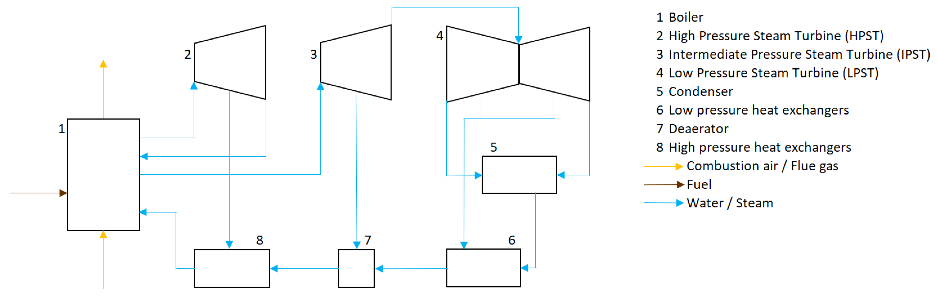
2.1. Thermodynamic Modeling and Validation
- The current situation: the fuel is coal; the power plant runs base load.
- Potential new situation: the fuel is biomass; the power plant runs at a boiler load of 80%, and there is low-temperature heat extraction in the CHP extension.
2.2. Uncertainty Characterization
2.2.1. Selection of Uncertain Input Parameters
2.2.2. Selection of Outputs
2.3. Uncertainty Quantification
2.3.1. Construction of the PCE
2.3.2. Sparse Polynomial Chaos Expansion
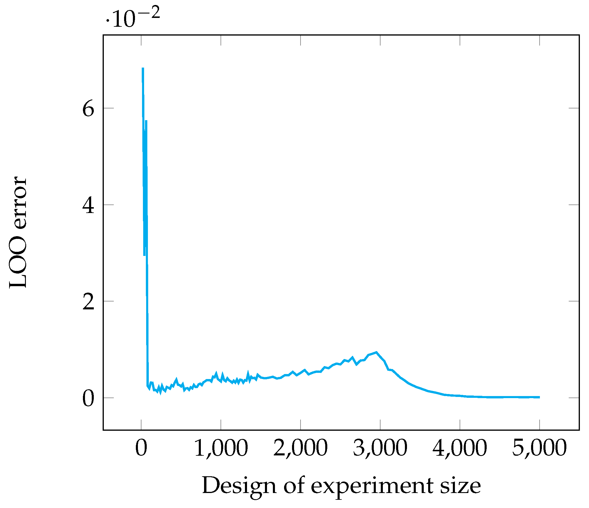
2.3.3. Error Estimation
2.3.4. Post-Processing
2.3.5. Characterization
3. Results and Discussion
3.1. General Summary of the Results
3.2. Analysis Outputs
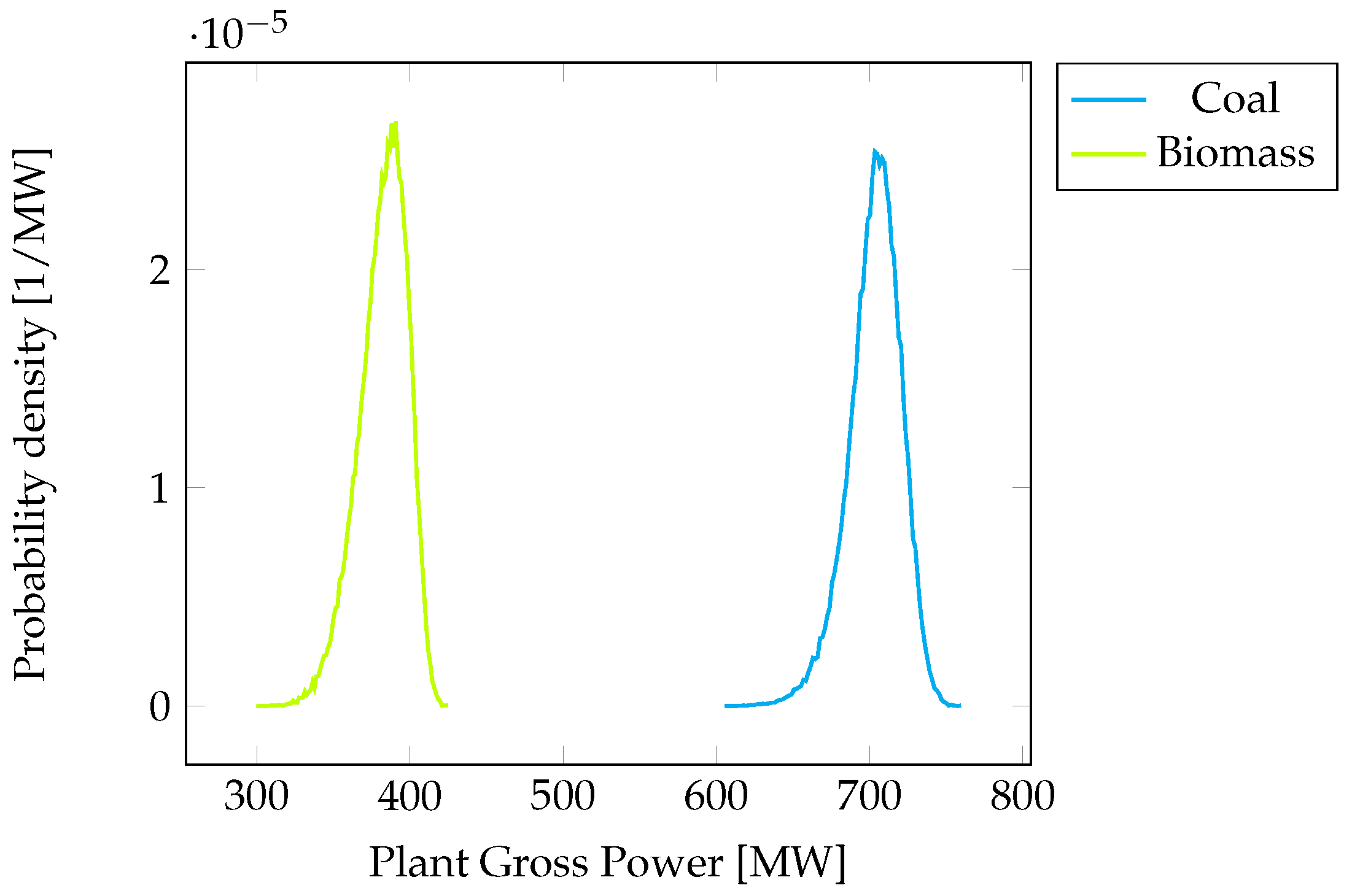
3.2.1. Plant Performance Indicators
Plant Gross Power
Plant Gross Electric Efficiency
Plant CHP Efficiency
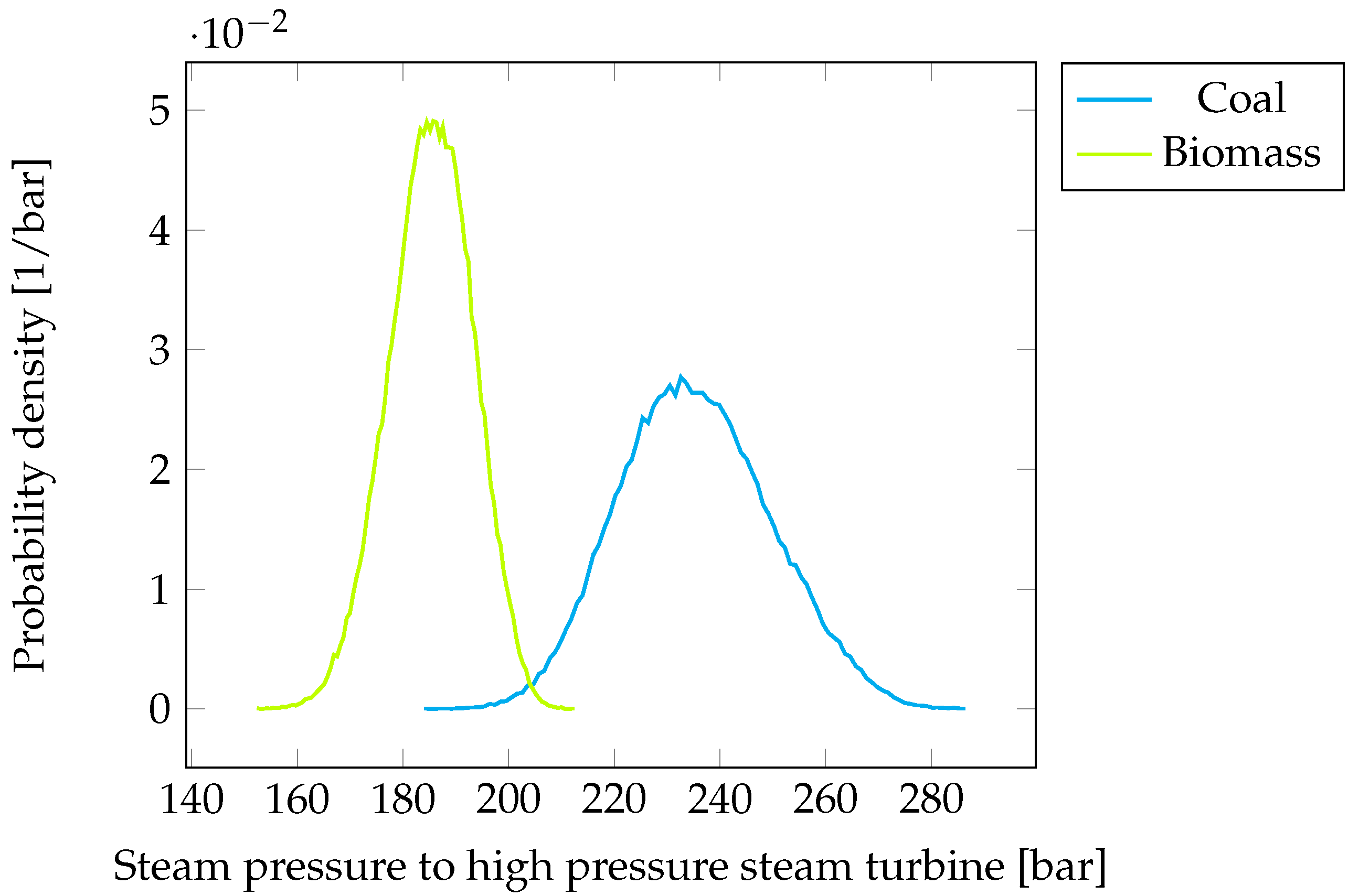
3.2.2. Steam Quality Indicators
Live Steam Pressure
Live Steam Flow Rate
3.2.3. Furnace Operation Indicators
Adiabatic Flame Temperature
Furnace Exit Gas Temperature (FEGT)
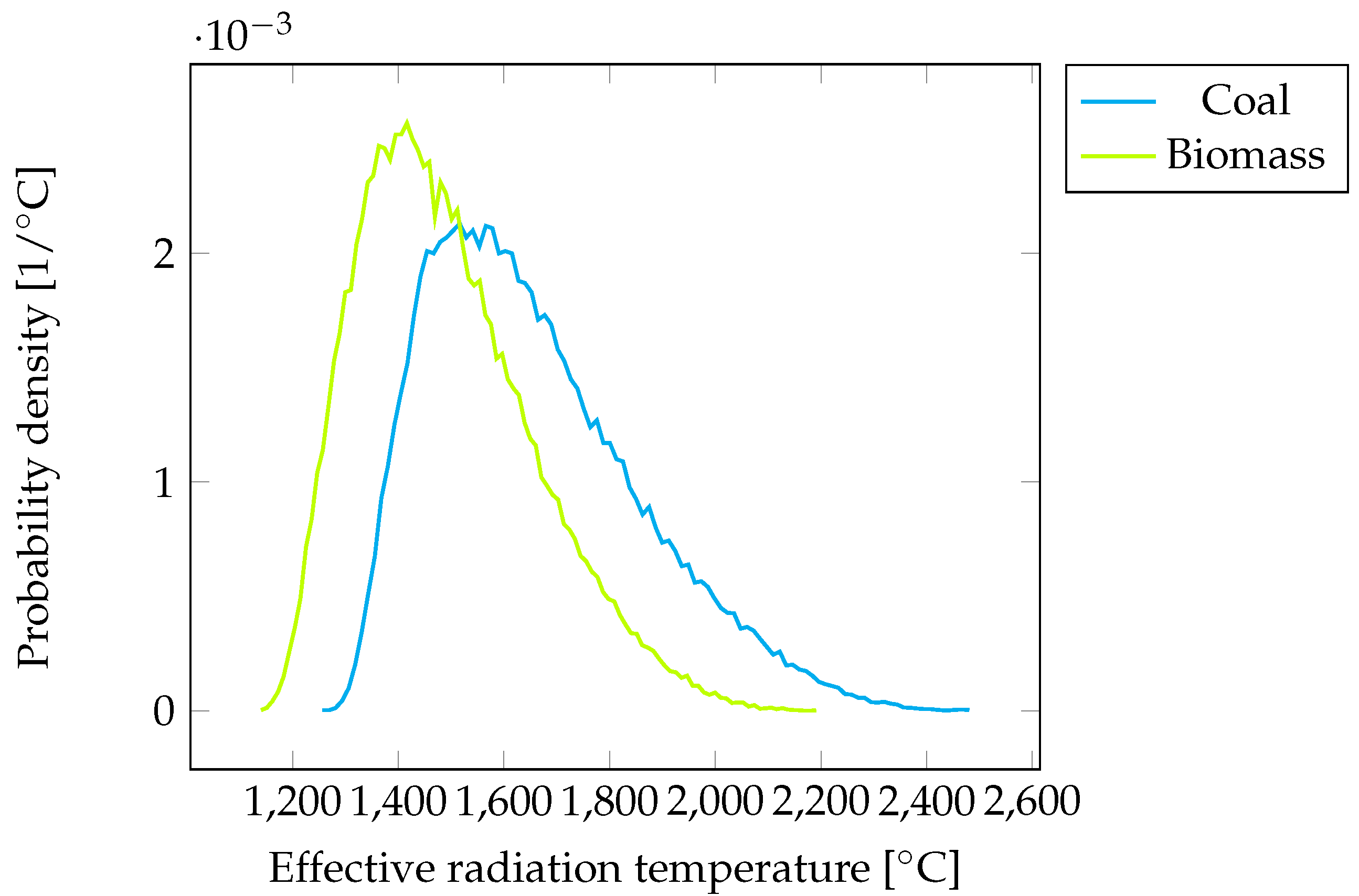
Effective Radiation Temperature
3.3. Analysis Inputs
3.3.1. Coal:
3.3.2. Biomass:
3.4. Limitations of the Study
4. Conclusions
Supplementary Materials
Author Contributions
Funding
Institutional Review Board Statement
Informed Consent Statement
Data Availability Statement
Acknowledgments
Conflicts of Interest
References
- Ang, T.Z.; Salem, M.; Kamarol, M.; Das, H.S.; Nazari, M.A.; Prabaharan, N. A comprehensive study of renewable energy sources: Classifications, challenges and suggestions. Energy Strategy Rev. 2022, 43, 100939. [Google Scholar] [CrossRef]
- Ahmad, S.; Iqbal, K.; Kothari, R.; Singh, H.M.; Sari, A.; Tyagi, V. A critical overview of upstream cultivation and downstream processing of algae-based biofuels: Opportunity, technological barriers and future perspective. J. Biotechnol. 2022, 351, 74–98. [Google Scholar] [CrossRef] [PubMed]
- Hassan, M.H.; Kalam, M.A. An Overview of Biofuel as a Renewable Energy Source: Development and Challenges. Procedia Eng. 2013, 56, 39–53. [Google Scholar] [CrossRef]
- Ciriaco, A.E.; Zarrouk, S.J.; Zakeri, G. Geothermal resource and reserve assessment methodology: Overview, analysis and future directions. Renew. Sustain. Energy Rev. 2020, 119, 109515. [Google Scholar] [CrossRef]
- Ould Amrouche, S.; Rekioua, D.; Rekioua, T.; Bacha, S. Overview of energy storage in renewable energy systems. Int. J. Hydrog. Energy 2016, 41, 20914–20927. [Google Scholar] [CrossRef]
- Olabi, A.; Abdelkareem, M. Energy storage systems towards 2050. Energy 2021, 219, 119634. [Google Scholar] [CrossRef]
- Tan, Y.; Nookuea, W.; Li, H.; Thorin, E.; Yan, J. Property impacts on Carbon Capture and Storage (CCS) processes: A review. Energy Convers. Manag. 2016, 118, 204–222. [Google Scholar] [CrossRef]
- Peres, C.B.; Resende, P.M.R.; Nunes, L.J.R.; Morais, L.C.d. Advances in Carbon Capture and Use (CCU) Technologies: A Comprehensive Review and CO2 Mitigation Potential Analysis. Clean Technol. 2022, 4, 1193–1207. [Google Scholar] [CrossRef]
- Masson-Delmotte, V.; Zhai, P.; Pörtner, H.O.H.O.; Roberts, D.; Skea, J.; Shukla, P.R.; Pirani, A.; Moufouma-Okia, W.; Pidcock, R.; Connors, S.; et al. “Summary for Policymakers” in Global Warming of 1.5 °C. An IPCC Special Report on the Impacts of Global Warming of 1.5 °C above Pre-Industrial Levels and Related Global Greenhouse Gas Emission Pathways, in the Context of Strengthening the Global Response to the Threat of Climate Change, Sustainable Development, and Efforts to Eradicate Poverty. In Sustainable Development, and Efforts to Eradicate Poverty; Technical Report; IPCC: Geneva, Switzerland, 2018. [Google Scholar]
- Halkos, G.E.; Gkampoura, E.C. Reviewing Usage, Potentials, and Limitations of Renewable Energy Sources. Energies 2020, 13, 2906. [Google Scholar] [CrossRef]
- Chiari, L.; Zecca, A. Constraints of fossil fuels depletion on global warming projections. Energy Policy 2011, 39, 5026–5034. [Google Scholar] [CrossRef]
- Global Energy Monitor. Global Coal Plant Tracker. Available online: www.globalenergymonitor.org (accessed on 22 March 2023).
- Bilgili, F.; Koçak, E.; Bulut, Ü.; Kuşkaya, S. Can biomass energy be an efficient policy tool for sustainable development? Renew. Sustain. Energy Rev. 2017, 71, 830–845. [Google Scholar] [CrossRef]
- Sebastián, F.; Royo, J.; Gómez, M. Cofiring versus biomass-fired power plants: GHG (Greenhouse Gases) emissions savings comparison by means of LCA (Life Cycle Assessment) methodology. Energy 2011, 36, 2029–2037. [Google Scholar] [CrossRef]
- Demirbas, A. Combustion characteristics of different biomass fuels. Prog. Energy Combust. Sci. 2004, 30, 219–230. [Google Scholar] [CrossRef]
- Akella, A.; Saini, R.; Sharma, M. Social, economical and environmental impacts of renewable energy systems. Renew. Energy 2009, 34, 390–396. [Google Scholar] [CrossRef]
- Variny, M.; Varga, A.; Rimár, M.; Janošovský, J.; Kizek, J.; Lukáč, L.; Jablonský, G.; Mierka, O. Advances in Biomass Co-Combustion with Fossil Fuels in the European Context: A Review. Processes 2021, 9, 100. [Google Scholar] [CrossRef]
- Xu, Y.; Yang, K.; Zhou, J.; Zhao, G. Coal-Biomass Co-Firing Power Generation Technology: Current Status, Challenges and Policy Implications. Sustainability 2020, 12, 3692. [Google Scholar] [CrossRef]
- Nawaz, Z.; Ali, U. Techno-economic evaluation of different operating scenarios for indigenous and imported coal blends and biomass co-firing on supercritical coal-fired power plant performance. Energy 2020, 212, 118721. [Google Scholar] [CrossRef]
- Tzelepi, V.; Zeneli, M.; Kourkoumpas, D.S.; Karampinis, E.; Gypakis, A.; Nikolopoulos, N.; Grammelis, P. Biomass Availability in Europe as an Alternative Fuel for Full Conversion of Lignite Power Plants: A Critical Review. Energies 2020, 13, 3390. [Google Scholar] [CrossRef]
- Bunn, D.W.; Redondo-Martin, J.; Muñoz-Hernandez, J.I.; Diaz-Cachinero, P. Analysis of coal conversion to biomass as a transitional technology. Renew. Energy 2019, 132, 752–760. [Google Scholar] [CrossRef]
- Keller, V.; Lyseng, B.; English, J.; Niet, T.; Palmer-Wilson, K.; Moazzen, I.; Robertson, B.; Wild, P.; Rowe, A. Coal-to-biomass retrofit in Alberta–value of forest residue bioenergy in the electricity system. Renew. Energy 2018, 125, 373–383. [Google Scholar] [CrossRef]
- De Meulenaere, R.; Maertens, T.; Sikkema, A.; Brusletto, R.; Barth, T.; Blondeau, J. Energetic and Exergetic Performances of a Retrofitted, Large-Scale, Biomass-Fired CHP Coupled to a Steam-Explosion Biomass Upgrading Plant, a Biorefinery Process and a High-Temperature Heat Network. Energies 2021, 14, 7720. [Google Scholar] [CrossRef]
- Rubinstein, R.Y.; Kroese, D.P. Simulation and the Monte Carlo Method; John Wiley & Sons: New York, NY, USA, 2016; Volume 10. [Google Scholar]
- Sudret, B. Polynomial chaos expansions and stochastic finite-element methods. In Risk and Reliability in Geotechnical Engineering; CRC Press: Boca Raton, FL, USA, 2014; Chapter 6; pp. 265–300. [Google Scholar]
- Deng, Z.; Hu, X.; Lin, X.; Che, Y.; Xu, L.; Guo, W. Data-driven state of charge estimation for lithium-ion battery packs based on Gaussian process regression. Energy 2020, 205, 118000. [Google Scholar] [CrossRef]
- Richard, B.; Cremona, C.; Adelaide, L. A response surface method based on support vector machines trained with an adaptive experimental design. Struct. Saf. 2012, 39, 14–21. [Google Scholar] [CrossRef]
- Rabitz, H.; Aliş, Ö.F. General foundations of high-dimensional model representations. J. Math. Chem. 1999, 25, 197–233. [Google Scholar] [CrossRef]
- Coppitters, D.; De Paepe, W.; Contino, F. Robust design optimization of a photovoltaic-battery-heat pump system with thermal storage under aleatory and epistemic uncertainty. Energy 2021, 229, 120692. [Google Scholar] [CrossRef]
- De Meulenaere, R.; Coppitters, D.; Maertens, T.; Contino, F.; Blondeau, J. Quantifying the impact of furnace heat transfer parameter uncertainties on the thermodynamic simulations of a biomass retrofit. Therm. Sci. Eng. Prog. 2023, 37, 101592. [Google Scholar] [CrossRef]
- Montgomery, D.C. Design and Analysis of Experiments; John Wiley & Sons: New York, NY, USA, 2014. [Google Scholar]
- Blatman, G. Adaptive Sparse Polynomial Chaos Expansions for Uncertainty Propagation and Sensitivity Analysis. Ph.D. Thesis, Université Blaise Pascal, Clermont-Ferrand, France, 2009. [Google Scholar]
- Lüthen, N.; Marelli, S.; Sudret, B. Sparse polynomial chaos expansions: Literature survey and benchmark. SIAM/ASA J. Uncertain. Quantif. 2021, 9, 593–649. [Google Scholar] [CrossRef]
- Donoho, D.L. Compressed sensing. IEEE Trans. Inf. Theory 2006, 52, 1289–1306. [Google Scholar] [CrossRef]
- Blatman, G.; Sudret, B. Adaptive sparse polynomial chaos expansion based on least angle regression. J. Comput. Phys. 2011, 230, 2345–2367. [Google Scholar] [CrossRef]
- Abraham, S.; Raisee, M.; Ghorbaniasl, G.; Contino, F.; Lacor, C. A robust and efficient stepwise regression method for building sparse polynomial chaos expansions. J. Comput. Phys. 2017, 332, 461–474. [Google Scholar] [CrossRef]
- THERMOFLEX, version 30; Thermoflow Inc.: Southborough, MA, USA, 2023. Available online: www.thermoflow.com(accessed on 30 April 2023).
- Abelha, P.; Cieplik, M.K. Evaluation of steam-exploded wood pellets storage and handling safety in a coal-designed power plant. Energy Fuels 2021, 35, 2357–2367. [Google Scholar] [CrossRef]
- Fosnacht, D.R.; Hendrickson, D.W. Use of Biomass Fuels in Global Power Generation with a Focus on Biomass Pre-Treatment; Technical Report; Natural resources research institute, University of Minnesota Duluth: Duluth, MN, USA, 2016. [Google Scholar]
- Lam, P.S. Steam Explosion of Biomass to Produce Durable Wood Pellets. Ph.D. Thesis, The University of British Columbia, Vancouver, BC, Canada, 2011. [Google Scholar]
- Løhre, C.; Underhaug, J.; Brusletto, R.; Barth, T. A Workup Protocol Combined with Direct Application of Quantitative Nuclear Magnetic Resonance Spectroscopy of Aqueous Samples from Large-Scale Steam Explosion of Biomass. ACS Omega 2021, 6, 6714–6721. [Google Scholar] [CrossRef] [PubMed]
- Blondeau, J.; Van den Auweele, J.; Alimuddin, S.; Binder, F.; Turoni, F. Online adjustment of Furnace Exit Gas Temperature field using advanced infrared pyrometry: Case study of a 1500 MWth utility boiler. Case Stud. Therm. Eng. 2020, 21, 100649. [Google Scholar] [CrossRef]
- Ozer, M.; Basha, O.M.; Stiegel, G.; Morsi, B. 7—Effect of coal nature on the gasification process. In Integrated Gasification Combined Cycle (IGCC) Technologies; Wang, T., Stiegel, G., Eds.; Woodhead Publishing: Sawston, UK, 2017; pp. 257–304. [Google Scholar]
- Miller, B.G. 4—Introduction to Coal Utilization Technologies. In Clean Coal Engineering Technology, 2nd ed.; Miller, B.G., Ed.; Butterworth-Heinemann: Oxford, UK, 2017; pp. 147–229. [Google Scholar]
- Coppitters, D.; Tsirikoglou, P.; De Paepe, W.; Kyprianidis, K.; Kalfas, A.; Contino, F. RHEIA: Robust design optimization of renewable Hydrogen and dErIved energy cArrier systems. J. Open Source Softw. 2022, 7, 4370. [Google Scholar] [CrossRef]
- Coppitters, D.; De Paepe, W.; Contino, F. Robust design optimization and stochastic performance analysis of a grid-connected photovoltaic system with battery storage and hydrogen storage. Energy 2020, 213, 118798. [Google Scholar] [CrossRef]
- Verleysen, K.; Parente, A.; Contino, F. How does a resilient, flexible ammonia process look? Robust design optimization of a Haber-Bosch process with optimal dynamic control powered by wind. Proc. Combust. Inst. 2023, 39, 5511–5520. [Google Scholar] [CrossRef]
- Liang, H.; Hua, H.; Qin, Y.; Ye, M.; Zhang, S.; Cao, J. Stochastic Optimal Energy Storage Management for Energy Routers via Compressive Sensing. IEEE Trans. Ind. Inform. 2022, 18, 2192–2202. [Google Scholar] [CrossRef]


| Extraction | Pressure [bar] | Temperature [°C] | Flow [kg/s] | Enthalpy [kJ/kg] |
|---|---|---|---|---|
| LP extraction | 278 | 44 | 3025 | |
| Return | 44 | |||
| IP extraction | 31 | 3145 | ||
| Return | 1 | 31 | ||
| HP extraction | 104 | 3180 | ||
| Return | 104 |
| # Output | Output Variable Description | Unit |
|---|---|---|
| Plant performance indicators | ||
| 1 | Plant gross power | MW |
| 2 | Plant gross electric efficiency | % |
| 3 | Plant CHP efficiency | % |
| Steam quality indicators | ||
| 4 | Live steam pressure | bar |
| 5 | Live steam flow rate | kg/s |
| Furnace operation indicators | ||
| 6 | Adiabatic flame temperature | °C |
| 7 | Furnace exit gas temperature (FEGT) | °C |
| 8 | Effective radiation temperature | °C |
| Output | Coal | Biomass | Unit | |
|---|---|---|---|---|
| Plant gross power | mean | 703 | 382 | MW |
| std | MW | |||
| Plant gross electric efficiency | mean | % | ||
| std | % | |||
| Plant CHP efficiency | mean | % | ||
| std | % | |||
| Live steam pressure | mean | 235 | 185 | bar |
| std | bar | |||
| Live steam flow rate | mean | 543 | 411 | kg/s |
| std | kg/s | |||
| Adiabatic flame temperature | mean | 2026 | 1839 | °C |
| std | 327 | 279 | °C | |
| FEGT | mean | 1276 | 1132 | °C |
| std | °C | |||
| Effective radiation temperature | mean | 1655 | 1489 | °C |
| std | 201 | 166 | °C |
| Fuel |
|---|
| Solid-fuel-weight percent of moisture |
| Solid-fuel-weight percent of ash |
| Solid-fuel-weight percent of C |
| Solid-fuel-weight percent of H |
| Solid-fuel-weight percent of S (only for coal) |
| Solid-fuel-specified LHV @ 25C |
| Furnace |
| Evaporator steam outlet temperature |
| Flue gas O2 content |
| Waterwall radiant flux correction factor |
| Carbon-to-soot conversion rate |
| Ash emissivity exponent correction factor |
| Ash particle mean diameter |
| Non-uniform radiant flux factor |
| Radiant cooler: minor heat loss |
| Gas/air side convective heat transfer coefficient adjustment factor—SH1 |
| Gas/air side convective heat transfer coefficient adjustment factor—SH2 |
| Gas/air side convective heat transfer coefficient adjustment factor—SH3 |
| Combustion air |
| Rotary air heater: cleanliness factor |
| Water/steam |
| High-pressure preheater 3: condensing zone heat transfer coefficient correction factor (only for biomass) |
| Plant Gross Power | Plant Gross Electric Efficiency | Plant CHP Efficiency | Live Steam Pressure | Live Steam Flow Rate | Adiabatic Flame Temperature | FEGT | Effective Radiation Temperature | |
|---|---|---|---|---|---|---|---|---|
| Fuel | ||||||||
| Solid-fuel-weight percent of moisture | ||||||||
| Solid-fuel-weight percent of ash | ||||||||
| Solid-fuel-weight percent of C | ||||||||
| Solid-fuel-weight percent of H | ||||||||
| Solid-fuel-weight percent of S | ||||||||
| Solid-fuel-specified LHV @ 25C | ||||||||
| Furnace | ||||||||
| Evaporator steam outlet temperature | ||||||||
| Flue gas O2 content | ||||||||
| Waterwall radiant flux correction factor | ||||||||
| Carbon-to-soot conversion rate | ||||||||
| Ash emissivity exponent correction factor | ||||||||
| Ash particle mean diameter | ||||||||
| Non-uniform radiant flux factor | ||||||||
| Radiant cooler: minor heat loss | ||||||||
| Gas/air side convective heat transfer coefficient adjustment factor—SH1 | ||||||||
| Gas/air side convective heat transfer coefficient adjustment factor—SH2 | ||||||||
| Gas/air side convective heat transfer coefficient adjustment factor—SH3 | ||||||||
| Combustion air | ||||||||
| Rotary air heater: cleanliness factor |
| Plant Gross Power | Plant Gross Electric Efficiency | Plant CHP Efficiency | Live Steam Pressure | Live Steam Flow Rate | Adiabatic Flame Temperature | FEGT | Effective Radiation Temperature | |
|---|---|---|---|---|---|---|---|---|
| Fuel | ||||||||
| Solid-fuel-weight percent of moisture | ||||||||
| Solid-fuel-weight percent of ash | ||||||||
| Solid-fuel-weight percent of C | ||||||||
| Solid-fuel-weight percent of H | ||||||||
| Solid-fuel-specified LHV @ 25C | ||||||||
| Furnace | ||||||||
| Evaporator steam outlet temperature | ||||||||
| Flue gas O2 content | ||||||||
| Waterwall radiant flux correction factor | ||||||||
| Carbon-to-soot conversion rate | ||||||||
| Ash emissivity exponent correction factor | ||||||||
| Ash particle mean diameter | ||||||||
| Non-uniform radiant flux factor | ||||||||
| Radiant cooler: minor heat loss | ||||||||
| Gas/air side convective heat transfer coefficient adjustment factor—SH1 | ||||||||
| Gas/air side convective heat transfer coefficient adjustment factor—SH2 | ||||||||
| Gas/air side convective heat transfer coefficient adjustment factor—SH3 | ||||||||
| Combustion air | ||||||||
| Rotary air heater: cleanliness factor | ||||||||
| Water/steam | ||||||||
| High-pressure preheater 3: condensing zone heat transfer coefficient correction factor |
Disclaimer/Publisher’s Note: The statements, opinions and data contained in all publications are solely those of the individual author(s) and contributor(s) and not of MDPI and/or the editor(s). MDPI and/or the editor(s) disclaim responsibility for any injury to people or property resulting from any ideas, methods, instructions or products referred to in the content. |
© 2023 by the authors. Licensee MDPI, Basel, Switzerland. This article is an open access article distributed under the terms and conditions of the Creative Commons Attribution (CC BY) license (https://creativecommons.org/licenses/by/4.0/).
Share and Cite
De Meulenaere, R.; Coppitters, D.; Sikkema, A.; Maertens, T.; Blondeau, J. Uncertainty Quantification for Thermodynamic Simulations with High-Dimensional Input Spaces Using Sparse Polynomial Chaos Expansion: Retrofit of a Large Thermal Power Plant. Appl. Sci. 2023, 13, 10751. https://doi.org/10.3390/app131910751
De Meulenaere R, Coppitters D, Sikkema A, Maertens T, Blondeau J. Uncertainty Quantification for Thermodynamic Simulations with High-Dimensional Input Spaces Using Sparse Polynomial Chaos Expansion: Retrofit of a Large Thermal Power Plant. Applied Sciences. 2023; 13(19):10751. https://doi.org/10.3390/app131910751
Chicago/Turabian StyleDe Meulenaere, Roeland, Diederik Coppitters, Ale Sikkema, Tim Maertens, and Julien Blondeau. 2023. "Uncertainty Quantification for Thermodynamic Simulations with High-Dimensional Input Spaces Using Sparse Polynomial Chaos Expansion: Retrofit of a Large Thermal Power Plant" Applied Sciences 13, no. 19: 10751. https://doi.org/10.3390/app131910751