Unsupervised Community Detection Algorithm with Stochastic Competitive Learning Incorporating Local Node Similarity

Abstract

Community detection is an important task in the analysis of complex networks, which is significant for mining and analyzing the organization and function of networks. As an unsupervised learning algorithm based on the particle competition mechanism, stochastic competitive learning has been applied in the field of community detection in complex networks, but still has several limitations. In order to improve the stability and accuracy of stochastic competitive learning and solve the problem of community detection, we propose an unsupervised community detection algorithm LNSSCL (Local Node Similarity-Integrated Stochastic Competitive Learning). The algorithm calculates node degree as well as Salton similarity metrics to determine the starting position of particle walk; local node similarity is incorporated into the particle preferential walk rule; the particle is dynamically adjusted to control capability increments according to the control range; particles select the node with the strongest control capability within the node to be resurrected; and the LNSSCL algorithm introduces a node affiliation selection step to adjust the node community labels. Experimental comparisons with 12 representative community detection algorithms on real network datasets and synthetic networks show that the LNSSCL algorithm is overall better than other compared algorithms in terms of standardized mutual information (NMI) and modularity (Q). The improvement effect for the stochastic competition learning algorithm is evident, and it can effectively accomplish the community detection task in complex networks.

1. Introduction

With the advancement of information technology, many complex systems in real life can often be described and represented in the form of complex networks, such as social networks, citation networks, scientist collaboration networks, and protein interaction networks. The majority of these real-life networks typically exhibit distinct community structures, where a network consists of multiple communities, and the connections between nodes within a community are highly dense, while connections between nodes of different communities are relatively sparse [1]. Community detection is a fundamental task in the analysis of complex networks, aiming to partition the entire network into several communities. This process holds significant importance for studying and analyzing the organizational structure and functionality of networks, as well as uncovering latent patterns within them.

There has been a great deal of research in detecting and evaluating community structures in complex networks. In pursuit of this fundamental task of community detection, researchers have proposed numerous community detection algorithms based on various methods such as graph partitioning, statistical inference, clustering, modularity optimization, dynamics, and deep learning. More detailed reviews of community detection can be available through several more extensive review articles [2,3,4,5,6]. Among many methods, dynamics-based methods constitute a significant branch of community detection algorithms, which reveal the community structure by modeling the interactions between nodes in a network. Currently, some of the mainstream dynamic-based community detection algorithms include label propagation, random walk, Markov clustering, dynamic distance, and particle competition [7].

To further improve the accuracy and stability of community detection algorithms, competitive learning is applied to the field of community detection. Competition is a natural process observed in the natural world and many social systems with limited resources. Competitive learning, as a crucial machine learning strategy, has been widely applied in artificial neural networks for achieving unsupervised learning. Early developments include Adaptive Resonance Theory networks [8], Self-Organizing Feature Map networks [9], Learning Vector Quantization neural networks [10], Dual Propagation neural networks [11], and Differential Competitive Learning [12]. The competition among particles in complex networks can generate intricate patterns formed by predefined interactions among individuals within a system. The simple interactions between particles in a network can construct the complex behaviors of the entire network, enabling functions like community detection and node classification. Particle competition-based community detection methods were first proposed by Quiles and Zhao [13]. In this approach, a set of particles is initially placed randomly in the network. These particles engage in random walks and compete with each other based on predefined rules to occupy nodes. When each community is dominated by only one particle, the process reaches dynamic equilibrium, thus accomplishing the community detection task. Silva et al. [14] introduced the Stochastic Competitive Learning (SCL) algorithm for unsupervised learning, refining the walk rules of the particle competition model. Particles move in the network based on a convex combination of random walk and preferential walk rules. After entering a silent state due to energy depletion, particles execute a jump resurrection step. The final attribution of nodes to communities is determined based on the relative control abilities of particles, achieving the community detection task. The SCL algorithm represents a nonlinear stochastic dynamical system, characterized by adaptability, local motion reflecting the whole, and has contributed to the advancement of complex network dynamics. Subsequently, stochastic competitive learning has found extensive application in various fields such as label noise detection [15], overlapping community detection [16], prediction of the number of sentiment evolution communities [17], graph anomaly detection [18], image segmentation [19], and assisting the visually impaired [20]. These applications have demonstrated the feasibility, rationality, and effectiveness of applying stochastic competitive learning to the domain of complex network community detection.

Despite the commendable effectiveness of the stochastic competitive learning algorithm in various fields, it has been found that the algorithm still has some shortcomings in the community detection task. Firstly, the random selection of initial positions for particles in stochastic competitive learning leads to unstable community detection outcomes. This randomness might result in an overly concentrated placement of different particles, affecting convergence speed and subsequently diminishing the quality of community detection. Secondly, the stochastic nature of the preferential walk process of particles and the uncertainty in selecting resurrection positions upon energy depletion contribute to suboptimal final results. Lastly, the constant increment in particle control ability leads to potential misjudgments in affiliating boundary nodes between communities of varying scales. The above issues make stochastic competitive learning underperform on community discovery tasks.

In order to address the aforementioned issues, this paper proposes the Local Node Similarity-Integrated Stochastic Competitive Learning algorithm LNSSCL for unsupervised community detection. The algorithm first integrates the node degree and Salton metrics to determine the starting point of particle walk in the network. During the particle walk process, the wandering direction is guided by the walk rule that incorporates the local similarity of nodes. At the same time, the control ability of the particle is dynamically adjusted according to its current control range. When a particle runs out of energy, it is assigned a unique resurrection position. After the wandering is completed, the community label is adjusted through the node affiliation selection step to obtain the final community discovery result. The main objectives and contributions of this study are as follows:

(1)

Determining the initial positions of particles based on node degrees and the Salton similarity index, ensuring fixed and dispersed particle placements to mitigate intense early-stage competition and subsequently accelerate convergence speed;

(2)

Incorporating the proposed node similarity measure to enhance the deterministic and directional aspects of particle preferential walk rules; refining the rules for selecting particle resurrection positions; introducing a node affiliation selection step to refine the final community detection results and enhance algorithm stability;

(3)

Dynamically adapting the increment of particle control ability according to the particle’s current control range, thereby improving the effectiveness of detecting communities of varying sizes within the network;

(4)

The LNSSCL algorithm is experimentally compared with 12 representative algorithms on real network datasets and synthetic networks. The results demonstrate that the proposed algorithm enhances the community detection performance of stochastic competitive learning and, overall, outperforms other algorithms.

The remainder of this paper is organized as follows. Section 2 presents related work. Section 3 introduces some related preliminary knowledge. Section 4 describes the details and main framework of the proposed LNSSCL algorithm. The experiments are shown and discussed in Section 5. Section 6 gives the conclusions of this paper.

2. Related Work

Complex networks can model various relationships and internal operating mechanisms between entities and objects in the real world. Detecting the community structure present in the network can help us further reveal aspects of the real world. Therefore, community detection in complex networks has received attention from many fields and is rapidly evolving. Among the many methods proposed, Dynamics-based methods utilize the dynamic properties of complex networks. Most of these algorithms have linear time complexity and can be better scaled to large-scale networks. Since it is impractical to review all previously proposed algorithms for community detection, this section mentions only some representative algorithms from recent years.

Roghani et al. [21] introduced a community detection algorithm based on local balance label diffusion. They assigned importance scores to each node using a novel local similarity measure, selected initial core nodes, and expanded communities by balancing the diffusion of labels from core to boundary nodes, achieving rapid convergence in large-scale networks with stable and accurate results. Toth et al. [22] proposed the Synwalk algorithm, which incorporates the concept of random blocks into random walk-based community detection algorithms, combining the strengths of representative algorithms like Walktrap [23] and Infomap [24], yielding promising results. Yang et al. [25] introduced a method of enhancing Markov similarity, which utilizes the steady-state Markov transition of the initial network to derive an enhanced Markov similarity matrix. By partitioning the network into initial community structures based on the Markov similarity index and subsequently merging small communities, tightly connected communities are obtained. Jokar et al. [26] proposed a community discovery algorithm based on the synergy of label propagation and simulated annealing, which achieved good results. You et al. [27] proposed a three-stage community discovery algorithm TS, which obtained good results through central node identification, label propagation, and community combination. Fahimeh et al. [28] proposed a community detection algorithm that utilizes both local and global network information. The algorithm consists of four components: preprocessing, master community composition, community merging, and optimal community structure selection. Zhang et al. [29] propose a graph layout-based label propagation algorithm to reveal communities in a network, using multiple graph layout information to detect accurate communities and improve stability. Chin et al. [30] proposed the semi synchronization constrained label propagation algorithm SSCLPA, which implements various constraints to improve the stability of LPA. Fei et al. [31] proposed a novel network core structure extraction algorithm for community detection (CSEA) using variational autoencoders to discover community structures more accurately. Li et al. [32] developed a new community detection method and proposed a new relaxation formulation with a low-rank double stochastic matrix factorization and a corresponding multiplicative optimization-minimization algorithm for efficient optimization.

3. Background

In this section, we introduce some related preliminary knowledge, including basic definition, local node similarity, and the theory of stochastic competitive learning.

3.1. Basic Definition

Given a complex network $G=(V,E)$, where $V=\{v_i|1\le i\le n\}$ is the set of nodes and $E=\{(v_i,v_j)|1\le i\ne j\le m\}$ is the set of edges. The number of nodes is $n$ and the number of edges is $m$. Unless otherwise specified, this paper solely focuses on the analysis of undirected simple graphs. The neighborhood of node $v_i$ is defined as $N(v_i)=\{v_j\in V|\left(v_i,v_j\right)\in E\}$, and the degree of node $v_i$ is defined as $d\left(v_i\right)=\left|N\left(v_i\right)\right|$. Let $A$ be the adjacency matrix of network G, an n-order matrix, defined as follows:

$$a_{ij}=\{\begin{array}{cc}1,& \left(v_i,v_j\right)\in E\\ 0,& \left(v_i,v_j\right)\notin E\end{array}$$

(1)

3.2. Local Node Similarity

In the analysis of complex networks, node similarity metrics are commonly employed to assess the degree of similarity between nodes. Generalizing from the classical triadic closure principle in social network analysis, it is understood that in a given complex network, the greater the number of common neighbors between two nodes, the more similar these nodes are. The specific definition of the common neighbor of nodes $v_i$ and $v_j$ is as follows:

$$CN\left(v_i,v_j\right)=N(v_i)\cap N(v_j)$$

(2)

Based on the local structure, node similarity metrics are derived from the concept of common neighbors and encompass various indices such as the Salton index, Jaccard index, Sorenson index, Hub Promoted Index, Hub Depressed Index, Leicht-Holme-Newman Index, Preferential Attachment Index, Adamic-Adar Index, and Resource Allocation Index [33]. The higher the local similarity between nodes, the higher the probability that they belong to the same community, and vice versa. Node similarity metrics based on local structure also offer the advantage of lower computational complexity and have been introduced into the task of complex network community detection.

3.3. Stochastic Competitive Learning

Stochastic Competitive Learning, as a classical particle competition model, constitutes a competitive dynamical system composed of multiple particles, achieving community detection through unsupervised learning [14].

In Stochastic Competitive Learning, multiple particles are randomly placed within the nodes of the network. Each particle serves as a community indicator, while the nodes in the network are treated as territories to be contended. The primary objective of particles is to expand their territories by continually traversing the network and gaining control over new nodes, while simultaneously strengthening their control over already dominated nodes. Due to the finite number of nodes in the network, natural competition arises among particles. When a particle visits any node, it enhances its control over the current node, consequently weakening the control of other competing particles over that node. Ultimately, each particle’s control range tends to stabilize, leading to convergence. By analyzing the control ranges of particles after convergence, the underlying community structure of complex networks is unveiled [13].

As a stochastic nonlinear dynamical system, Stochastic Competitive Learning describes the state of the entire dynamic system through vectors $p\left(t\right)$, $E\left(t\right)$, $S\left(t\right)$, and matrix $Nu\left(t\right)$. Among these, vector $p\left(t\right)$ represents the current positions of each particle within the network; vector $E\left(t\right)$ signifies the energy possessed by each particle. When a particle visits a node under its control, its energy increases by $\Delta$, whereas visiting a node controlled by a competing particle reduces its energy by $\Delta$. This mechanism limits each particle’s roaming range, thus minimizing remote and redundant network access. Vector $S\left(t\right)$ denotes the dynamic state of each particle: particles with energy are in an active state, continuously traversing the network; when energy depletes, particles enter a dormant state and randomly jump to one of the nodes under their control for revival. Matrix $Nu\left(t\right)$ records the visitation counts of each particle for all nodes in the network. The more a particle visits a particular node, the greater its control over that node. The particle with the highest visitation count for a node attains control over it.

In Stochastic Competitive Learning, particles in an active state navigate through the network following a convex combination of random and preferential walk rules [34]. The particle walking rule, denoted as $P_{transition}^{\left(k\right)}\left(i,j,t\right)$, is defined as follows:

$$P_{transition}^{\left(k\right)}\left(i,j,t\right)\triangleq \lambda P_{pref}^{\left(k\right)}\left(i,j,t\right)+\left(1-\lambda \right)P_{rand}^{\left(k\right)}\left(i,j\right)$$

(3)

where $i$ denotes node $v_i$. $j$ denotes node $v_j$. $t$ represents the moment. $k$ indicates the particle. $P_{pref}^{\left(k\right)}\left(i,j,t\right)$ denotes the particle preferential walk rule. $P_{rand}^{\left(k\right)}\left(i,j\right)$ represents the particle random rule. $\lambda \in \left[0,1\right]$ represents the probability of a particle performing preferential walk, regulating the balance between random and preferential walking. When $\lambda =1$, the particle exclusively follows preferential walking; when $\lambda \in \left(0,1\right)$, the particle performs a combination of both random and preferential walking; and when $\lambda =0$, the particle solely engages in random walking. The random walking mode guides the particle’s exploratory behavior, where the particle randomly visits neighboring nodes without considering their control capacity. This mode reflects the particle’s randomness, and the equation for random walking is defined as follows:

$$P_{rand}^{\left(k\right)}\left(i,j\right)\triangleq \frac{a_{ij}}{{\displaystyle \sum _{u\in N(v_i)}{a}_{iu}}}$$

(4)

The preferential walking mode guides the particle’s defensive behavior, where the particle prioritizes visiting nodes it already controls, rather than nodes that are not yet under its control. This mode reflects the particle’s determinism, and the equation for preferential walking is defined as follows:

$$P_{pref}^{\left(k\right)}\left(i,j,t\right)\triangleq \frac{a_{ij}{\overline{Nu}}_j^{\left(k\right)}\left(t\right)}{{\displaystyle \sum _{u\in N(v_i)}{a}_{iu}{\overline{Nu}}_u^{\left(k\right)}\left(t\right)}}$$

(5)

where ${\overline{Nu}}_j^{\left(k\right)}\left(t\right)$ represents the current control capacity of particle $k$ over node $v_j$, determined by the proportion of visits that the particle makes to the node. The equation is defined as follows:

$${\overline{Nu}}_j^{\left(k\right)}\left(t\right)\triangleq \frac{N{u}_j^{\left(k\right)}\left(t\right)}{{\displaystyle \sum _{u\in K}N{u}_j^{\left(u\right)}\left(t\right)}}$$

(6)

When the entire system reaches the convergence criterion, particles cease their wandering. The convergence criterion for the system is defined as follows:

$${\Vert \overline{Nu}\left(t\right)-\overline{Nu}\left(t-1\right)\Vert }_{\infty }<\epsilon$$

(7)

where the convergence factor $\epsilon$ typically takes a value of 0.05. Finally, the community structure is revealed based on the control ranges of individual particles after convergence.

To address the issue of determining the number of particles, stochastic competitive learning employs the particle average maximum control capability metric to establish a reasonable particle placement count within the network, thereby determining a suitable community quantity [35]. The definition of the particle average maximum control capability metric is as follows:

$$\langle R\left(t\right)\rangle =\frac{1}{\left|V\right|}{\displaystyle \sum _{u=1}^V\underset{s\in K}{\max }}\left({\overline{Nu}}_u^{\left(s\right)}\left(t\right)\right)$$

(8)

where $\underset{s\in K}{\max }\left({\overline{Nu}}_u^{\left(s\right)}\left(t\right)\right)$ represents the maximum control capability exerted by particle $s$ on node $u$. For a network with a community count of $K$, if the number of particles placed is exactly $K$, each particle will dominate a community without excessively interfering with the control regions of other particles. Therefore, $\langle R\left(t\right)\rangle$ will take its maximum value. When the particle count is less than the actual number of communities, each particle competes with others to control larger communities, resulting in the attenuation of their control over nodes and causing a decrease in $\langle R\left(t\right)\rangle$. When the particle count exceeds the actual community count, particles unavoidably fiercely compete for control over the same group of nodes, leading to a decrease in $\langle R\left(t\right)\rangle$. In conclusion, when $\langle R\left(t\right)\rangle$ is maximized, the corresponding optimal number of particles placed is the best quantity. The specific method is as follows: gradually increase the placed particle count from 2 to $K+1$ and record the R value when the system converges under different particle counts. The optimal number of particles placed corresponds to the particle count that yields the maximum $\langle R\left(t\right)\rangle$ value.

4. LNSSCL Algorithm

To enhance the stability and accuracy of community detection results, improvements have been made in various aspects such as particle initialization positions, particle preferential walking rules, particle control ability increments, particle resurrection position selection, and the introduction of node affiliation selection. In light of these enhancements, we propose the Unsupervised Community Detection Algorithm with Stochastic Competitive Learning Incorporating Local Node Similarity, which integrates local node similarity into the stochastic competitive learning framework.

4.1. Determining Particle Initialization Positions

The Stochastic Competitive Learning algorithm stipulates that each particle randomly selects a different node in the network as its starting position for walking. The random uncertainty in particle initialization can lead to unstable community detection outcomes. Additionally, this initialization approach might result in particles’ starting positions clustering within a single community, intensifying the competitive relationships among particles during their walks. This situation requires a considerable amount of time for convergence. Addressing these concerns, the random placement for initialization is abandoned. Instead, each particle’s initial position is determined based on the node’s degree and the Salton similarity index between nodes. This approach aims to distribute particles across different communities as much as possible, accelerating the convergence rate of particle walks and enhancing the stability of community detection outcomes.

Node degree is commonly used to measure the importance of a node within the entire network, while the Salton similarity index is often employed to gauge the similarity between a node and its neighboring nodes. It is defined as follows:

$$Salton(i,j)=\frac{\left|N(v_i)\cap N(v_j)\right|}{\sqrt{d(v_i)\times d(v_j)}}$$

(9)

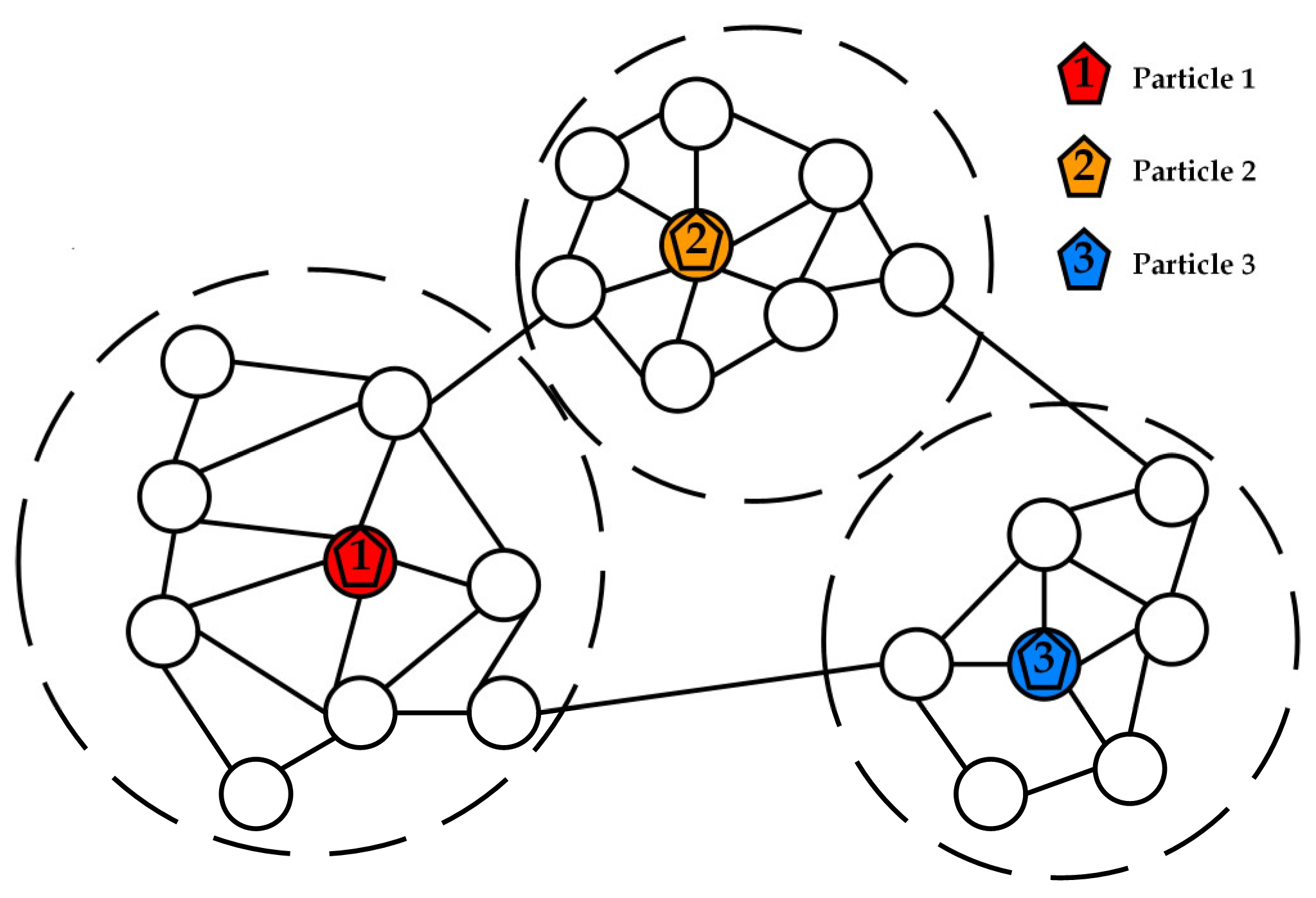
Combining the two aforementioned metrics, the rules for determining particle initialization positions are as follows. Firstly, arrange all nodes in the network in descending order based on their degree values. Select the node with the highest degree value as the starting position for the first particle’s walk. Next, calculate the average Salton similarity index between the node where the already determined starting-position particle is located and all other nodes in the network. Choose the node with the smallest average Salton similarity index as the starting position for the next particle. This process is then repeated iteratively to progressively determine the starting positions for the remaining particles. Finally, when the starting position for each particle is determined, the particle initialization process is completed. Figure 1 depicts the particle initialization position under the condition of three particles. As can be seen from the figure, particles 1, 2, and 3 are dispersed and placed in the network after the position initialization step. $p^{\left(k\right)}\left(0\right)$ denotes the starting position of particle $k$. The rules for determining particle initialization positions can be expressed as follows:

$$p^{\left(k\right)}\left(0\right)=\{\begin{array}{cc}\arg \max \left(d\left(v_i\right)\right),& k=1\\ \arg \min \left(\frac{{\displaystyle \sum _{u=1}^{k-1}Salton\left(j,p^{\left(u\right)}\left(0\right)\right)}}{k}\right),& 2\le k\end{array}$$

(10)

4.2. Incorporating Node Local Similarity into Particle Preferential Movement Rule

The stochastic competitive learning algorithm stipulates that particles navigate through the network based on a convex combination of random walk and preferential walk rules. The preferential walk rule ensures that particles preferentially access nodes under their control, reflecting the deterministic nature of particle traversal, and numerically equivalent to the particle’s control ability ratio. However, this rule solely focuses on the particle’s control ability over nodes, without considering the influence of node local similarity indicators. This may lead to a relatively high degree of randomness and weak inclination in the initial direction of preferential walk, thereby affecting the stability and accuracy of community detection results. To address these issues, an enhancement to the particle preferential walk rule is introduced by incorporating node similarity, enabling nodes with greater similarity to be more likely visited by particles. This modification enhances the directionality and determinism of particle traversal during the walk.

The improved node similarity for the enhanced particle preferential walk rule not only considers cases where nodes share common neighbors, but also accounts for situations where nodes lack common neighbors. When there are shared neighbors between nodes, a similarity index considering both common neighbors and degree difference is employed to measure the degree of similarity between two nodes, as defined below:

$$Sim\left(i,j\right)=\frac{\left|N(v_i)\cap N(v_j)\right|}{\left|N(v_i)\cap N(v_j)\right|+\left|N(v_i)\cup N(v_j)\right|}\times \frac{\left|N(v_i)\cap N(v_j)\right|}{1+\left|N_s-N_h\right|}$$

(11)

For nodes $v_i$ and $v_j$, if $\left|N(v_i)\right|\ge \left|N(v_j)\right|$, then $N_s$ is set to $N(v_j)$, and $N_h$ is set to $N(v_i)$; if $\left|N(v_i)\right|<\left|N(v_j)\right|$, then $N_s$ is set to $N(v_i)$, and $N_h$ is set to $N(v_j)$. When there are no shared neighbors between nodes, further consideration is needed for nodes with a degree value of 1. For nodes without shared neighbors and with a degree value of 1, since their behavior is solely related to their unique first-order neighbor, their similarity value is set to 1. For nodes without shared neighbors and with a degree value greater than 1, their similarity is associated with the node’s degree value. Based on the negative correlation between node degree and the unfavorable Hub Depressed Index, the degree value is inversely related to its similarity. The equation for calculating the similarity between nodes without shared neighbors is defined as follows:

$$Sim\left(i,j\right)=\{\begin{array}{cc}1,& \left(d\left(v_i\right)=1\right)\vee \left(d\left(v_j\right)=1\right)\\ \frac{a_{ij}}{\max \left\{d\left(v_i\right),d\left(v_j\right)\right\}},& d\left(v_i\right)\ne 1,d\left(v_j\right)\ne 1\end{array}$$

(12)

Building upon this, the equation for the particle’s preferential walk rule incorporating node similarity is provided:

$$P_{pref}^{\left(k\right)}\left(i,j,t\right)\triangleq \frac{a_{ij}{\overline{Nu}}_j^{\left(k\right)}\left(t\right)\left(1+Sim\left(i,j\right)\right)}{{\displaystyle \sum _{u\in N(v_i)}{a}_{iu}{\overline{Nu}}_u^{\left(k\right)}\left(t\right)\left(1+Sim\left(i,u\right)\right)}}$$

(13)

where $Sim\left(i,j\right)$ represents the similarity index between nodes $v_i$ and $v_j$, and ${\overline{Nu}}_j^{\left(k\right)}\left(t\right)$ represents the control capacity of particle $k$ over node $v_j$. The improved preferential walk rule takes into account both the particle’s control capacity over nodes and the similarity index between nodes as equally significant factors. This approach avoids the issue of randomness in the preferential walk direction that arises after particle initialization, thereby enhancing the inclination and certainty of particle movement throughout the entire preferential walk process.

4.3. Dynamically Adjusting Particle Control Capacity Increment

In the Stochastic Competitive Learning algorithm, the control capacity of particles is quantified as the proportion of node visits, thereby the number of times a particle visits a node determines its control capacity over that node. When particle $k$ visits node $v_i$, the equation for the change in the particle’s visit count to that node is given by:

$$N{u}_i^{\left(k\right)}\left(t+1\right)=N{u}_i^{\left(k\right)}\left(t\right)+1$$

(14)

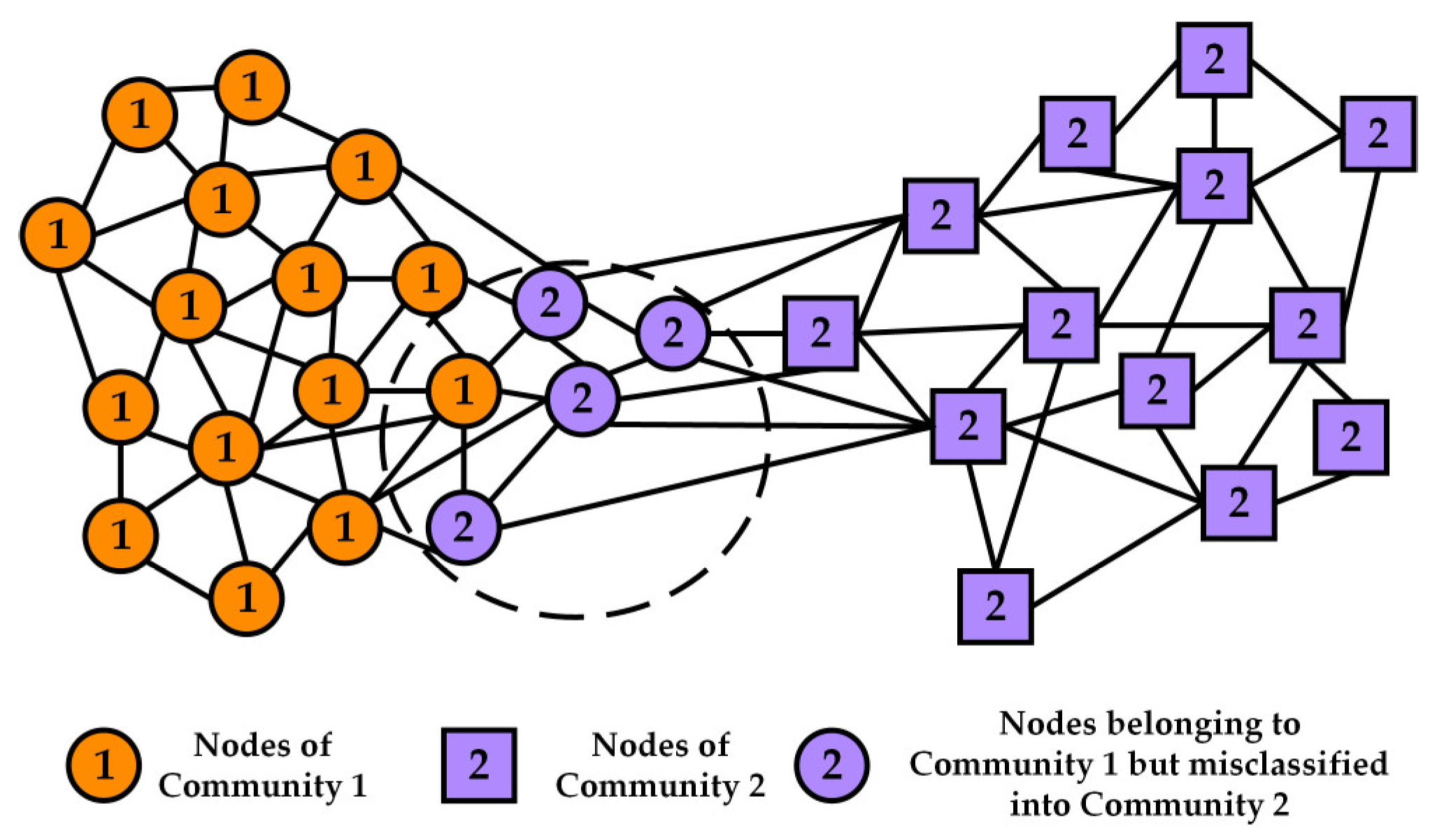
According to Equation (14), it can be observed that the increment of particle control capacity remains constant at 1. This would lead to particles having the same level of competitive increment during the walking process. This uniform competitive increment among different particles could potentially result in similar community sizes controlled by different particles. Consequently, this might lead to instances where representative particles of smaller communities erroneously compete for nodes at the boundaries of larger communities. However, many real-life complex systems, represented as complex networks, often encompass communities of varying sizes. The constant increment in particle control capacity could potentially yield suboptimal results in the final community detection outcome. Figure 2 depicts the possible encroachment of a small community into a large community node when the particle control capacity increment is constant. The size of community 1 in the figure is actually larger than that of community 2. However, because of the constant particle control capacity increment, it makes it possible for the range of communities controlled by each particle to converge to the same size. This then causes nodes that should belong to community 2 to be misclassified to community 2.

Addressing the aforementioned issues, an improvement is made to the particle control capacity increment in order to enhance the effectiveness of discovering communities of varying sizes within the network. The enhanced particle control capacity increment is dynamically adjusted based on the current control range of the particle, and the specific equation is provided below:

$$N{u}_i^{\left(k\right)}\left(t+1\right)=N{u}_i^{\left(k\right)}\left(t\right)+1+\frac{\left|C^{\left(k\right)}\left(t\right)\right|}{\left|V\right|}$$

(15)

where $\left|C^{\left(k\right)}\left(t\right)\right|$ represents the current control range of particle $k$, which indicates the number of nodes currently under the control of particle $k$. From Equation (15), it can be observed that the particle’s control capacity increment is positively correlated with its current control range. This relationship can unveil community structures of different sizes within the network and prevent particles from erroneously encroaching upon nodes located at the boundaries of communities.

4.4. Determining Particle Resurrection Locations and Node Affiliation Selection

In stochastic competitive learning, when a particle visits a node under its control, its energy increases. On the other hand, when it visits a node controlled by a competing particle, its energy decreases. This energy manipulation serves to constrain the particle’s walking range, thus reducing long-range and redundant accesses in the network. If a particle frequently visits nodes controlled by competing particles, its energy will continuously decrease until it is exhausted and enters a dormant state. Subsequently, the particle will randomly jump to a node within its control range to revive and recharge.

Clearly, the choice of the particle’s revival location has a high degree of randomness, which can lead to unstable community detection results. To address this issue, based on the particle’s control over nodes, we select the node with the highest control capability as the unique revival location among the nodes it already controls, eliminating the uncertainty in location selection. If a particle currently doesn’t control any nodes, it will randomly choose any node in the network for revival. The improved particle revival location selection is shown in Figure 3, where the energy of particle 1 is depleted due to its traversal into the control region of particle 3. After the improvement, particle 1 will no longer randomly jump to any controlled node within the dashed box, but will instead jump to the node indicated by the dashed arrow (assuming that node has the highest control capability value for particle 1).

Once the algorithm reaches the convergence criterion, particles will cease their walks. Based on the control capabilities of each particle over nodes, all nodes in the network are assigned to the corresponding communities represented by particles. However, due to the potential randomness and potential misclassifications in the steps executed by particles before stopping their walks, a node membership selection step is introduced. By considering the frequency of community labels among neighboring nodes, this step ensures that each node is correctly assigned to its appropriate community, further optimizing the community detection outcomes. Specifically, for each node, the occurrence frequency of community labels among its neighboring nodes is observed. If the most frequent neighboring community label is unique, it is selected as the community label for that node. If the most frequent neighboring community label is not unique, an influence score is computed for each community, and the community label with the highest influence score is selected. The influence score $Effec{t}_{C_k}$ for a community is calculated as shown in the equation below:

$$Effec{t}_{C_k}={\displaystyle \sum _{j\in N\left(v_i\right)}Sim\left(i,j\right)},j\in C_k$$

(16)

where $C_k$ is one of the most frequent communities, and $N\left(v_i\right)$ represents the set of neighboring nodes of node $v_i$.

4.5. Algorithm Description

Algorithm 1 describes the method of the LNSSCL algorithm; the pseudocode is shown below.

Algorithm 1 LNSSCL algorithm

Input: Graph $G=(V,E)$             The probability of preferential walk for particles $\lambda$,

Particle energy increment $\Delta$, Convergence factor $\epsilon$

Output: The number of communities $K$, The set of communities $C$

1:         $t=1$

2:         $K=2$

3:         repeat

1:                 for each particle $k$ do:

5:                         calculate the initial positions of particles $p^{\left(k\right)}\left(0\right)$ using Equation (10)

6:                 end for

7:                 repeat

8:                        for $k=1$ to $K$ do:

9:                                 calculate the particle’s random walk probability $P_{rand}^{\left(k\right)}\left(i,j\right)$ using Equation (4)

10:                                 calculate the particle’s preferential walk probability $P_{pref}^{\left(k\right)}\left(i,j,t\right)$ using Equation (11), (12), and (13)

11:                                 calculate the particle’s walk probability $P_{transition}^{\left(k\right)}\left(i,j,t\right)$ using Equation (3)

12:                                 particles walk based on the walk probability and dynamically adjust the particle’s control increment using Equation (15)

13:                                if $E^{\left(k\right)}\left(0\right)\le 0$:

14:                                         particle performs the revival step by jumping to the node within their control range that possesses the maximum control capability for revival and re-energization.

15:                                 end if

16:                         end for

17:                         update $Nu\left(t\right)$, $\overline{Nu\left(t\right)}$, $E\left(t\right)$, $S\left(t\right)$

18:                         $t=t+1$

19:                until Equation (7) is satisfied

20:                 calculating and record the average maximum control capability indicator for particles $\langle R\left(t\right)\rangle$ using Equation (8).

21:                 $K=K+1$

22:        until $\langle R\left(t\right)\rangle$ reaches its maximum value

23:        assign the number of particles corresponding to step 22 to $K$

24:        for each node $v_i\in V$do:

25:                 Assign the corresponding community label to node $v_i$ based on the mag- nitude relationship of ${\overline{Nu}}_i\left(t\right)$

26:         end for

27:        for each node $v_i\in V$do:

28:                 get the set of neighboring nodes $N(v_i)$ for node $v_i$ and count the frequen- cy of appearance of community labels for each neighboring node

29:                if the most frequently occurring neighboring community label is unique:

30:                         the label of node $v_i$ is updated to the most frequently occurring community label.

31:                else:

32:                         calculate the power score of each most frequent community $Effec{t}_{C_k}$ using Equation (16)

33:                         the label of node $v_i$ is updated to the community label with the highest community effectiveness score

34:                 end if

35:         end for

36:        return $K-1$, $C$

4.6. Time Complexity Analysis

For a complex network $G=(V,E)$, assuming the average degree of nodes is $\overline{d}$, the number of nodes is $n$, the number of edges is $m$, and the common neighbors between two nodes is $c$. The determination of particle starting positions involves calculating node degrees and the Salton similarity index between nodes, with a time complexity of $O\left(m\right)$. Active particles wandering in the network require calculating the probability for each particle to move from the current node to neighboring nodes. The random walk probability for each particle only requires computing node degrees, while the preferential walk probability needs to calculate the similarity index between the current node and its neighbors, with a time complexity of $O\left(Kc\overline{d}\right)$. When a particle’s energy is exhausted, the revival step involves maintaining a hash table to store each particle’s control nodes and their corresponding control capability values. Finding the node with the maximum control capability for jumping has a time complexity of $O\left(1\right)$. Updating the particle control matrix has a time complexity of $O\left(K^2\right)$. Since each node in the network is visited at least once by a particle, the total time complexity of particle wandering is $O\left(Kc\overline{d}n+K^{2}n\right)$. To determine the optimal number of particles, the algorithm needs to gradually change the particle count from 2 to $K^{\prime }$, where $K^{\prime }$ is a constant slightly larger than the actual number of communities in the network. Therefore, the entire particle wandering process of the LNSSCL algorithm has a time complexity of $O\left(K^{2}c\overline{d}n+K^{3}n\right)$. After the particle wandering process concludes, assigning community labels to all nodes based on their control capability values requires a time complexity of $O\left(n\right)$. The node membership selection step involves each node selecting its community label based on the frequency of community labels among its neighboring nodes, with a time complexity of $O\left(\left(\overline{d}+c{\overline{d}}^2\right)n\right)$. Since complex networks are usually sparse networks, $\overline{d}\ll n$. In summary, the time complexity of the LNSSCL algorithm is $O\left(m+K^{2}c\overline{d}n+K^{3}n+\left(\overline{d}+c{\overline{d}}^2\right)n\right)\approx O\left(M\left(m+n\right)\right)$, where $M$ is a constant. The time complexity of the LNSSCL algorithm is linearly related to the sum of the number of nodes and edges in the network, making the algorithm highly scalable on large-scale networks.

5. Experiments and Discussions

To test the effectiveness of the LNSSCL algorithm, experiments were conducted on real network datasets and synthetic networks, comparing the proposed algorithm with 12 representative community detection algorithms. The selected benchmark algorithms for experimentation include community detection algorithms based on random walk such as Walktrap [23] and Infomap [24]; modularity-based algorithms CNM [36], Louvain [37], and Leiden [38]; label propagation-based algorithms LPA [39], TS [27], GLLPA [29], and SSCLPA [30]; hierarchical clustering algorithm Paris [40], Markov chain-based community detection algorithm MSC [25], and the stochastic competitive learning algorithm based on the particle competition mechanism SCL [14].

5.1. Experimental Environment and Initial Parameters

The algorithm was implemented using NetworkX and scikit-learn. The specific experimental environment is shown in

Table 1. Experimental environment parameters.

Hardware/Software	Configuration
OS	Windows 11 Home
CPU	Intel(R) Core(TM) i5-11400H @ 2.70GHz
RAM	16 GB
GPU	NVIDIA GeForce RTX 3050 Ti Laptop
Anaconda	3.9.12
Python	3.7.12
NetworkX	2.6.3
scikit-learn	1.0.2

.

For the setting of the initial parameters, we refer to the value range of the literature [35]. The value range of the particle preferential wandering probability parameter $\lambda$ is $\left[0.2,0.8\right]$, and we set its initial value to 0.6; the value range of the particle energy update value $\Delta$ is $\left[0.1,0.4\right]$, and we set its initial value to 0.3; the convergence factor $\epsilon$ is set to 0.05; and the minimum value of the particle energy $E_{\min }$ is set to 0, and the maximum value of the particle energy $E_{\max }$ is set to 1.

5.2. Datasets

The experiment utilized 11 real network datasets, including four labeled real network datasets and seven unlabeled real network datasets. The labeled real network datasets consist of the Karate network [41], Dolphins network [42], Polbooks network [43], and Football network [1]. The unlabeled real network datasets include the Lesmis network [44], Jazz network [45], Email network [46], Netscience network [47], Power Grid network [48], Facebook network [49], and PGP network [50]. The basic information is presented in

Table 2. Basic information of real network datasets.

Dataset	Nodes	Edges	Community
Karate	34	78	2
Dolphins	62	159	2
Polbooks	105	441	3
Football	115	613	12
Lesmis	77	254	-
Jazz	198	5484	-
Email	1133	5451	-
Netscience	1589	2742	-
Power Grid	4941	6594	-
Facebook	4039	88,234	-
PGP	10,680	24,316	-

.

Likewise, to expand experiments, the LFR benchmark is used as synthetic networks [51]. We generate different scale networks on the LFR test network model for experiments. The specific parameter settings of the LFR network are shown in

Table 3. The parameters for LFR network construction.

Network	$\mathit{n}$	$\overline{\mathit{d}}$	${\mathit{d}}_{\mathbf{max}}$	$\mathbf{min}\mathit{c}$	$\mathbf{max}\mathit{c}$	$\mathit{t}\mathit{a}\mathit{u}1$	$\mathit{t}\mathit{a}\mathit{u}2$	$\mathit{\mu }$
LFR1	1000	15	50	20	100	2	1.1	0.1–0.8
LFR2	4000	15	50	20	100	2	1.1	0.1–0.8

, where $\overline{d}$ is average degree, $d_{\max }$ denotes maximum degree, $\min c$ represents minimum community size, $\max c$ is maximum community size, and $tau1$ and $tau2$ are the parameters for power law distribution. $\mu$ is the mixed parameter. The larger the mixed parameter, the more difficult the community division.

5.3. Evaluation Index

In this paper, we use two widely adopted evaluation metrics for community detection algorithms to assess the quality of the algorithm’s community detection results. For labeled real network datasets, we utilize Normalized Mutual Information (NMI) [52] and modularity [36] to evaluate the community detection results of each algorithm. For unlabeled real-world network datasets, since the ground-truth community structures of these network datasets are still unknown, we assess the quality of the detected results in terms of the modularity only. For LFR networks, we use NMI to evaluate the community detection results of each algorithm.

The NMI score is defined as shown in Equation (17):

$$NMI(X,Y)=\frac{-2{\displaystyle \sum _{i=1}^{C_X}{\displaystyle \sum _{j=1}^{C_Y}{C}_{ij}\mathrm{lb}\left(\frac{C_{ij}N}{C_i{C}_j}\right)}}}{{\displaystyle \sum _{i=1}^{C_X}{C}_i\mathrm{lb}\left(\frac{C_i}{N}\right)+{\displaystyle \sum _{j=1}^{C_Y}{C}_j\mathrm{lb}\left(\frac{C_j}{N}\right)}}}$$

(17)

where $X$ represents the ground truth community structure and $Y$ represents the community detection results of the algorithm. $C_X$ denotes the number of true communities in the ground truth, and $C_Y$ represents the number of communities detected by the algorithm. $C$ represents the confusion matrix, where rows represent the ground truth community structure and columns represent the algorithm’s community detection results. $C_{ij}$ represents the number of common nodes between the true community $i$ in $X$ and the community $j$ detected in $Y$. $C_i$ represents the sum of row $i$ in matrix $C$, and $C_j$ represents the sum of row $j$ in matrix $C$. $N$ stands for the total number of nodes in the network. $NMI\in [0,1]$. A higher NMI value indicates a better agreement between the algorithm’s community detection results and the true community structure, thus implying a better performance of community detection.

The modularity(Q) is defined as shown in Equation (18):

$$Q=\frac{1}{2m}{\displaystyle \sum _{i,j}\left(a_{ij}-\frac{d\left(v_i\right)\times d\left(v_j\right)}{2m}\right)}\times \delta \left(c_i,c_j\right)$$

(18)

where $m$ denotes the number of edges in the network, $a_{ij}$ denotes the connection status between node $v_i$ and node $v_j$; $c_i$ denotes the community label of node $v_i$, $c_j$ denotes the community label of node $v_j$; $\delta \left(c_i,c_j\right)$ denotes the Kronecker function, which takes the value 1 if $c_j$ and $c_j$ are the same; otherwise, it takes the value 0. Generally, a larger modularity value implies a more distinct community structure.

5.4. Experimental Results and Analysis

5.4.1. Experimental Results and Analysis on Labeled Real Network Datasets

On the four labeled real network datasets, namely Karate, Dolphins, Polbooks, and Football, we conducted comparative experiments between the proposed LNSSCL algorithm and 12 other representative community detection algorithms. We evaluated the community detection results of each algorithm using NMI score and modularity Q. The experimental results are shown in

Table 4. Comparison of the NMI of each algorithm on labeled real network datasets. The largest NMI are in bold.

Algorithm	Karate	Dolphins	Polbooks	Football
Walktrap	0.504	0.582	0.543	0.887
Infomap	0.699	0.417	0.529	0.911
CNM	0.692	0.557	0.531	0.698
Louvain	0.587	0.484	0.569	0.885
Leiden	0.687	0.581	0.574	0.890
LPA	0.445	0.595	0.534	0.870
TS	0.710	0.888	0.550	0.900
GLLPA	0.753	0.790	0.580	0.909
SSCLPA	0.826	0.616	0.493	0.919
Paris	0.835	0.780	0.565	0.831
MSC	0.836	0.777	0.539	0.921
SCL	0.821	0.816	0.552	0.861
LNSSCL	0.848	0.899	0.610	0.937

and

Table 5. Comparison of modularity Q of each algorithm on labeled real network datasets. The largest Q are in bold.

Algorithm	Karate	Dolphins	Polbooks	Football
Walktrap	0.353	0.489	0.507	0.603
Infomap	0.401	0.532	0.521	0.600
CNM	0.381	0.495	0.502	0.550
Louvain	0.415	0.516	0.526	0.602
Leiden	0.420	0.527	0.527	0.602
LPA	0.375	0.499	0.481	0.583
TS	0.420	0.381	0.520	0.600
GLLPA	0.438	0.496	0.507	0.608
SSCLPA	0.415	0.525	0.518	0.601
Paris	0.372	0.380	0.426	0.510
MSC	0.418	0.495	0.519	0.600
SCL	0.371	0.463	0.508	0.581
LNSSCL	0.424	0.532	0.524	0.613

.

As can be seen in Table 4 and Table 5, the LNSSCL algorithm achieves the highest NMI values on all labeled real network datasets and has some degree of improvement over the other algorithms. Whereas, for the comparison of modularity Q, the LNSSCL algorithm does not take the optimal value on all the datasets. Though the proposed algorithm took the highest value only on Dolphins and Football datasets, the modularity scores on Karate and Polbooks datasets were close to the highest level.

The NMI measures the similarity between the algorithm’s output community segmentation results and the real online community structure. The larger the NMI, the higher the similarity between the algorithm’s output community segmentation results and the real online community structure. It can be seen that the community detection results of the LNSSCL algorithm on the four labeled real network datasets of Karate, Dolphins, Polbooks, and Football are closest to the real community structure of the above networks. In addition, the LNSSCL algorithm improves its NMI values by 3.3%, 10.2%, 10.5%, and 8.8% on the Karate, Dolphins, Polbooks, and Football datasets, respectively, compared to the SCL algorithm. This demonstrates the effectiveness of a series of improvements to the SCL algorithm by the LNSSCL algorithm, which improves the stability and accuracy of the SCL algorithm.

For other algorithms, CNM, Louvain, and Leiden algorithms seek to maximize the modularity of the whole network, which obtains good modularity scores but fails to discover the real community structure well. LPA, TS, GLLPA, and SSCLPA algorithms tend to have a certain degree of randomness in the node order of label updating and the label propagation process, making the final community. The computational complexity of Walktrap and Infomap, two randomized wandering algorithms, is relatively high and sensitive to the parameters set by themselves. Due to the small size of the dataset used in the experiments and the existence of small communities, although they have higher modularity scores, they failed to achieve higher NMI scores, and the consistency with the real community structure is insufficient.

Overall, the LNSSCL algorithm works best for community detection on the Karate, Dolphins, Polbooks, and Football datasets.

5.4.2. Experimental Results and Analysis on Unlabeled Real Network Datasets

On the seven unlabeled real network datasets, namely Lesmis, Jazz, Email, Netscience, Power Grid, Facebook, and PGP, the proposed LNSSCL algorithm was compared against 12 representative learning algorithms through experimental evaluation. The assessment of various algorithm’s community detection outcomes was conducted using modularity Q, and the experimental results are shown in

Table 6. Comparison of modularity Q of each algorithm on unlabeled real network datasets. The largest Q are in bold.

Algorithm	Lesmis	Jazz	Email	Netscience	Power Grid	Facebook	PGP
Walktrap	0.521	0.438	0.531	0.956	0.831	0.812	0.832
Infomap	0.546	0.442	0.538	0.930	0.759	0.706	0.821
CNM	0.501	0.439	0.503	0.955	0.935	0.777	0.853
Louvain	0.527	0.282	0.463	0.907	0.627	0.835	0.885
Leiden	0.558	0.443	0.563	0.959	0.935	0.836	0.887
LPA	0.560	0.445	0.574	0.960	0.939	0.737	0.745
TS	0.535	0.440	0.550	0.924	0.930	0.796	0.767
GLLPA	0.556	0.440	0.292	0.920	0.784	0.785	0.786
SSCLPA	0.557	0.406	0.513	0.906	0.838	0.779	0.801
Paris	0.504	0.276	0.451	0.876	0.405	0.586	0.679
MSC	0.544	0.447	0.565	0.948	0.890	0.812	0.872
SCL	0.539	0.411	0.550	0.932	0.863	0.804	0.815
LNSSCL	0.575	0.463	0.585	0.971	0.952	0.847	0.896

.

Since the unlabeled network dataset is without real community structure, we can accomplish community delineation by identifying structural features with strong internal connections and sparse external connections. Modularity measures the strength of community structure in the network and evaluates the results of algorithmic community delineation when the dataset has no real community structure. The larger the modularity degree is, the better the quality of community detection and the stronger the connection within the community.

As can be seen in Table 6, the LNSSCL algorithm achieves the maximum modularity on all seven unlabeled network datasets used in the experiments, outperforming other comparison algorithms. In addition, these network datasets are of different types, sizes, and sparsities, and the high modularity performance of the LNSCCL algorithm reflects the algorithm’s good generalization and universality. In particular, the performance on two larger datasets, Facebook and PGP, shows that the algorithm has some scalability. For other algorithms, CNM, Louvain, and other algorithms oriented to maximize the modularity achieved high modularity on the Netscience, Power Grid, Facebook, and PGP datasets, with Leiden in particular being the most prominent, but did not show the best performance on the smaller datasets. LPA, TS, GLLPA, and SSCLPA algorithms are not as effective as the stable LNSSCL algorithm in the experiments, because some randomness in the node order of the label update and label propagation process cannot show stable and accurate performance. The MSC algorithm constructs a steady-state Markov similarity augmented matrix, which is capable of stable and efficient community delineation, and achieves high modularity in the experiments. Further, the NSSCL algorithm improves its modularity values by 6.7%, 12.7%, 6.4%, 4.2%, 10.3%, 5.3%, and 9.9% on Lesmis, Jazz, Email, Netscience, Power Grid, Facebook, and PGP datasets, respectively, as compared to the SCL algorithm. This shows that the LNSSCL algorithm improves the stability and accuracy of the original SCL algorithm for community detection to some extent.

5.4.3. Experimental Results and Analysis on synthetic networks

In order to better measure the performance of the algorithm, we generate networks of different sizes for experiments on the LFR test network model. In this case, the number of nodes in the LFR1 network is 1000 and the number of nodes in the LFR2 network is 4000. Since the real community structure of the LFR network is known, the performance of the algorithm is measured using NMI. Among the important parameters used to create the LFR network, the mixing parameter $\mu$ is used to represent the complexity of the community structure and determines the clarity of the community structure. As the mixing parameter $\mu$ increases, the community structure becomes more complex and the difficulty of recognizing the community increases. The experimental results of the LFR network with different mixing parameter $\mu$ are shown in Figure 4, where the horizontal coordinates represent the individual values of the mixing parameter μ and the vertical coordinates represent the NMI.

As can be seen in Figure 4, the performance of each algorithm decreases to varying degrees in both sets of networks as the mixing parameter μ increases, but the community detection performance of the LNSSCL algorithm still outperforms most of the compared algorithms.

When the mixing parameter μ is less than 0.4, the algorithms have higher NMI values, except for the CNM and Paris algorithms. When μ is greater than 0.4, the NMIs all show a decrease. Among them, label propagation-based algorithms such as LPA have very obvious changes in decline, especially the LPA algorithm, which has an NMI value of 0 in both networks when μ is not less than 0.6. The reason for the analysis is that label propagation-based algorithms have a certain degree of randomness, which is prone to cause low performance and instability in community detection when the community structure is not clear enough. Comparing the synthetic networks LFR1 and LFR2, the NMI of most of the algorithms increased with the increase in the number of nodes. However, the performance of the CNM algorithm shows a decrease, which is attributed to the fact that the algorithm may have the problem of resolution limitation when dealing with networks with larger communities, and is unable to decompose large communities into smaller sub-communities. From Figure 4, it can be found that the NMI value of LNSSCL tends to 1 when μ = 0.1, and the NMI value of LNSSCL is maximum when μ = 0.8. It indicates that the performance of LNSSCL decays the slowest, i.e., the performance of LNSSCL is more stable.

In summary, the community detection results of the LNSSCL algorithm are better on synthetic network datasets generated with different parameters.

5.4.4. Parameter Sensitivity Analysis

In this section, we focus on the effects of the parameters $\lambda$ and $\Delta$ on the LNSSCL algorithm. $\lambda$ represents the probability of a particle performing preferential walk, regulating the balance between random and preferential walking. When the parameter $\lambda$ takes a relatively low value, the particles are more inclined to wander randomly, visit new nodes, and expand the community range, but are prone to the problem of too much randomness. When the parameter $\lambda$ takes a relatively high value, the particle is more inclined to preferentially wander, frequently visit the nodes that have been controlled, and consolidate the community scope, but it is easy to fall into the localized area and it cannot visit new nodes. From Figure 5, it can be seen that the parameter $\lambda$ can achieve the best community detection performance by appropriately increasing the value of the parameter when balancing random wandering and preferential wandering ($\lambda =0.5$). For the Polbooks, Football, and Jazz datasets, the best performance is achieved when the value of $\lambda$ is 0.6, while the Email dataset takes the value of λ as 0.5.

The parameter $\Delta$ is responsible for updating the particle’s energy value. When $\Delta$ is very small, the particle is not penalized enough by the energy it receives for visiting nodes that are not under its control, so the particle’s energy will not be depleted during its wanderings. The particle will frequently visit nodes that should belong to the nodes to which the competing particles belong and enter the core of other communities. As a result, all nodes in the network will be in constant competition, unable to establish and consolidate community boundaries, and the final community detection will be less effective. When $\Delta$ is very large, the particle will simply run out of energy once it visits a node controlled by a competing particle. The particle will frequently enter the resurrection phase and is not expected to move away from its initial position to take control of other nodes. As can be seen in Figure 6, a parameter $\Delta$ of 0.3 achieves the best performance on all four datasets of the experiment. The different values of the parameter $\Delta$ have roughly the same trend in affecting the performance on different datasets in the experiment.

According to Figure 5 and Figure 6, the algorithm is somewhat sensitive to the values of $\lambda$ and $\Delta$. Numerically, there is little fluctuation within a small interval of relative range. Based on the results of the parameter sensitivity analysis experiments, we set $\lambda$ to 0.6 and $\Delta$ to 0.3 for experiments on other datasets.

6. Conclusions and Future Work

This paper introduces a novel unsupervised community detection algorithm named LNSSCL, which incorporates node local similarity into the process of stochastic competitive learning. Firstly, the algorithm determines the starting position of particles’ walks by calculating the degree value of nodes as well as the Salton similarity index. At the same time, the fusion of node similarity optimizes the particle preferential walk rule. During the particle wandering process, the particle control capacity increment is dynamically adjusted according to the control range of each particle. When a particle runs out of energy, the particle selects the node with the largest control power within its control range for resurrection. After the particle stops wandering, the nodes in the network are selected for affiliation based on the frequency of occurrence of community labels of neighboring nodes and the effectiveness score of neighboring communities, and the community detection results are finally obtained. Comparative experiments on real network datasets and synthetic networks show that the LNSSCL algorithm is effective in improving the SCL algorithm. Compared with other representative algorithms, the LNSSCL algorithm has better quality of community detection and is able to reveal a more reasonable community structure.

Nevertheless, the LNSSCL algorithm also has some defects. Compared with the SCL algorithm, the algorithm performs multiple node local similarity calculations during the community detection process, which requires more computational cost and complexity, and may have a larger time overhead on ultra-large networks. In the selection of some hyperparameters of the algorithm, no special parameter tuning method is used; the parameters are tuned manually. Further, the networks studied in this paper are simple undirected networks and not complex networks that are closer to the real world, such as directed, weighted, or attribute. In the next step of this study, we can consider optimizing the similarity calculation to further reduce the time overhead, adopting a dynamic adaptive hyper-parameter tuning strategy instead of traditional parameter tuning. GNN is introduced to fuse attribute information and structural features to obtain node representations and calculate node representation similarity to study the community detection strategy for attribute networks.

References

1. Girvan, M.; Newman, M.E. Community Structure in Social and Biological Networks. Proc. Natl. Acad. Sci. USA 2002, 99, 7821–7826. [Google Scholar] [CrossRef]
2. Fortunato, S. Community Detection in Graphs. Phys. Rep. 2010, 486, 75–174. [Google Scholar] [CrossRef]
3. Fortunato, S.; Hric, D. Community Detection in Networks: A User Guide. Phys. Rep. 2016, 659, 1–44. [Google Scholar] [CrossRef]
4. Javed, M.A.; Younis, M.S.; Latif, S.; Qadir, J.; Baig, A. Community Detection in Networks: A Multidisciplinary Review. J. Netw. Comput. Appl. 2018, 108, 87–111. [Google Scholar] [CrossRef]
5. Jin, D.; Yu, Z.; Jiao, P.; Pan, S.; He, D.; Wu, J.; Yu, P.; Zhang, W. A Survey of Community Detection Approaches: From Statistical Modeling to Deep Learning. IEEE Trans. Knowl. Data Eng. 2021, 35, 1149–1170. [Google Scholar] [CrossRef]
6. Xing, S.; Shan, X.; Fanzhen, L.; Jia, W.; Jian, Y.; Chuan, Z.; Wenbin, H.; Cecile, P.; Surya, N.; Di, J. A Comprehensive Survey on Community Detection with Deep Learning. IEEE Trans. Neural Netw. Learn. Syst 2022, 1–21. [Google Scholar] [CrossRef]
7. Wang, B.; Gu, Y.; Zheng, D. Community Detection in Error-Prone Environments Based on Particle Cooperation and Competition with Distance Dynamics. Phys. A Stat. Mech. Its Appl. 2022, 607, 128178. [Google Scholar] [CrossRef]
8. Grossberg, S. Competitive Learning: From Interactive Activation to Adaptive Resonance. Cogn. Sci. 1987, 11, 23–63. [Google Scholar] [CrossRef]
9. Kohonen, T. The Self-Organizing Map. Proc. IEEE 1990, 78, 1464–1480. [Google Scholar] [CrossRef]
10. Kohonen, T.; Kohonen, T. Learning Vector Quantization. Self-Organ. Maps 1995, 30, 175–189. [Google Scholar]
11. Hecht-Nielsen, R. Counterpropagation Networks. Appl. Opt. 1987, 26, 4979–4984. [Google Scholar] [CrossRef] [PubMed]
12. Kosko, B. Stochastic Competitive Learning. In Proceedings of the 1990 IJCNN International Joint Conference on Neural Networks, San Diego, CA, USA, 17–21 June 1990; IEEE: New York, NY, USA, 1990; pp. 215–226. [Google Scholar]
13. Quiles, M.G.; Zhao, L.; Alonso, R.L.; Romero, R.A. Particle Competition for Complex Network Community Detection. Chaos Interdiscip. J. Nonlinear Sci. 2008, 18, 033107. [Google Scholar] [CrossRef] [PubMed]
14. Silva, T.C.; Zhao, L. Stochastic Competitive Learning in Complex Networks. IEEE Trans. Neural Netw. Learn. Syst. 2012, 23, 385–398. [Google Scholar] [CrossRef] [PubMed]
15. Silva, T.C.; Zhao, L. Detecting and Preventing Error Propagation via Competitive Learning. Neural Netw. 2013, 41, 70–84. [Google Scholar] [CrossRef] [PubMed]
16. Silva, T.C.; Zhao, L. Uncovering Overlapping Cluster Structures via Stochastic Competitive Learning. Inf. Sci. 2013, 247, 40–61. [Google Scholar] [CrossRef]
17. Li, W.; Gu, Y.; Yin, D.; Xia, T.; Wang, J. Research on the Community Number Evolution Model of Public Opinion Based on Stochastic Competitive Learning. IEEE Access 2020, 8, 46267–46277. [Google Scholar] [CrossRef]
18. Zamoner, F.W.; Zhao, L. A Network-Based Semi-Supervised Outlier Detection Technique Using Particle Competition and Cooperation. In Proceedings of the 2013 Brazilian Conference on Intelligent Systems, Fortaleza, Brazil, 19–24 October 2013; IEEE: New York, NY, USA, 2013; pp. 225–230. [Google Scholar]
19. Breve, F.; Quiles, M.G.; Zhao, L. Interactive Image Segmentation Using Particle Competition and Cooperation. In Proceedings of the 2015 international joint conference on neural networks (IJCNN), Killarney, Ireland, 12–17 July 2015; IEEE: New York, NY, USA, 2015; pp. 1–8. [Google Scholar]
20. Breve, F.; Fischer, C.N. Visually Impaired Aid Using Convolutional Neural Networks, Transfer Learning, and Particle Competition and Cooperation. In Proceedings of the 2020 International Joint Conference on Neural Networks (IJCNN), Glasgow, UK, 19–24 July 2020; IEEE: New York, NY, USA, 2020; pp. 1–8. [Google Scholar]
21. Roghani, H.; Bouyer, A. A Fast Local Balanced Label Diffusion Algorithm for Community Detection in Social Networks. IEEE Trans. Knowl. Data Eng. 2022, 35, 5472–5484. [Google Scholar] [CrossRef]
22. Toth, C.; Helic, D.; Geiger, B.C. Synwalk: Community Detection via Random Walk Modelling. Data Min. Knowl. Discov. 2022, 36, 739–780. [Google Scholar] [CrossRef]
23. Pons, P.; Latapy, M. Computing Communities in Large Networks Using Random Walks. In Proceedings of the Computer and Information Sciences-ISCIS 2005: 20th International Symposium, Istanbul, Turkey, 26–28 October 2005; Proceedings 20. Springer: Berlin/Heidelberg, Germany, 2005; pp. 284–293. [Google Scholar]
24. Rosvall, M.; Bergstrom, C.T. Maps of Random Walks on Complex Networks Reveal Community Structure. Proc. Natl. Acad. Sci. USA 2008, 105, 1118–1123. [Google Scholar] [CrossRef]
25. Yang, X.-H.; Ma, G.-F.; Zeng, X.-Y.; Pang, Y.; Zhou, Y.; Zhang, Y.-D.; Ye, L. Community Detection Based on Markov Similarity Enhancement. IEEE Trans. Circuits Syst. II Express Briefs 2023, 70, 3664–3668. [Google Scholar] [CrossRef]
26. Jokar, E.; Mosleh, M.; Kheyrandish, M. Discovering Community Structure in Social Networks Based on the Synergy of Label Propagation and Simulated Annealing. Multimed. Tools Appl. 2022, 81, 21449–21470. [Google Scholar] [CrossRef]
27. You, X.; Ma, Y.; Liu, Z. A Three-Stage Algorithm on Community Detection in Social Networks. Knowl.-Based Syst. 2020, 187, 104822. [Google Scholar] [CrossRef]
28. Dabaghi-Zarandi, F.; KamaliPour, P. Community Detection in Complex Network Based on an Improved Random Algorithm Using Local and Global Network Information. J. Netw. Comput. Appl. 2022, 206, 103492. [Google Scholar] [CrossRef]
29. Zhang, Y.; Liu, Y.; Jin, R.; Tao, J.; Chen, L.; Wu, X. Gllpa: A Graph Layout Based Label Propagation Algorithm for Community Detection. Knowl.-Based Syst. 2020, 206, 106363. [Google Scholar] [CrossRef]
30. Chin, J.H.; Ratnavelu, K. Community Detection Using Constrained Label Propagation Algorithm with Nodes Exemption. Computing 2022, 104, 339–358. [Google Scholar] [CrossRef]
31. Fei, R.; Wan, Y.; Hu, B.; Li, A.; Li, Q. A Novel Network Core Structure Extraction Algorithm Utilized Variational Autoencoder for Community Detection. Expert Syst. Appl. 2023, 222, 119775. [Google Scholar] [CrossRef]
32. Li, H.-J.; Wang, L.; Zhang, Y.; Perc, M. Optimization of Identifiability for Efficient Community Detection. New J. Phys. 2020, 22, 063035. [Google Scholar] [CrossRef]
33. Lü, L.; Zhou, T. Link Prediction in Complex Networks: A Survey. Phys. A Stat. Mech. Its Appl. 2011, 390, 1150–1170. [Google Scholar] [CrossRef]
34. Silva, T.C.; Amancio, D.R. Network-Based Stochastic Competitive Learning Approach to Disambiguation in Collaborative Networks. Chaos: Interdiscip. J. Nonlinear Sci. 2013, 23, 013139. [Google Scholar] [CrossRef]
35. Silva, T.C.; Zhao, L. Case Study of Network-Based Unsupervised Learning: Stochastic Competitive Learning in Networks. In Machine Learning in Complex Networks; Springer International Publishing: Cham, Switzerland, 2016; pp. 241–290. ISBN 978-3-319-17289-7. [Google Scholar]
36. Clauset, A.; Newman, M.E.; Moore, C. Finding Community Structure in Very Large Networks. Phys. Rev. E 2004, 70, 066111. [Google Scholar] [CrossRef]
37. Blondel, V.D.; Guillaume, J.-L.; Lambiotte, R.; Lefebvre, E. Fast Unfolding of Communities in Large Networks. J. Stat. Mech. Theory Exp. 2008, 2008, P10008. [Google Scholar] [CrossRef]
38. Traag, V.A.; Waltman, L.; Van Eck, N.J. From Louvain to Leiden: Guaranteeing Well-Connected Communities. Sci. Rep. 2019, 9, 5233. [Google Scholar] [CrossRef]
39. Raghavan, U.N.; Albert, R.; Kumara, S. Near Linear Time Algorithm to Detect Community Structures in Large-Scale Networks. Phys. Rev. E 2007, 76, 036106. [Google Scholar] [CrossRef] [PubMed]
40. Bonald, T.; Charpentier, B.; Galland, A.; Hollocou, A. Hierarchical Graph Clustering Using Node Pair Sampling. arXiv 2018, arXiv:1806.01664. [Google Scholar]
41. Zachary, W.W. An Information Flow Model for Conflict and Fission in Small Groups. J. Anthropol. Res. 1977, 33, 452–473. [Google Scholar] [CrossRef]
42. Lusseau, D.; Schneider, K.; Boisseau, O.J.; Haase, P.; Slooten, E.; Dawson, S.M. The Bottlenose Dolphin Community of Doubtful Sound Features a Large Proportion of Long-Lasting Associations: Can Geographic Isolation Explain This Unique Trait? Behav. Ecol. Sociobiol. 2003, 54, 396–405. [Google Scholar] [CrossRef]
43. Newman, M.E. Modularity and Community Structure in Networks. Proc. Natl. Acad. Sci. USA 2006, 103, 8577–8582. [Google Scholar] [CrossRef]
44. Knuth, D.E. The Stanford GraphBase: A Platform for Combinatorial Computing; AcM Press: New York, NY, USA, 1993; Volume 1. [Google Scholar]
45. Gleiser, P.M.; Danon, L. Community Structure in Jazz. Adv. Complex Syst. 2003, 6, 565–573. [Google Scholar] [CrossRef]
46. Guimera, R.; Danon, L.; Diaz-Guilera, A.; Giralt, F.; Arenas, A. Self-Similar Community Structure in a Network of Human Interactions. Phys. Rev. E 2003, 68, 065103. [Google Scholar] [CrossRef]
47. Newman, M.E. Finding Community Structure in Networks Using the Eigenvectors of Matrices. Physical review E 2006, 74, 036104. [Google Scholar] [CrossRef]
48. Watts, D.J.; Strogatz, S.H. Collective Dynamics of ‘Small-World’Networks. Nature 1998, 393, 440–442. [Google Scholar] [CrossRef] [PubMed]
49. Leskovec, J.; Mcauley, J. Learning to Discover Social Circles in Ego Networks. Adv. Neural Inf. Process. Syst. 2012, 25, 539–547. [Google Scholar]
50. Boguná, M.; Pastor-Satorras, R.; Díaz-Guilera, A.; Arenas, A. Models of Social Networks Based on Social Distance Attachment. Phys. Rev. E 2004, 70, 056122. [Google Scholar] [CrossRef] [PubMed]
51. Lancichinetti, A.; Fortunato, S.; Radicchi, F. Benchmark Graphs for Testing Community Detection Algorithms. Phys. Rev. E 2008, 78, 046110. [Google Scholar] [CrossRef]
52. Danon, L.; Diaz-Guilera, A.; Duch, J.; Arenas, A. Comparing Community Structure Identification. J. Stat. Mech. Theory Exp. 2005, 2005, P09008. [Google Scholar] [CrossRef]
Figure 1. Schematic of particle initialization position.
Applsci 13 10496 g001
Figure 2. Schematic of error community detection when particle control capacity increment is constant.
Applsci 13 10496 g002
Figure 3. Schematic of particle resurrection location selection.
Applsci 13 10496 g003
Figure 4. Experimental results of NMI under synthetic networks: (a) experimental results of LFR1 network where n = 1000; (b) experimental results of LFR2 network where n = 4000.
Applsci 13 10496 g004
Figure 5. Parameter sensitivity analysis for λ : (a) experimental results of Polbooks; (b) experimental results of Football; (c) experimental results of Jazz; (d) experimental results of Email.
Applsci 13 10496 g005aApplsci 13 10496 g005b
Figure 6. Parameter sensitivity analysis for Δ : (a) experimental results of Polbooks; (b) experimental results of Football; (c) experimental results of Jazz; (d) experimental results of Email.
Applsci 13 10496 g006