Hybrid Sampling and Dynamic Weighting-Based Classification Method for Multi-Class Imbalanced Data Stream

Abstract

The imbalance and concept drift problems in data streams become more complex in multi-class environment, and extreme imbalance and variation in class ratio may also exist. To tackle the above problems, Hybrid Sampling and Dynamic Weighted-based classification method for Multi-class Imbalanced data stream (HSDW-MI) is proposed. The HSDW-MI algorithm deals with imbalance and concept drift problems through the hybrid sampling and dynamic weighting phases, respectively. In the hybrid sampling phase, adaptive spectral clustering is proposed to sample the data after clustering, which can maintain the original data distribution; then the sample safety factor is used to determine the samples to be sampled for each class; the safe samples are oversampled and the unsafe samples are under-sampled in each cluster. If the data stream is extremely imbalanced, the sample storage pool is used to extract samples with a high safety factor to add to the data stream. In the dynamic weighting phase, a dynamic weighting method based on the G-mean value is proposed. The G-mean values are used as the weights of each base classifier in the ensemble and the ensemble is dynamically updated during the processing of the data stream to accommodate the occurrence of concept drift. Experiments were conducted with LB, OAUE, ARF, BOLE, MUOB, MOOD, CALMID, and the proposed HSDW-MI on 10 multi-class synthetic data streams with different class ratios and concept drifts and 3 real multi-class imbalanced streams with unknown drifts, and the results show that the proposed HSDW-MI has better classification capabilities and performs more consistently compared to all other algorithms.

1. Introduction

Learning from non-stationary data streams remains a focal point in the research of stream data mining, and significant progress has been made in obtaining useful models from massive and rapidly generated data. Traditional static batch processing methods are no longer suitable for non-static learning environments, which pose new requirements for data stream processing [1]. New instances may arrive one by one or in batches, and the incoming instances must be classified within a limited time frame with limited resources.

Classification algorithms should consider the issue of class imbalance in data streams. Data streams generated in real-world applications often involve multiple classes and imbalanced data ratios, and the ratio of classes may change as the stream continues, further deteriorating the learning ability of classifiers [2]. The class with a larger number of instances is referred to as the majority class, while the class with a smaller number of instances is referred to as the minority class that usually contains the information of interest. In data stream processing, the phenomenon of class imbalance becomes crucial because it occurs in various fields, such as network intrusion detection (network access traffic continuously arrives, and intrusion or attack traffic belongs to the minority class) [3], credit card fraud detection (credit card transaction records continuously generate, and fraudulent transactions on unsafe websites belong to the minority class) [4], disease diagnosis (in a large amount of disease data, patients with a specific disease belong to the minority class) [5], etc. Moreover, in multi-class imbalanced data streams, there may be constant changes in concepts, resulting in concept drift, which can significantly reduce the classification performance of classifiers [6].

Currently, there are relatively few methods for solving class imbalance problems containing concept drift [7]. Moreover, most of the existing methods are used to solve binary imbalance problems, which deal with only one minority class and one majority class. In multi-class environments, it is more challenging to deal with imbalance and concept drift problems. Not only is it necessary to deal with multiple minority classes, multiple majority classes, and concept drift simultaneously, but the data stream may be extremely imbalanced, and even the ratio of classes may change over time. Among the currently known methods, the Metacognitive Online Sequential Extreme Learning Machine (MOS-ELM) [8] is the first method that can handle multi-class imbalanced concept drift data streams with a variable class ratio. The Adaptive Random Forest Resampling algorithm (ARF_Re) [9] can be used to solve the mixed concept drift problem with multi-class imbalance and variable class ratio.

However, current algorithms have several shortcomings. On the one hand, classifying in extremely imbalanced data streams is a challenging task, as it further degrades the classifier’s ability to recognize minority classes. On the other hand, existing sampling methods do not take into account the original distribution of the data during the sampling process. In this paper, we propose a Hybrid Sampling and Dynamic Weighting-based classification method for Multi-class Imbalanced data streams (HSDW-MI) to address the issues of imbalance, concept drift, and variable class ratio in data streams. The main contributions of this work are shown below:

(1)

A novel hybrid sampling method is proposed to solve the problem of imbalance and variable class ratio in the data streams. In the hybrid sampling process, each class is clustered by adaptive spectral clustering and then sampled based on the clusters from each class. Meanwhile, a sample storage pool is designed to store samples with a high safety factor in the data chunk to solve the problems caused by extremely imbalanced and variable class ratio data streams. Finally, the safety factor of each sample is calculated for each cluster obtained from each class, and each cluster of the class is oversampled or under-sampled according to the safety factor and the number of samples, so that a balanced data chunk is obtained and the original data distribution is maintained well.

(2)

A dynamic weighting method based on G-mean is investigated and proposed. The G-mean value of each classifier on the current chunk is used as the weight of each base classifier in the ensemble. As the data chunk arrives, if the weight of the base classifier is not lower than the threshold set by the user, it will be added to the ensemble directly; otherwise, the base classifier will be removed. The classifiers in the ensemble are constantly in a dynamic updating process as a way to adapt to concept drift.

(3)

The HSDW-MI algorithm proposed in this paper deals with imbalance and concept drift in data streams by hybrid sampling phase and dynamic weighting phase and is capable of handling data streams with extreme imbalance and variable class ratio. In addition, detailed experiments are conducted to demonstrate the effectiveness and feasibility of the algorithm, including parameter sensitivity experiments, ablation experiments, and algorithm comparison experiments, and the experimental results are comprehensively analyzed.

The remainder of this paper is organized as follows. Section 2 provides an overview of the related work on handling multi-class imbalanced data and data streams with concept drift. Section 3 describes the workflow of the proposed HSDW-MI algorithm in detail. Section 4 presents the experiments and discussions. Finally, Section 5 concludes the paper.

2. Related Work

2.1. Multi-Class Imbalance Data Classification Method

With the intensive study of researchers, several types of solutions for handling multi-class imbalanced data have been proposed. Currently, multi-class imbalanced data classification methods are mainly classified into data balancing methods and algorithm-level classification methods.

Data balancing methods mainly balance data distribution by adding minority class samples (oversampling) or removing majority class samples (under-sampling) [10]. Currently, data resampling methods can be divided into oversampling, under-sampling, and hybrid sampling. In oversampling methods, Synthetic Minority Over-sampling Technique (SMOTE) [11] is the most representative method, which artificially synthesizes new samples based on minority class samples and adds them to the dataset. However, SMOTE can generate incorrect samples, leading to overfitting problems. In under-sampling methods, the combination of clustering methods and under-sampling can reduce the information loss caused by under-sampling. Arafat et al. [12] proposed a clustering-based under-sampling (CUS) method. By clustering majority class instances and under-sampling instances with the most information, multiple balanced datasets are formed. This method achieves high accuracy in classifying both majority and minority class instances. In hybrid sampling methods, Random Balance [13] is a preprocessing strategy for binary imbalanced data, using random class ratios for random under-sampling and SMOTE oversampling. Based on this, Rodríguez et al. [14] proposed the MultiRandBal method, extending it to multi-class imbalanced datasets. Unlike previous methods, this method uses randomly generated priors for sampling instead of class ratios. Hartono et al. [15] combined dynamic ensemble selection with MultiRandBal in their HAR-MI method, maintaining the diversity of data and classifiers, and achieving higher performance with a small number of classifiers. In this paper, we intend to borrow the idea of random balance strategy to determine the number of samples per class based on the class proportion of each data chunk. In addition, using spectral clustering to post-cluster the class instances of each chunk, which can better preserve the original data distribution and avoid the problem of information loss due to under-sampling [16].

Algorithm-level classification methods primarily involve ensemble learning techniques. Ensemble learning is an effective approach for addressing multi-class imbalance problems, as it generally outperforms single classifier methods. Hybrid ensembles, which combine ensemble learning methods (such as Bagging or Boosting) with data resampling techniques, create a balanced training set for the base learner [17]. This combination improves the performance of the ensemble classifier when classifying multi-class imbalanced data. Wang et al. [2] proposed two ensemble methods based on resampling, namely Multi-class Oversampling Online Bagging (MOOB) and Multi-class Under-sampling Online Bagging (MUOB). These algorithms adaptively adjust the weights of each class of samples in the data stream using Poisson distribution to determine the sampling rate. They can directly process multi-class data online and consider the algorithm’s performance in both stationary and variable data streams. Vafaie et al. [18] introduced Improved SMOTE Online Ensemble (ISOE) and Improved Online Ensemble (IOE) methods based on SMOTE, which dynamically balance the training set. ISOE processes data instances through a sliding window and sets a recall-based rate parameter as a sampling threshold to sample data with SMOTE and train the ensemble after sampling. In IOE, only the rate parameter is retained, and minority classes are oversampled using recall-based class weights. Czarnowski et al. [19] proposed a method based on a weighted ensemble for classification and handling class imbalance problems, called Weighted Ensemble with one-class Classification and Oversampling and Instance selection (WECOI). By employing instance selection, a balanced distribution between minority and majority class instances is achieved, and the multi-class classification problem is then decomposed into a set of sub-problems involving single-class classification.

2.2. Concept Drift Data Streams Learning Method

Concept drift is one of the challenges frequently faced in data stream learning tasks. In concept drift data streams, the data distribution changes over time. Zhang et al. [7] described the generation of concept drift, which occurs when the joint probability distribution at two time points t and t + 1 changes, which is noted as $P_t(X,y_1)\ne P_{t+1}(X,y_2)$. Currently, according to the speed of drift change, it can be classified as sudden drift, gradual drift, incremental drift, and recurrent drift, as shown in Figure 1.

The current concept drift data stream learning methods can be divided into active detection methods and passive adaptive methods [20]. Active detection methods usually use a window mechanism to deal with concept drift. The classic Leveraging Bagging (LB) [21] adapts to the current data stream’s changing rate and automatically detects concept drift through the adaptive window (ADWIN) [22], but it does not include a mechanism for handling imbalanced data streams. Adaptive Random Forests (ARF) [23] modified ADWIN by using a lower threshold to detect warnings and drifts, and updating the ensemble by replacing the background tree when real drift occurs. ARF can detect and respond to concept drift more quickly, but at the cost of higher time and space complexity. The Comprehensive online Active Learning method for Multiclass Imbalance Data streams with concept drift (CALMID) [24] is the first algorithm to simultaneously handle mixed drift and varying multi-class imbalanced data streams, using ADWIN as the drift detector. Unlike the LB and ARF, CALMID will create and train a new base classifier with weighted samples from the initialized training sample sequence and add the new classifier to the ensemble when concept drift is detected. At the same time, CALMID assigns weights to samples according to their classification difficulty, improving the classifier’s ability to classify difficult and minority class samples. Instead, Boosting-like Online Learning Ensemble (BOLE) [25] uses DDM [26] to detect and handle concept drift, setting additional parameters for DDM to further improve the ensemble’s classification performance. In addition, BOLE adopts a higher error limit to accept ensemble classifier votes and experiments show that this strategy helps to improve classification accuracy. In passive adaptive methods, the performance of ensemble members is periodically evaluated, and the best classifiers in the ensemble are retained through dynamic updates during the learning process. Compared to active detection methods, passive adaptive methods can adaptively adjust classifier parameters according to the characteristics and changes of data streams after combining ensemble learning, and have better robustness for complex data streams [27]. The Online Accuracy Updated Ensemble (OAUE) [28] uses a chunk-based ensemble to weigh ensemble members with the final instances in each chunk, enabling rapid tracking of data changes, achieving higher classification accuracy, and adapting to various types of concept drift. The algorithm proposed in this paper is a passive adaptive method, which dynamically updates the ensemble classifier by observing the G-mean of each base classifier in the ensemble on data chunks.

3. The Proposed HSDW-MI Algorithm

3.1. Training Process of HSDW-MI Algorithm

In existing data stream classification methods, sampling techniques simply add or remove instances randomly, neglecting the original data distribution and the importance of individual instances. Moreover, the ratio of classes in the data stream may change over time, causing minority and majority classes to transform. Current methods have not extensively studied such variable data streams. Addressing concept drift, variable data streams, and extremely imbalanced data streams simultaneously presents a significant challenge for data stream learning tasks.

To address these issues, this paper proposes a hybrid sampling and dynamic weighting based multi-class imbalanced data stream ensemble classification algorithm, HSDW-MI. The HSDW-MI is a block-based ensemble classification method. The framework and symbol definitions of the HSDW algorithm are shown in Figure 2 and

Table 1. HSDW-MI symbol definitions.

Symbols	Definitions
S	Data stream
D	Data chunk
D′	Balanced data chunk
E	Ensemble of classifiers
Cnew	New created classifier
θ	Update threshold of classifiers

, respectively.

In order to solve the above problems, this paper proposed HSDW-MI, an ensemble classification algorithm for multi-class imbalanced data streams based on hybrid sampling and dynamic weighting. HSDW-MI is a chunk-based method, and the procedure of this ensemble algorithm framework for processing data streams is shown in Figure 2. The HSDW-MI algorithm proposed in this paper is divided into hybrid sampling phase and dynamic weighting phase, and the work flow of the algorithm is as follows:

In training, the data stream is passed in as chunks denoted as an ordered collection of elements S = {D₁, …, D_t−1, D_t}.

(a)

Hybrid sampling phase.

(1)

To begin with, the algorithm enters the hybrid sampling phase, which is responsible for dealing with the imbalances that exist in the incoming data chunk.

(2)

In the hybrid sampling phase, the number of samples needed to sample each class in the current data chunk is determined by calculating the class ratio of the current chunk.

(3)

Then, the samples of each class in the data chunk are clustered by adaptive spectral clustering, and a number of samples for each cluster in each class is determined based on the number of samples to be sampled for each class obtained in step (2).

(4)

After that, the safety factors of all samples in each class are calculated and ranked in descending order.

(5)

Based on the safety factor of the samples, the samples with a high safety factor in each class are stored in the sample storage pool. If the storage pool is full, the old samples are deleted and new samples are added.

(6)

Judge whether the current class is a minority class. If not, the samples with low safety factor in each cluster are removed based on the clusters divided into the current class and the number of samples to be sampled in each cluster in step (3).

(7)

If the current class is minority class, then the number of samples of the current class is further judged whether it is lower than the number of samples to be sampled obtained in step (2). If not, go directly to the oversampling phrase and oversample the samples with high safety factor of the current class based on the clusters divided into the current class and the number of samples to be sampled for each cluster in step (3).

(b)

Dynamic weighting phase.

(1)

Dynamic weighting phases are responsible for dynamically updating the classifiers in the ensemble to accommodate concept drift. In the dynamic weighting phase, the algorithm trains a classifier Cnew on the balanced data chunk to add to the ensemble.

(2)

For the classifiers in ensemble E, the algorithm calculates the G-mean value of the classifier on the current data chunk as the weight of each classifier.

(3)

By setting the update threshold θ to remove the classifiers whose weights are lower than θ in the ensemble during training process, so as to ensure the dynamic update of the ensemble classifiers.

(4)

Finally, the updated ensemble is used to predict the samples in the current data chunk and obtain the final classification results.

3.2. Two Phases of the HSDW-MI Algorithm

3.2.1. Hybrid Sampling Phase of HSDW-MI Algorithm

This section describes the workflow of the proposed hybrid sampling method based on adaptive spectral clustering, sample safety factor, and sample storage pool. Firstly, adaptive spectral clustering clusters each class, and by sampling based on the clusters of each class, the original data distribution is better maintained. Next, the sample safety factor is introduced for oversampling or under-sampling samples, allowing for better distinction between majority and minority classes. Finally, a sample storage pool is proposed for storing samples with high safety factors, addressing variable and extremely imbalanced data streams.

Initially, a class ratio-based sampling method is proposed to determine the number of samples to be sampled for each class. The class ratio is determined by the number of classes in the current chunk. After sampling, the number of samples of each class in the data chunk needs to be equal to the class ratio, as is shown in Equation (1).

$$n_{c_i}^{’}=\left(\frac{1}{c}-\frac{n_{c_i}}{d}\right)d$$

(1)

where d denotes the total number of samples in the current chunk, c denotes the number of classes, $\frac{1}{c}$ is the class ratio, $\frac{n_{c_i}}{d}$ is the proportion of the sample size $n_{c_i}$ of class $c_i$ in the total sample size d, and the calculation result $n_{c_i}^{’}$ is the number of samples that need to be sampled for class $c_i$.

Then, adaptive spectral clustering is proposed to cluster and divide the clusters for each class in the data chunk. Sampling based on clusters after clustering can better maintain the original data distribution. Compared to other clustering methods, spectral clustering has better clustering performance on complex data distributions, is less susceptible to local optima, and can handle high-dimensional data. Due to the varying samples distributions in each data chunk, the number of clusters for spectral clustering must be adjusted to achieve the best clustering results as new data chunks arrive. This allows clustering to adaptively conform to the current data distribution. In this paper, the Calinski–Harabasz index is employed to determine the optimal number of clusters for each class [29], and the score of the Calinski–Harabasz index is calculated within the range of [2, 10]. The Calinski–Harabasz index evaluates the inter-class variance and the intra-class variance, where higher values indicate greater effectiveness, as illustrated in Equation (2).

$$s=\frac{S{S}_B}{p-1}/\frac{S{S}_W}{n_{c_i}-p}=\frac{tr\left(B_p\right)}{tr\left(W_p\right)}\times \frac{n_{c_i}-p}{p-1}$$

(2)

where p denotes the number of clusters, $S{S}_B$ is the inter-class variance, $S{S}_W$ is the intra-class variance, $B_p$ is the inter-class distance, $W_p$ is the intra-class distance, and s is the Calinski–Harbasz index score.

Afterwards, according to the obtained number of clusters of class $c_i$, the number of samples in the clusters and the number of samples to be sampled $n_{c_i}^{’}$, the number of samples to be sampled in each cluster of class $c_i$ is calculated, as shown in Equation (3).

$$n_p^{’}=\left(n_p/n_{c_i}\right)\times n_{c_i}^{’}$$

(3)

where $n_p$ is the number of samples of cluster p, $n_p/n_{c_i}$ is the proportion of cluster p in the total number of samples of class $c_i$, and $n_p^{’}$ is the number of samples that need to be sampled for cluster p.

Next, a sampling method based on sample safety factor is proposed, in which the safety factor of each sample is calculated for each cluster obtained from each class. The safety factor of samples is determined based on the class labels of their neighboring instances. In this paper, the k-NN is used to find the k samples near to sample x_i, and the safety level of x_i is determined by the similarity between these k samples and sample x_i. k-NN uses the Euclidean distance as the distance metric between samples, as shown in Equation (4).

$$E_{distance}=\sqrt{{\displaystyle \sum _{i=1}^n{(a_i-b_i)}^2}}$$

(4)

Janicka et al. [30] suggested the application of similarity to extend sample type identification in the study of imbalanced problems, utilizing the safety level factor formula proposed by Lango et al. [31]. This approach achieved improved results in the domain of static imbalanced classification. Consequently, this paper adopts the safety level factor based on the similarity between classes to address multi-class imbalanced data streams. The degree of similarity between classes is presented in Equation (5).

$${\mu }_{c_i{c}_j}=\frac{min\left(n_{c_i},n_{cj}\right)}{max\left(n_{c_i},n_{cj}\right)}$$

(5)

where $n_{c_i}$ is the number of samples of class $c_i$, $n_{cj}$ is the number of samples of class $c_j$, and ${\mu }_{c_i{c}_j}$ is the similarity between class $c_i$ and class $c_j$. This method of calculating the similarity between classes is to better distinguish the minority class from the majority class. If the number of samples between class $c_i$ and class $c_j$ is close, these two classes will be more similar and have less impact on each other. Conversely, the larger the difference in sample size between class $c_i$ and class $c_j$, the lower the similarity between the two classes and majority class will have the more negative effect on the classification of the minority class.

The calculation of the sample safety factor based on the level of similarity between classes is shown in Equation (6).

$$safe(x_{c_i})=\frac{1}{k}{\displaystyle \sum _{j=1}^k{k}_{c_j}}{\mu }_{c_i{c}_j}$$

(6)

where $x_{c_i}$ is a sample of class $c_i$, $k_{c_j}$ is the number of samples from this class $c_j$ in the neighborhood of $c_i$, and k is the total number of neighbors.

Meanwhile, a sample storage pool is introduced to store samples with high safety factors in both minority and majority classes of the data chunk. The selected samples for each class are independently stored within the sample storage pool. When the number of minority class samples in the subsequent data chunk does not reach the required amount for oversampling, the samples of the current minority class, stored from the previous chunk, are extracted from the storage pool and added to the present data chunk for oversampling purposes, catering to extremely imbalanced data streams. Storage pools also store samples of majority classes to address data streams with varying class ratios. In such data streams, majority classes may transition into minority classes as the stream evolves. The samples in the sample storage pool are continuously updated as new chunks arrive, with fresh samples possessing high safety factors replacing the older ones. The sample storage pool should not be excessively large, as this may result in increased memory consumption. In this paper, the size of the sample storage pool is determined based on the chunk size and the number of classes, as illustrated in Equation (7).

$$d_{sp}=\frac{d}{c}$$

(7)

where d is the chunk size, c is the number of classes, and $d_{sp}$ is the size of the sample storage pool. In the sample storage pool, each class stores a total of $n_{c_i}^{d_{sp}}=\frac{d_{sp}}{c}$ samples, and the storage space of class $c_i$ is noted as ${\pi }_{c_i}$.

Finally, judge whether the current class is a minority class and sample the clusters of each class based on the adaptive spectral clustering, as well as the sample safety factor. If the current class is majority class, under-sampling is performed, and samples with low safety factor are removed according to each cluster in the current class that needs to be sampled. If the current class is a minority class, oversampling is performed and the samples with high safety factor are copied into the data chunk according to each cluster in the current class. If the number of samples of the minority class is lower than the number of samples to be sampled, the samples of the current class are extracted from the sample storage pool and added to the data chunk, and then the over-sampling phase is performed. As a result, the balanced data chunk is obtained and the original data distribution is well maintained.

The hybrid sampling phase of the HSDW-MI algorithm determines the number of each class to be sampled based on the class ratio and uses adaptive spectral clustering to cluster each class and then sample it, which can better maintain the original data distribution. Meanwhile, sampling based on sample safety factor can retain samples with high safety factor, thus helping the classifier to better identify minority and majority classes. In addition, setting the sample storage pool to store samples with high safety factor and updating them continuously during the training process allows the algorithm to adapt to extremely imbalanced data streams and data streams with variable class proportions. The pseudo-code of the hybrid sampling phase of the HSDW-MI algorithm is shown in Algorithm 1.

Algorithm 1. The Hybrid Sampling Phase of HSDW-MI

Input: Data stream S = {D1, …, Dt−1, Dt}, Data chunk Dt = <xi, yi>, Data chunk Dt size d, Sample storage pool SP, The number of neighbors k = 7;

Output: Banlanced Balanced data chunks $\left\{D_1^{\text{'}},\dots ,D_{t-1}^{\text{'}},D_t^{\text{'}}\right\}$

1   Initialize sample storage pool $SP\leftarrow \varnothing$

2   for Dt in S

3      According to Dt to obtain the number of classes m, the ratio of classes $\frac{1}{m}$ and the number of samples of each class;

4      Calculate the size of the sample storage pool SP according to Equation (7) dsp;

5      for i←1 to m do

6         Calculate $n_{c_i}^{\text{'}}$, which is the number of classes $c_i$ to be sampled, according to Equation (1);

7         Initialize smax and pbest;

8         for p←2 to 10 do

9           Calculate the Calinski-Harbasz index s for class $c_i$ at cluster p according to Equation (2);

10           if $s>s_{max}$

11             $s_{max}=s$;

12             $p_{best}=p$;

13           End if

14         End for

15         Dividing class $c_i$ into $p_{best}$ clusters by adaptive spectral clustering;

16         for p←2 to $p_{best}$ do

17             Calculate the number of $n_p^{\text{'}}$ to be sampled for each cluster in class $c_i$ according to Equation (3);

18           for each sample xj in cluster p

19             Find the k samples which are near to sample xj by using k-NN;

20             Calculate the safety factor of sample xj according to Equations (5) and (6);

21           End for

22           Sort each sample in cluster p in descending order based on the safety factor;

23           if ${\pi }_{c_i}$ is full

24             Remove $\frac{n_{c_i}^{d_{sp}}}{n_p}$ old samples from ${\pi }_{c_i}$;

25           End if

26           for xj in cluster p

27             ${\pi }_{c_i}\leftarrow {\pi }_{c_i}\cup \left\{x_j\right\}$;

28           End for

29           if $n_p^{\text{'}}<0$

30             Remove the last $n_p^{\text{'}}$ samples from the cluster p;

31           else

32             if $n_p<n_p^{\text{'}}$

33              Extract the top $n_p^{\text{'}}-n_p$ samples from ${\pi }_{c_i}$ and add them to the cluster p;

34             End if

35             Copy the top $n_p^{\text{'}}$ samples from cluster p and add them to cluster p;

36         End for

37      End for

38   End for

Lines 1–4 of Algorithm 1 represent the initialization of the sample storage pool and the acquisition of the initial parameter values of the current data chunk. Lines 5–6 represent the determination of the number of samples to be sampled for the current class based on the class ratio. Lines 7–17 represent the adaptive spectral clustering to find the best number of clusters and calculate the number of samples to be sampled for each cluster. Lines 18–21 represent the calculation of the sample safety factor. Lines 22–28 represent obtaining samples with high safety factor from the clusters and storing them in the sample storage pool. Lines 28–35 represent the under-sampling or oversampling operation performed on the current class.

3.2.2. Dynamic Weighting Phase of HSDW-MI Algorithm

In the dynamic weighting phase, a dynamic weighting method based on G-mean values is proposed. The G-mean value of each classifier in the ensemble on the current chunk is used as the weight of each base classifier in the ensemble. As the data chunk develops, if the weight of the current classifier is not lower than the threshold set by the user it will be directly added to the ensemble, otherwise the current base classifier will be removed. The classifiers in the ensemble are always in a dynamic updating process as a way to accommodate class imbalance and concept drift.

The HSDW-MI algorithm trains a base classifier $C^t$ on the balanced data chunk $D_t^{’}$ obtained after hybrid sampling and adds it to the current ensemble $E^t$, denoted as $E^t=\left\{C_1^t,C_2^t,\dots ,C_n^t,\right\}$.

Then, the weights $w^t=\left\{w_1^t,w_2^t,\dots ,w_n^t,\right\}$ of the base classifiers in the ensemble are updated on the current data chunk. The weights represent the adaptation of the base classifiers to the current data chunk and indicate the importance of the base classifiers.

To better accommodate class imbalance and concept drift in data streams, as well as to improve the classification capability of the ensemble, this section uses the G-mean value as the formula for the base classifier weights. G-mean is a common metric for algorithm performance evaluation in the imbalance field. Compared with other metrics, G-mean is more concerned with the classification performance of minority class, and it indicates a poor classification of minority class samples when the G-mean value is low [32]. The formulas for G-mean and as base classifier weights are shown in Equations (8) and (9), respectively.

$$G{M}^t={\left({\displaystyle \prod _{i=1}^n\frac{T{P}_i}{T{P}_i+F{P}_i}}\right)}^{\frac{1}{n}}$$

(8)

$$w_j^t=G{M}_j^t\times w_j^{t-1}$$

(9)

where $w_j^t$ is denoted as the weight of the base classifier $C_j^t(j\in \left\{1,\dots ,L\right\})$ on the data chunk $D_t^{’}$, and $w_j^{t-1}$ is the weight of the base classifier $C_j^t$ on the previous data chunk. The weights of the base classifier on the previous data chunk $D_{t-1}^{’}$ are added with the aim of decreasing the weights of the base classifier over time, thus reducing the influence of the ensemble on previous concepts and improving the adaptability of the ensemble to new concepts. When the updated weight of the base classifier in the ensemble is below the set threshold θ, the base classifier will be removed.

If a classifier is deleted, on the one hand, it may be because the classifier is created too early and no longer fits the current data concept, and, thus, the weight is reduced. On the other hand, a concept drift may have occurred in the current chunk, which causes a dramatic decrease in the classifier’s performance.

Ensemble E uses Equation (10) to predict the classification result of instance x_i in data chunk $D_t^{’}$, where $sign(\cdot )$ is the sign function.

$${\stackrel{\wedge }{y}}_j=sign\left({\displaystyle \sum _{j=1}^m{w}_j^t{C}_j^t(x_i)}\right)$$

(10)

The pseudo code of the dynamic weighting phase of the HSDW-MI algorithm is shown in Algorithm 2.

Algorithm 2. The Dynamic Weighting Phase of HSDW-MI

Input: Data stream S = {D1, …, Dt−1, Dt}, Data chunk Dt = <xi, yi>, Ensemble E = {C1, C2, …, Cn} Ensemble size L, Update threshold θ.

Output: Ensemble E = {C1, C2, …, Cn}, Predicted label $\stackrel{\wedge }{y}$.

1   Train a base classifier C on Dt, E←{C};

2   Initialize the weights of the current classifier;

3   for Dt in S

4      According to the hybrid sampling phase to get the balanced data chunk $D_t^{\text{'}}$;

5      for j←1 to L do

6         Calculate the G-mean value of the classifier $C_j^t$ trained by the current data chunk $D_t^{\text{'}}$ using Equation (8): $G{M}^t={\left({\displaystyle \prod _{i=1}^n\frac{T{P}_i}{T{P}_i+F{P}_i}}\right)}^{\frac{1}{n}}$;

7         Update the weights of classifier $C_j^t$ using Equation (9): $w_j^t=G{M}_{c_j}^t\times w_j^{t-1}$;

8         if $w_j^t<\theta$

9           Remove classifiers that are below the threshold θ in the ensemble: $E\leftarrow E-\left(C_j^t|w_j^t<\theta \right)$;

10           Create a new base classifier Cnew on the data chunk $D_t^{\text{'}}$ and add Cnew to E;

11           Initialize the weights of Cnew, $w_{C_{new}}^t\leftarrow 1$;

12         end if

13      end for

14   end for

15   Output ensemble E and predicted label $\stackrel{\wedge }{y}$.

Lines 1–2 of Algorithm 2 represent the training of the initial base classifier in the ensemble and initialize the weights. Lines 3–4 represent obtaining the balanced data chunk by hybrid sampling. Lines 5–7 represent the dynamic weighting process of the classifiers in the ensemble. Lines 8–14 represent removing the base classifiers in the ensemble whose weights are below the threshold θ. Line 15 represents the output of the final result.

3.3. Complexity Analysis of the Algorithm

The time complexity and space complexity of the proposed HSDW-MI are analyzed as follows.

(1)

Time complexity: Let N samples in the data stream be divided into D data chunks, then the number of samples in each data chunk is N/D. The time required for adaptive spectral clustering to cluster the classes in the data chunk is T_sp. The time to calculate the safety factor of the samples is T_sf. The time to create a new classifier is T_new and the time to predict the classifier in the ensemble E containing m classifiers is O(N × mlogN). Therefore, the time required to process the data stream containing N samples is O((T_sp + (T_sf × N/D) + T_new) × D + O(N × mlogN).

(2)

Space complexity: The sample storage pool of the HSDW-MI algorithm is determined based on the chunk size and the number of classes, so the space consumed is a constant, and its space complexity is O (1).

4. Experimental Design

This section describes the experiments of the algorithm in detail. All experiments are repeated 10 times and the results shown are averaged. Section 4.1 presents the experimental datasets and evaluation metrics. Section 4.2 presents the parameter sensitivity experiments. Section 4.3 presents the ablation experiments, which focus on analyzing the contribution of the components of the algorithm. Section 4.4 compares the performance of HSDW-MI with other algorithms under several evaluation metrics. The experimental environment is Windows 10 i5-12500H 2.50 GHz CPU 16 GB. The algorithms proposed in this paper are implemented in Python and all comparison algorithms are implemented in Massive Online Analysis (MOA) [33].

4.1. Datasets and Evaluation Metrics

The experimental datasets used synthetic and real data streams. Synthetic data streams are generated by an MOA data stream generator, where parameters, such as the number of samples, number of classes, number of attributes, class distribution, class ratio, and concept drift type, could be set. Attributes refer to the number of attributes for each sample, class refers to the number of classes, class distribution refers to the proportion of samples in each class, and class ratio refers to the proportion of samples in each class.

In the synthetic data stream, two types of data streams are set based on whether the class ratio varies or not, which are stationary data streams and variable data streams. Additionally, different degrees of class ratio and different types of concept drift are set for each type of data stream. Among them, we consider that the data stream is extremely imbalanced when samples of multiple minority classes whose ratio are all below 10%. The concept drift types contain sudden drift (S), gradual drift (G), and incremental drift (I). The sample size, attribute count, and class count of the 10 synthetic data streams were uniformly set to 200,000, 20, and 5, respectively, while the class distribution, class ratio, and drift were different. The real data streams used are PokerHand, Kddcup 99_10% and Statlog(shuttle); all of them are multi-class imbalanced data. The features of the synthetic and real data streams are shown in

Table 2. Data stream feature.

Data Stream	Instance	Attribute	Class	Class Distribution	Class Ratio	Drift
ImbSta_Stream	200,000	20	5	5/4/3/2/1	(0.33; 0.26; 0.2; 0.13; 0.08)	-
ImbSta_Extreme_Stream	200,000	20	5	20/4/3/2/1	(0.67; 0.14; 0.1; 0.06; 0.03)	-
ImbSta_SG	200,000	20	5	5/4/3/2/1	(0.33; 0.26; 0.2; 0.13; 0.08)	2
ImbSta_Extreme_SG	200,000	20	5	15/4/3/2/1	(0.6; 0.16; 0.12; 0.08; 0.04)	2
ImbSta_Extreme_SIG	200,000	20	5	15/5/2/2/1	(0.6; 0.2; 0.08; 0.08; 0.04)	3
ImbVar_Stream	200,000	20	5	5/4/3/2/1 → 1/3/2/5/4	(0.33; 0.26; 0.2; 0.13; 0.08) → (0.08; 0.2; 0.13; 0.33; 0.26)	-
ImbVar_Extreme_Stream	200,000	20	5	20/4/3/2/1 → 1/1/2/6/20	(0.67; 0.14; 0.1; 0.06; 0.03) → (0.03; 0.03; 0.06; 0.21; 0.67)	-
ImbVar_SG	200,000	20	5	5/4/3/2/1 → 1/2/3/4/5	(0.33; 0.26; 0.2; 0.13; 0.08) → (0.08; 0.13; 0.2; 0.26; 0.33)	2
ImbVar_Extreme_SG	200,000	20	5	15/4/3/2/1 → 2/1/15/4/3	(0.6; 0.16; 0.12; 0.08; 0.04) → (0.08; 0.04; 0.12; 0.16; 0.6)	2
ImbVar_Extreme_SIG	200,000	20	5	15/5/2/2/1 → 1/2/2/5/20	(0.6; 0.2; 0.08; 0.08; 0.04) → (0.03; 0.07; 0.07; 0.16; 0.67)	3
PokerHand	830,000	10	10	-	-	-
Kddcup 99_10%	494,000	42	23	-	-	-
Statlog(shuttle)	58,000	9	7	-	-	-

.

In multi-class environments, the traditional evaluation metrics for two-class classification algorithms cannot reflect the performance of multi-class classification algorithms anymore. Therefore, researchers have improved the evaluation metrics of the two-class problem and extended them to the evaluation metrics of the multi-class problem.

In the field of imbalanced classification, Recall and Precision are able to reflect the performance of learning models on individual class. Recall is more concerned with the algorithm’s ability to classify minority class samples, while Precision is more focused on majority class samples. To evaluate the average performance of the algorithm in a multi-class imbalanced environment, it is necessary to average the Recall and Precision values for each class to obtain macro-Recall and macro-Precision, as shown in Equations (11)–(14).

$$\mathrm{Recall}=\frac{T{P}_i}{T{P}_i+F{P}_i}$$

(11)

$$\mathrm{Precision}=\frac{T{P}_i}{T{P}_i+F{N}_i}$$

(12)

$$\mathrm{macro}-\mathrm{Recall}=\frac{1}{n}{\displaystyle \sum _{i=1}^n{\mathrm{Recall}}_i}$$

(13)

$$\mathrm{macro}-\mathrm{Precision}=\frac{1}{n}{\displaystyle \sum _{i=1}^n{\mathrm{Precision}}_i}$$

(14)

The F1-score is the harmonic mean of Recall and Precision, which tries to balance these two metrics and does not ignore the majority class samples. Additionally, in this paper, the macro-F1-score is used as the evaluation metric of the algorithm, as shown in Equation (15).

$$\mathrm{macro}-\mathrm{F}1-\mathrm{score}=\frac{2\times \mathrm{macro}-\mathrm{Recall}\times \mathrm{macro}-\mathrm{Precision}}{\mathrm{macro}-\mathrm{Recall}+\mathrm{macro}-\mathrm{Precision}}$$

(15)

4.2. Parameter Sensitivity Experiments

Parameter sensitivity experiments are able to demonstrate the parameter sensitivity of the proposed HSDW-MI algorithm. In this subsection, we conducted experiments on three parameters, which are chunk size D, number of base classifiers N, and ensemble update threshold θ. Parameter sensitivity experiments were conducted on 10 synthetic data streams, and the results obtained are the average values.

Table 3. Results of parameter sensitivity experiments on stationary streams.

	Size of Chunk D						Number of Base Classifiers N				Updating Threshold of Ensemble θ
	500	1000	1500	2000	2500	3000	5	10	15	20	0.2	0.3	0.4	0.5	0.6
mR	89.90	92.74	93.94	94.15	93.98	93.96	91.98	94.09	93.93	94.15	92.87	93.62	93.74	94.15	93.90
Gm	89.74	92.66	93.89	94.05	93.89	93.93	91.93	93.04	93.67	94.05	92.81	93.56	93.71	94.05	93.83
mP	86.21	89.26	90.24	91.02	90.42	90.43	89.60	90.26	90.78	91.02	90.29	90.82	90.96	91.02	90.87
mF1	87.65	90.75	91.97	92.27	92.14	92.03	90.08	90.10	91.94	92.27	91.01	91.63	91.91	92.27	92.08

shows the parameter sensitivity experiments on five stationary data streams, and

Table 4. Results of parameter sensitivity experiments on variable streams.

	Size of Chunk D						Number of Base Classifiers N				Updating Threshold of Ensemble θ
	500	1000	1500	2000	2500	3000	5	10	15	20	0.2	0.3	0.4	0.5	0.6
mR	90.09	91.24	92.06	92.33	92.26	92.20	90.83	91.77	92.07	92.33	91.45	91.79	92.08	92.33	92.17
Gm	89.88	90.97	91.69	91.81	91.78	91.62	90.19	90.90	91.48	91.81	91.00	91.22	91.60	91.81	91.78
mP	87.05	88.50	89.15	89.70	89.38	89.15	87.84	88.91	89.42	89.70	88.58	88.94	89.24	89.70	89.21
mF1	87.88	89.21	90.33	90.38	90.30	90.21	88.91	89.87	90.31	90.38	89.46	89.71	90.27	90.38	90.27

shows the parameter sensitivity experiments on five variable data streams.

As shown in Table 3 and Table 4, the performance of the algorithm improves as the chunk size increases and works best when D = 2000. This indicates that as the chunk size increases, minority classes in the chunk obtain more instances, allowing the classifier to better fit the current chunk. However, the performance of the algorithm is slightly lower when D = 2500 and D = 3000 than D = 2000, which is because the size of the storage pool is dependent on the chunk size. When concept drift occurs, the storage pool stores instances on the current drifted chunk and the larger the chunk the more drifted instances are stored. This will lead to more drift instances being sampled in the hybrid sampling phase, which further affects the final classification results. The experiment on the variation of the number of base classifiers shows that increasing the number of base classifiers helps the algorithm to obtain better performance. Similarly, as the updating threshold θ of the ensemble increases, the algorithm obtains a small improvement in its effectiveness. That is because setting a higher update threshold helps the ensemble to remove unqualified classifiers in time and keep the classifiers to adapt to the drift after the concept drift occurs. In conclusion, variations in chunk size, number of base classifiers and ensemble update threshold θ can affect the algorithm, where the algorithm performs best when the chunk size D = 2000, number of base classifiers N = 20 and update threshold θ = 0.5.

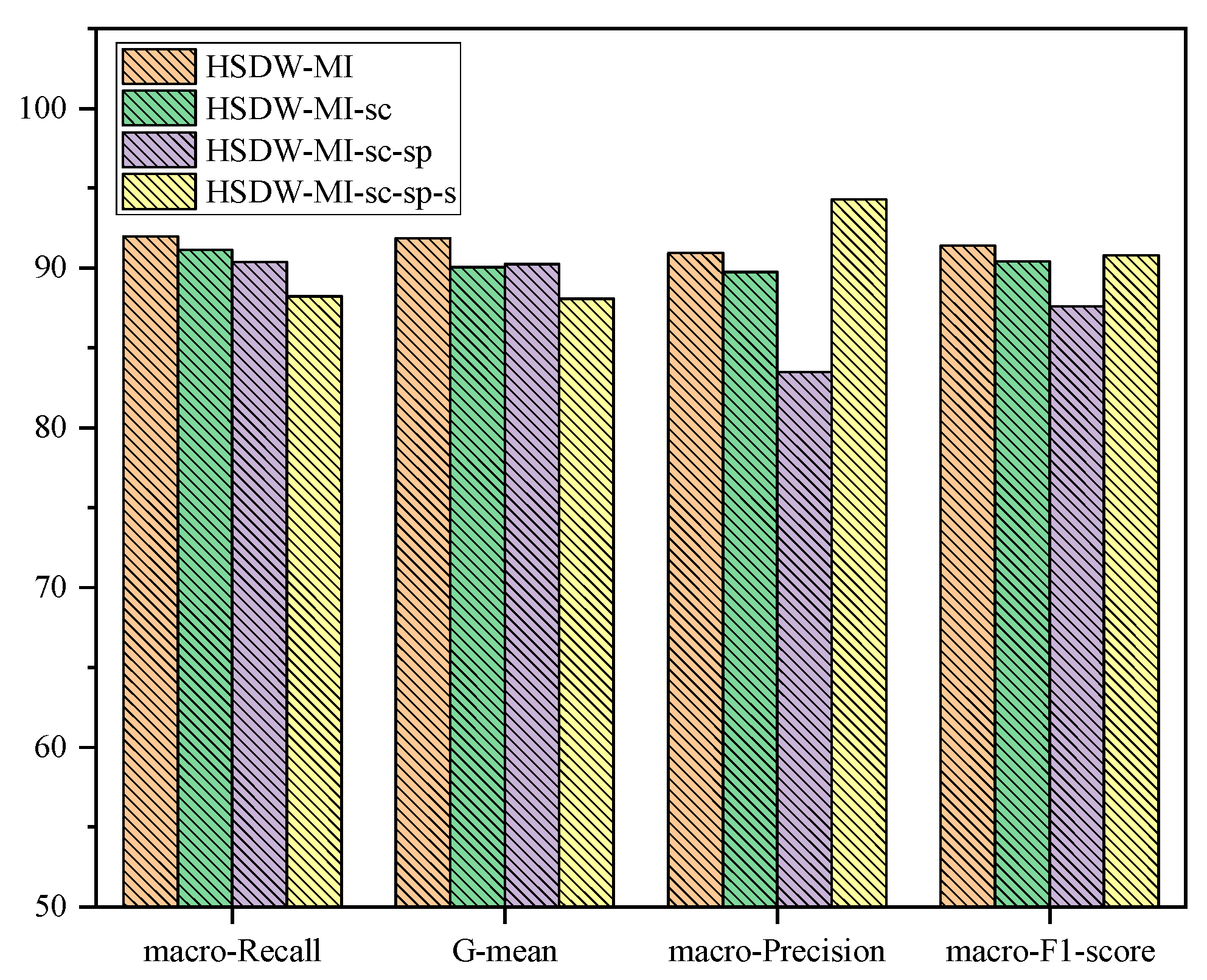
4.3. Ablation Experiments

In this subsection, we analyze the contribution of each component of HSDW-MI for the classification results. First, only the dynamic weighting component is retained in the algorithm, which forms HSDW-MI-sc-sp-s. Then, the sample safety factor sampling component is added based on the previous step, which forms HSDW-MI-sc-sp. Second, the storage pool is added based on the previous step, which forms HSDW-MI-sc. Finally, the spectral clustering is added based on the previous step, which forms HSDW-MI. In order to highlight the effect of the ablation experiment, we use the variable, extremely imbalanced ImbVar_Extreme_SIG data stream with mixed drifts as the experimental data stream, as shown in Figure 3 and Figure 4.

Figure 3 displays the results of each component on macro-Recall, G-mean, macro-Precision, and macro-F1-score metrics. As illustrated in Figure 3, the complete version of the algorithm, HSDW-MI, exhibits the best overall performance on these four metrics, followed by HSDW-MI-sc. In terms of macro-Precision, HSDW-MI-sc-sp-s achieves 94.29, ranking 1st, while HSDW-MI-sc-sp scores 83.49, ranking 4th. This reveals that when sampling is not added, the algorithm focuses more on the majority class samples and exhibits greater accuracy for these samples. However, when sampling is added, the learnability of the majority class samples is impaired. Nevertheless, with the addition of the storage pool and spectral clustering, the algorithm’s macro-Precision value is enhanced, demonstrating an improved ability to classify majority-class samples.

Figure 4 presents the macro-Recall variation curves of each component of the HSDW-MI algorithm on the ImbVar_Extreme_SIG data stream. As shown in Figure 4, the worst performance comes from HSDW-MI-sc-sp-s, which only includes dynamic weighting, as it can only handle concept drift in the data stream and lacks mechanisms to address imbalance and variable data streams. The performance of HSDW-MI-sc-sp improves with the addition of sample safety factor sampling, which better handles imbalance problems. Adding the storage pool further enhances HSDW-MI-sc performance, particularly in phases without concept drift. This is because the selected experimental data streams are extremely imbalanced, and extracting stored instances from the storage pool during the steady stage enables the algorithm to classify minority classes more accurately and effectively cope with variations in class ratio. Finally, the addition of spectral clustering marginally improves the overall performance of the algorithm. However, this addition allows the algorithm’s performance to recover more quickly after concept drift compared to the previous component, as spectral clustering clusters each class, and oversampling or under-sampling based on clusters maintains the original class distribution.

4.4. Algorithm Comparison Experiments

In this subsection, we compare HSDW-MI on 10 synthetic and 3 real data streams with other state-of-the-art algorithms that all of them can learn from multi-class data streams. LB [21], ARF [23], BOLE [25], and OAUE [28] are the online ensemble algorithms, which have concept drift detection mechanism and are mainly used to detect and solve drift problems. MUOB, MOOB [2], and CALMID [24] are ensemble algorithms with imbalance handling mechanism and are able to handle data streams with varying class ratio. The default parameters of all algorithms are set to D = 2000, N = 20, and the ensemble update threshold θ of HSDW-MI is set to 0.5.

Each comparison algorithm is evaluated by using four metrics, including macro-Recall, G-mean, macro-Precision, and macro-F1-score. The results of the algorithm performance are shown in

Table 5. Macro-Recall results (%) of the comparison experiments.

Data Stream		Algorithm
		LB	OAUE	ARF	BOLE	MUOB	MOOB	CALMID	HSDW-MI
Stationary data stream	ImbSta_Stream	96.44(3)	94.45(6)	96.70(2)	94.96(5)	82.52(8)	94.22(7)	96.06(4)	97.21(1)
	ImbSta_Extreme_Stream	93.61(5)	92.14(6)	95.36(2)	91.17(7)	71.74(8)	94.40(4)	94.85(3)	97.13(1)
	ImbSta_SG	90.40(4)	89.07(5)	90.75(3)	86.08(6)	78.13(8)	85.64(7)	91.09(2)	91.99(1)
	ImbSta_Extreme_SG	88.19(3)	83.25(6)	88.13(4)	79.18(7)	66.05(8)	83.67(5)	90.85(2)	92.25(1)
	ImbSta_Extreme_SIG	84.97(4)	80.75(6)	88.54(3)	77.45(7)	63.63(8)	81.82(5)	88.76(2)	92.18(1)
Variable data stream	ImbVar_Stream	76.00(8)	91.75(4)	91.50(5)	92.02(3)	87.57(6)	92.11(2)	86.50(7)	92.64(1)
	ImbVar_Extreme_Stream	90.61(4)	90.84(3)	90.47(5)	90.17(7)	71.06(8)	90.40(6)	91.97(2)	92.59(1)
	ImbVar_SG	91.45(4)	89.26(5)	91.82(3)	87.17(7)	78.01(8)	85.66(6)	92.08(1)	91.91(2)
	ImbVar_Extreme_SG	89.44(4)	85.23(6)	89.52(3)	82.88(7)	70.89(8)	88.90(5)	91.82(2)	92.51(1)
	ImbVar_Extreme_SIG	89.23(4)	68.48(7)	90.23(3)	85.11(6)	61.99(8)	87.97(5)	90.97(2)	92.01(1)
Real Stream	PokerHand	30.81(4)	30.23(5)	27.26(7)	32.32(3)	7.82(8)	33.78(2)	29.50(6)	38.13(1)
	Kddcup 99_10%	35.19(6)	28.29(7)	40.02(3)	44.80(1)	3.12(8)	37.81(5)	40.00(4)	41.09(2)
	Statlog(shuttle)	44.13(7)	45.81(5)	50.12(4)	44.45(6)	17.61(8)	52.41(3)	56.73(2)	78.41(1)

,

Table 6. G-mean results (%) of the comparison experiments.

Data Stream		Algorithm
		LB	OAUE	ARF	BOLE	MUOB	MOOB	CALMID	HSDW-MI
Stationary data stream	ImbSta_Stream	96.37(3)	94.34(6)	96.63(2)	94.72(5)	82.19(8)	94.14(7)	95.96(4)	97.19(1)
	ImbSta_Extreme_Stream	93.23(5)	91.05(6)	95.07(2)	90.12(7)	70.98(8)	94.14(4)	94.35(3)	97.09(1)
	ImbSta_SG	90.13(4)	88.51(5)	90.36(3)	85.38(6)	75.89(8)	83.55(7)	90.76(2)	91.58(1)
	ImbSta_Extreme_SG	86.94(3)	81.39(6)	86.63(4)	76.73(7)	61.40(8)	81.46(5)	87.86(2)	92.21(1)
	ImbSta_Extreme_SIG	83.40(4)	78.72(5)	87.26(3)	74.70(7)	60.91(8)	78.14(6)	89.14(2)	92.17(1)
Variable data stream	ImbVar_Stream	56.86(8)	91.13(5)	91.39(4)	91.72(2)	87.11(6)	91.55(3)	81.57(7)	92.12(1)
	ImbVar_Extreme_Stream	90.23(3)	90.05(7)	90.17(4)	90.12(6)	70.98(8)	90.14(5)	91.58(2)	92.04(1)
	ImbVar_SG	91.19(3)	88.71(5)	91.62(2)	86.51(6)	75.91(8)	84.05(7)	91.96(1)	91.05(4)
	ImbVar_Extreme_SG	88.56(4)	83.76(6)	88.65(3)	80.73(7)	68.26(8)	87.41(5)	91.01(2)	91.95(1)
	ImbVar_Extreme_SIG	87.85(3)	62.15(7)	87.55(4)	82.23(6)	57.97(8)	85.92(5)	90.12(2)	91.87(1)
Real Stream	PokerHand	-	-	-	-	-	-	-	15.16(1)
	Kddcup 99_10%	-	-	-	-	-	-	-	5.47(1)
	Statlog(shuttle)	-	-	-	-	-	-	-	38.80(1)

,

Table 7. Macro-Precision results (%) of the comparison experiments.

Data Stream		Algorithm
		LB	OAUE	ARF	BOLE	MUOB	MOOB	CALMID	HSDW-MI
Stationary data stream	ImbSta_Stream	92.85(3)	88.25(6)	96.21(2)	91.52(5)	70.76(8)	85.82(7)	91.91(4)	96.24(1)
	ImbSta_Extreme_Stream	92.23(4)	88.11(6)	93.45(3)	90.79(5)	58.45(8)	80.14(7)	93.96(2)	94.07(1)
	ImbSta_SG	83.07(5)	84.27(4)	92.69(1)	81.05(6)	65.41(8)	79.19(7)	90.02(3)	92.57(2)
	ImbSta_Extreme_SG	84.62(4)	84.27(5)	86.43(2)	81.84(6)	57.42(8)	76.90(7)	86.89(1)	86.24(3)
	ImbSta_Extreme_SIG	82.30(5)	81.72(6)	84.63(3)	82.75(4)	54.59(8)	74.54(7)	89.77(1)	85.96(2)
Variable data stream	ImbVar_Stream	89.65(4)	89.75(2)	89.67(3)	88.29(6)	80.32(8)	90.45(1)	88.56(5)	88.26(7)
	ImbVar_Extreme_Stream	89.23(4)	88.11(6)	90.47(2)	90.79(1)	58.45(8)	80.14(7)	90.33(3)	88.29(5)
	ImbVar_SG	89.06(4)	84.50(5)	93.15(1)	83.23(6)	65.19(8)	79.26(7)	89.33(3)	92.71(2)
	ImbVar_Extreme_SG	90.10(2)	85.56(6)	90.32(1)	87.68(5)	58.89(8)	81.76(7)	89.82(3)	88.32(4)
	ImbVar_Extreme_SIG	91.30(3)	79.25(7)	91.36(1)	90.71(5)	58.80(8)	86.10(6)	91.35(2)	90.94(4)
Real Stream	PokerHand	44.28(1)	39.87(3)	-	41.69(2)	-	34.73(5)	-	35.03(4)
	Kddcup 99_10%	-	-	-	-	-	-	-	56.91(1)
	Statlog(shuttle)	-	-	13.48(3)	5.93(4)	-	40.44(2)	6.86(5)	75.05(1)

and

Table 8. Macro-F1-score results (%) of the comparison experiments.

Data Stream		Algorithm
		LB	OAUE	ARF	BOLE	MUOB	MOOB	CALMID	HSDW-MI
Stationary data stream	ImbSta_Stream	94.61(3)	91.24(6)	96.45(2)	93.21(5)	76.19(8)	89.82(7)	93.94(4)	96.72(1)
	ImbSta_Extreme_Stream	92.91(4)	90.08(6)	94.40(2)	90.98(5)	64.42(8)	86.69(7)	94.40(2)	95.58(1)
	ImbSta_SG	86.58(5)	86.60(4)	91.71(2)	83.49(6)	71.21(8)	82.29(7)	90.55(3)	92.28(1)
	ImbSta_Extreme_SG	86.37(4)	83.76(5)	87.27(3)	80.49(6)	61.43(8)	80.14(7)	88.83(2)	89.14(1)
	ImbSta_Extreme_SIG	83.61(4)	81.23(5)	86.54(3)	80.01(6)	58.76(8)	78.01(7)	89.26(1)	88.96(2)
Variable data stream	ImbVar_Stream	82.26(8)	90.74(2)	90.58(3)	90.12(5)	83.79(7)	91.27(1)	87.52(6)	90.40(4)
	ImbVar_Extreme_Stream	89.91(5)	89.45(6)	90.47(3)	90.48(2)	64.14(8)	84.96(7)	91.14(1)	90.39(4)
	ImbVar_SG	90.24(4)	86.81(5)	92.48(1)	85.15(6)	71.03(8)	82.34(7)	90.68(3)	92.31(2)
	ImbVar_Extreme_SG	89.77(4)	85.39(5)	89.92(3)	85.21(6)	64.34(8)	85.18(7)	90.81(1)	90.37(2)
	ImbVar_Extreme_SIG	90.25(4)	73.47(7)	90.79(3)	87.82(5)	60.35(8)	87.02(6)	91.16(2)	91.47(1)
Real Stream	PokerHand	36.34(3)	34.39(4)	-	36.41(2)	-	34.25(5)	-	36.51(1)
	Kddcup 99_10%	-	-	-	-	-	-	-	47.72(1)
	Statlog(shuttle)	-	-	21.25(3)	10.46(5)	-	45.65(2)	12.24(4)	76.69(1)

. The results of the algorithm with the best performance are highlighted in bold.

As shown in Table 5 and Table 6, HSDW-MI achieves the best macro-Recall and G-mean values for all synthetic and real data streams, ranking first, followed by the CALMID and ARF algorithms. For stationary, extremely imbalanced streams, HSDW-MI outperforms all other algorithms, with an average of 2.19% higher macro-Recall values and 3.13% higher G-mean values. In variable streams, HSDW-MI performs best overall, particularly excelling on ImbVar_Extreme_SG and ImbVar_Extreme_SIG with mixed drift, averaging 0.87% higher macro-Recall, and 1.35% higher G-mean values. The second-ranked algorithm is the state-of-the-art CALMID, which effectively handles differences between majority and minority classes using the asymmetric margin threshold matrix and uncertainty strategy. CALMID also proposed a composite sample weight formula that assigns higher training weights to newly arrived and minority samples, accommodating data stream imbalance and concept drift. The ARF algorithm ranks third, even though it lacks a mechanism to handle class imbalance. However, ARF requires significant time to maintain the detector and training tree. LB, OAUE, and BOLE algorithms perform poorly on extremely imbalanced data streams but achieve better results on other streams. The MOOB algorithm, with resampling and time decay techniques, performs better only on data streams without concept drift, as it lacks a mechanism to handle such drift. MUOB cannot adapt to complex data streams because under-sampling results in substantial sample information loss. Overall, HSDW-MI achieves the best macro-Recall and G-mean values, ranking first and demonstrating its effectiveness in identifying minority class instances, especially in extremely imbalanced data streams.

As shown in Table 7 and Table 8, HSDW-MI attains better macro-Precision and macro-F1-score values only on stationary data streams, while it is slightly outperformed by the ARF and CALMID on variable data streams. This is because both macro-Precision and macro-F1-score metrics focus more on majority class classification. In HSDW-MI, the class ratio-based sampling approach calculates too many majority class samples requiring under-sampling, which somewhat impairs the learnability of majority class samples.

For real data streams, HSDW-MI achieves the best results for macro-Recall and G-mean values. On the PokerHand dataset, LB ranks first in macro-Precision and macro-F1-score, while HSDW-MI has lower performance than other algorithms. It is worth noting that most algorithms display 0 in G-mean, macro-Precision, and macro-F1-score. It is due to the fact that the real data stream contains a large number of classes, and the number of minority class instances may be single-digit, resulting in 0 values for macro-Precision, macro-F1-score, and G-mean. This also demonstrates that HSDW-MI can handle the severe lack of minority class samples and adapt to extremely imbalanced data streams.

To better illustrate each algorithm’s performance on data streams, we present the run results of all algorithms on ImbSta_Extreme_SG, ImbSta_Extreme_SIG, ImbVar_Extreme_SG, and ImbVar_Extreme_SIG data streams in the form of line graphs, as shown in Figure 5 and Figure 6.

As shown in Figure 5a,b, the best performance in the stationary data streams is the HSDW-MI algorithm, followed by the CALMID and ARF algorithms. The CALMID and ARF algorithms also show better performance when no concept drift occurs, even close to that of HSDW-MI. In the stage after the first drift in Figure 5a, the HSDW-MI algorithm’s performance is slightly lower than the other algorithms, but HSDW-MI is able to recover from the drift faster and its overall performance is still the best. As shown in Figure 6a,b, the HSDW-MI algorithm still shows excellent performance in the stage without concept drift in the variable data streams, followed by the CALMID, ARF, LB, and MOOB algorithms. In conclusion, the HSDW-MI algorithm performs best when no concept drift occurs, demonstrating the ability of the HSDW-MI algorithm to handle data streams with extreme imbalance and variable class ratio and perform best. The macro-Recall values of all algorithms drop sharply when drift occurs, in which CALMID and LB algorithms are better able to adapt to concept drift and have better performance at the drift point, while HSDW-MI algorithm is able to recover from the drift faster. That is because the dynamic weighting strategy of the HSDW-MI algorithm is able to remove unqualified classifiers in time, and, thus, the HSDW-MI algorithm is able to recover performance faster after the drift occurring.

5. Summary

To address the problems of multiclass imbalance and concept drift in data streams, this paper proposed a multi-class imbalanced data stream classification algorithm based on hybrid sampling with dynamic weighting (HSDW-MI). HSDW-MI processes data streams in two phases. In the hybrid sampling phase, adaptive spectral clustering is used to maintain the original data distribution after clustering and sampling. By calculating the safety level of each sample using the sample safety factor, the classifier’s ability to identify both minority and majority classes is effectively improved. To handle extremely imbalanced and variable data streams, a sample storage pool is created to store samples with high safety factor during the training process. Samples are extracted from the pool and added to the data stream when the number of minority class samples is insufficient. In the dynamic weighting phase, a dynamic weighting method based on G-mean values is proposed, with G-mean values serving as the weights of the base classifier. The ensemble is dynamically updated during data stream processing by adding new base classifiers and timely removing old, unqualified ones, which allows the algorithm to adapt to concept drift. Experiments verify that the proposed HSDW-MI exhibits superior classification capabilities and more Stable performance than other algorithms.

Despite its merits, the algorithm still has some limitations due to the complexity of multi-class imbalanced data streams. Although HSDW-MI can recover quickly after a concept drift occurrence, its performance degrades more at the concept drift point compared to other algorithms. Additionally, calculating the sample safety factor is time-consuming. Future research will incorporate a drift detector into the algorithm, enabling it to address concept drift upon detection, and refine the sample safety factor calculation formula to reduce time complexity.

References

1. Ancy, S.; Paulraj, D. Handling imbalanced data with concept drift by applying dynamic sampling and ensemble classification model. Comput. Commun. 2020, 153, 553–560. [Google Scholar] [CrossRef]
2. Wang, S.; Minku, L.L.; Yao, X. Dealing with Multiple Classes in Online Class Imbalance Learning. In Proceedings of the 25th International Joint Conference on Artificial Intelligence, New York, NY, USA, 9–15 July 2016; pp. 2118–2124. [Google Scholar]
3. Kaddoura, S.; Arid, A.E.; Moukhtar, M. Evaluation of Supervised Machine Learning Algorithms for Multi-Class Intrusion Detection Systems. In Proceedings of the Future Technologies Conference (FTC) 2021; Springer: Berlin/Heidelberg, Germany, 2022; Volume 3, pp. 1–16. [Google Scholar]
4. Bin Sulaiman, R.; Schetinin, V.; Sant, P. Review of Machine Learning Approach on Credit Card Fraud Detection. Hum. Cent. Intell. Syst. 2022, 2, 55–68. [Google Scholar] [CrossRef]
5. Ahsan, M.M.; Luna, S.A.; Siddique, Z. Machine-learning-based disease diagnosis: A comprehensive review. Healthcare 2022, 10, 541. [Google Scholar] [CrossRef]
6. Lu, J.; Liu, A.; Dong, F.; Gu, F.; Gama, J.; Zhang, G. Learning under concept drift: A review. IEEE Trans. Knowl. Data Eng. 2018, 31, 2346–2363. [Google Scholar] [CrossRef]
7. Zhang, X.; Han, M.; Wu, H.; Li, M.; Chen, Z. An overview of complex data stream ensemble classification. J. Intell. Fuzzy Syst. 2021, 41, 3667–3695. [Google Scholar] [CrossRef]
8. Mirza, B.; Lin, Z. Meta-cognitive online sequential extreme learning machine for imbalanced and concept-drifting data classification. Neural Netw. 2016, 80, 79–94. [Google Scholar] [CrossRef] [PubMed]
9. Ferreira, L.E.B.; Gomes, H.M.; Bifet, A.; Oliveira, L.S. Adaptive random forests with resampling for imbalanced data streams. In Proceedings of the International Joint Conference on Neural Networks (IJCNN), Budapest, Hungary, 14–19 July 2019; pp. 1–6. [Google Scholar]
10. Abdi, L.; Hashemi, S. To combat multi-class imbalanced problems by means of over-sampling techniques. IEEE Trans. Knowl. Data Eng. 2015, 28, 238–251. [Google Scholar] [CrossRef]
11. Zhu, T.; Lin, Y.; Liu, Y. Synthetic minority oversampling technique for multiclass imbalance problems. Pattern Recognit. J. Pattern Recognit. Soc. 2017, 72, 327–340. [Google Scholar] [CrossRef]
12. Arafat, M.Y.; Hoque, S.; Farid, D.M. Cluster-based under-sampling with random forest for multi-class imbalanced classification. In Proceedings of the 11th International Conference on Software, Knowledge, Information Management and Applications (SKIMA), Malabe, Sri Lanka, 6–8 December 2017; pp. 1–6. [Google Scholar]
13. Díez-Pastor, J.F.; Rodríguez, J.J.; Garcia-Osorio, C.; Kuncheva, L.I. Random balance: Ensembles of variable priors classifiers for imbalanced data. Knowl.-Based Syst. 2015, 85, 96–111. [Google Scholar] [CrossRef]
14. Rodríguez, J.J.; Diez-Pastor, J.F.; Arnaiz-Gonzalez, A.; Kuncheva, L.I. Random balance ensembles for multiclass imbalance learning. Knowl.-Based Syst. 2020, 193, 105434. [Google Scholar] [CrossRef]
15. Hartono, H.; Risyani, Y.; Ongko, E.; Abdullah, D. HAR-MI method for multi-class imbalanced datasets. Telecommun. Comput. Electron. Control 2020, 18, 822–829. [Google Scholar] [CrossRef]
16. Jadwal, P.K.; Jain, S.; Pathak, S.; Agarwal, B. Improved resampling algorithm through a modified oversampling approach based on spectral clustering and SMOTE. Microsyst. Technol. 2022, 28, 2669–2677. [Google Scholar] [CrossRef]
17. Sainin, M.S.; Alfred, R.; Adnan, F.; Ahmad, F. Combining sampling and ensemble classifier for multiclass imbalance data learning. In Proceedings of the International Conference on Computational Science and Technology, Labuan, Malaysia, 28–29 August 2021; Springer: Singapore, 2017; pp. 262–272. [Google Scholar]
18. Vafaie, P.; Viktor, H.; Michalowski, W. Multi-class imbalanced semi-supervised learning from streams through online ensembles. In Proceedings of the International Conference on Data Mining Workshops, Sorrento, Italy, 17–20 November 2020; pp. 867–874. [Google Scholar]
19. Czarnowski, I. Weighted Ensemble with one-class Classification and Over-sampling and Instance selection (WECOI): An approach for learning from imbalanced data streams. J. Comput. Sci. 2022, 61, 101614. [Google Scholar] [CrossRef]
20. Han, M.; Zhang, X.; Chen, Z.; Wu, H.; Li, M. Dynamic ensemble selection classification algorithm based on window over imbalanced drift data stream. Knowl. Inf. Syst. 2022, 65, 1105–1128. [Google Scholar] [CrossRef]
21. Bifet, A.; Holmes, G.; Pfahringer, B. Leveraging bagging for evolving data streams. In Machine Learning and Knowledge Discovery in Databases: European Conference, ECML PKDD 2010, Barcelona, Spain, 20–24 September 2010, Proceedings, Part I 21; Springer: Berlin/Heidelberg, Germany, 2010; pp. 135–150. [Google Scholar]
22. Bifet, A.; Gavalda, R. Learning from time-changing data with adaptive windowing. In Proceedings of the 7th SIAM International Conference on Data Mining, Minneapolis, MN, USA, 26–28 April 2007; pp. 443–448. [Google Scholar]
23. Gomes, H.M.; Bifet, A.; Read, J.; Barddal, J.P.; Enembreck, F.; Pfharinger, B.; Holmes, G.; Abdessalem, T. Adaptive random forests for evolving data stream classification. Mach. Learn. 2017, 106, 1469–1495. [Google Scholar] [CrossRef]
24. Liu, W.; Zhang, H.; Ding, Z.; Liu, Q.; Zhu, C. A comprehensive active learning method for multiclass imbalanced data streams with concept drift. Knowl.-Based Syst. 2021, 215, 106778. [Google Scholar] [CrossRef]
25. De Barros, R.S.M.; de Carvalho Santos, S.G.T.; Júnior, P.M.G. A boosting-like online learning ensemble. In Proceedings of the 2016 International Joint Conference on Neural Networks (IJCNN), Vancouver, BC, Canada, 24–29 July 2016; pp. 1871–1878. [Google Scholar]
26. Iwashita, A.S.; Papa, J.P. An overview on concept drift learning. IEEE Access 2018, 7, 1532–1547. [Google Scholar] [CrossRef]
27. Han, M.; Chen, Z.; Li, M.; Wu, H.; Zhang, X. A survey of active and passive concept drift handling methods. Comput. Intell. 2022, 38, 1492–1535. [Google Scholar] [CrossRef]
28. Brzezinski, D.; Stefanowski, J. Combining chunk-based and online methods in learning ensembles from concept drifting data streams. Inf. Sci. 2014, 265, 50–67. [Google Scholar] [CrossRef]
29. Ertunç, E.; Karkınlı, A.E.; Bozdağ, A. A clustering-based approach to land valuation in land consolidation projects. Land Use Policy 2021, 111, 105739. [Google Scholar] [CrossRef]
30. Janicka, M.; Lango, M.; Stefanowski, J. Using information on class interrelations to improve classification of multiclass imbalanced data: A new resampling algorithm. Int. J. Appl. Math. Comput. Sci. 2019, 29, 769–781. [Google Scholar] [CrossRef]
31. Lango, M.; Stefanowski, J. Multi-class and feature selection extensions of roughly balanced bagging for imbalanced data. J. Intell. Inf. Syst. 2018, 50, 97–127. [Google Scholar] [CrossRef]
32. Mahadevan, A.; Arock, M. A class imbalance-aware review rating prediction using hybrid sampling and ensemble learning. Multimed. Tools Appl. 2021, 80, 6911–6938. [Google Scholar] [CrossRef]
33. Bifet, A.; Holmes, G.; Pfahringer, B.; Kranen, P.; Kremer, H.; Jansen, T.; Seidl, T. Moa: Massive online analysis, a framework for stream classification and clustering. In Proceedings of the First Workshop on Applications of Pattern Analysis, Windsor, UK, 1–3 September 2010; pp. 44–50. [Google Scholar]
Figure 1. Concept drift types.
Applsci 13 05924 g001
Figure 2. The framework of HSDW-MI algorithm.
Applsci 13 05924 g002
Figure 3. Results of ablation experiment on the ImbVar_Extreme_SIG stream.
Applsci 13 05924 g003
Figure 4. Macro-Recall of ablation experiment on the ImbVar_Extreme_SIG stream.
Applsci 13 05924 g004
Figure 5. Comparison algorithm of macro-Recall on the stationary stream. (a) ImbSta_Extreme_SG stream; (b) ImbSta_Extreme_SIG.
Applsci 13 05924 g005
Figure 6. Comparison algorithm of macro-Recall on the variable stream. (a) ImbVar_Extreme_SG stream; (b) ImbVar_Extreme_SIG.
Applsci 13 05924 g006